Contact Geometry of second order I - Dept. Math, Hokkaido Univ ...

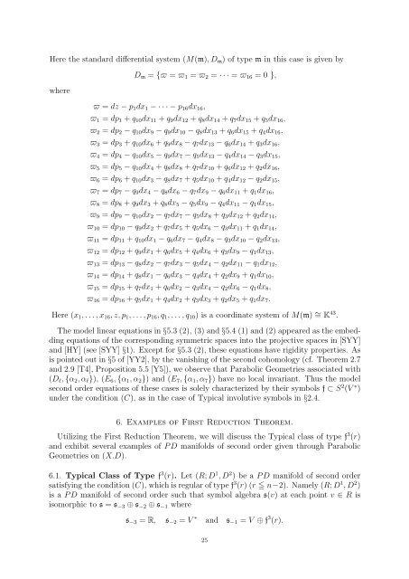
Here the standard differential system (M(m), Dm) of type m in this case is given by
where
Dm = {ϖ = ϖ1 = ϖ2 = · · · = ϖ16 = 0 },
ϖ = dz − p1dx1 − · · · − p16dx16,
ϖ1 = dp1 + q10dx11 + q9dx12 + q8dx14 + q7dx15 + q5dx16,
ϖ2 = dp2 − q10dx9 − q9dx10 − q8dx13 + q6dx15 + q4dx16,
ϖ3 = dp3 + q10dx6 + q9dx8 − q7dx13 − q6dx14 + q3dx16,
ϖ4 = dp4 − q10dx5 − q9dx7 − q5dx13 − q4dx14 − q3dx15,
ϖ5 = dp5 − q10dx4 + q8dx8 + q7dx10 + q6dx12 + q2dx16,
ϖ6 = dp6 + q10dx3 − q8dx7 + q5dx10 + q4dx12 − q2dx15,
ϖ7 = dp7 − q9dx4 − q8dx6 − q7dx9 − q6dx11 + q1dx16,
ϖ8 = dp8 + q9dx3 + q8dx5 − q5dx9 − q4dx11 − q1dx15,
ϖ9 = dp9 − q10dx2 − q7dx7 − q5dx8 + q3dx12 + q2dx14,
ϖ10 = dp10 − q9dx2 + q7dx5 + q5dx6 − q3dx11 + q1dx14,
ϖ11 = dp11 + q10dx1 − q6dx7 − q4dx8 − q3dx10 − q2dx13,
ϖ12 = dp12 + q9dx1 + q6dx5 + q4dx6 + q3dx9 − q1dx13,
ϖ13 = dp13 − q8dx2 − q7dx3 − q5dx4 − q2dx11 − q1dx12,
ϖ14 = dp14 + q8dx1 − q6dx3 − q4dx4 + q2dx9 + q1dx10,
ϖ15 = dp15 + q7dx1 + q6dx2 − q3dx4 − q2dx6 − q1dx8,
ϖ16 = dp16 + q5dx1 + q4dx2 + q3dx3 + q2dx5 + q1dx7.
Here (x1, . . . , x16, z, p1, . . . , p16, q1, . . . , q10) is a coordinate system of M(m) ∼ = K 43 .
The model linear equations in §5.3 (2), (3) and §5.4 (1) and (2) appeared as the embedding
equations of the corresponding symmetric spaces into the projective spaces in [SYY]
and [HY] (see [SYY] §1). Except for §5.3 (2), these equations have rigidity properties. As
is pointed out in §5 of [YY2], by the vanishing of the second cohomology (cf. Theorem 2.7
and 2.9 [T4], Proposition 5.5 [Y5]), we observe that Parabolic Geometries associated with
(Dℓ, {α2, αℓ}), (E6, {α1, α2}) and (E7, {α1, α7}) have no local invariant. Thus the model
second order equations of these cases is solely characterized by their symbols f ⊂ S 2 (V ∗ )
under the condition (C), as in the case of Typical involutive symbols in §2.4.
6. Examples of First Reduction Theorem.
Utilizing the First Reduction Theorem, we will discuss the Typical class of type f 3 (r)
and exhibit several examples of P D manifolds of second order given through Parabolic
Geometries on (X.D).
6.1. Typical Class of Type f 3 (r). Let (R; D 1 , D 2 ) be a P D manifold of second order
satisfying the condition (C), which is regular of type f 3 (r) (r ≦ n−2). Namely (R; D 1 , D 2 )
is a P D manifold of second order such that symbol algebra s(v) at each point v ∈ R is
isomorphic to s = s−3 ⊕ s−2 ⊕ s−1 where
s−3 = R, s−2 = V ∗
25
and s−1 = V ⊕ f 3 (r).