Contact Geometry of second order I - Dept. Math, Hokkaido Univ ...

More documents

Recommendations

Info

$2 - Dept. Math, Hokkaido Univ. EPrints Server$

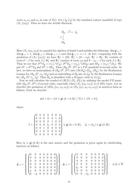
oots α1,α3 and α4 in case of D4): Let (Jg, Cg) be the standard contact manifold of type (Xℓ, {αθ}). Then we have the double fibration; πg Rg ⏐ Mg πc −−−→ Jg Here (Xℓ, {αθ, αG}) is a graded Lie algebra of depth 5 and satisfies the following: dim ˇg−5 = dim ˇg−4 = 1, dim ˇg−3 = dim ˇg−2 = s and dim ˇg−1 = s + 1. In fact, comparing with the gradation of (Xℓ, {αG}), we have ˇ Φ + 5 = {θ}, ˇ Φ + 4 = {θ − αθ}, ˇ Φ + 3 = Φ + 2 , ˇ Φ + 2 consists of roots θ − β for each β ∈ ˇ Φ + 3 and ˇ Φ + 1 consists of roots αθ and θ − αθ − β for each β ∈ ˇ Φ + 3 . Thus we see that ∂ (3) Eg = (πc) −1 ∗ (Cg), ∂ (2) Eg = (πg) −1 ∗ (∂Dg) and ∂Eg = (πg) −1 ∗ (Dg). We put D1 = ∂ (3) Eg and D2 = ∂Eg. Then (Rg; D1 , D2 ) is a P D manifold of second order. In fact, we have an isomorphism of (Rg; D1 , D2 ) onto (R(Mg); D1 Mg , D2 ) by the Realization Mg Lemma for (Rg, D1 , πg, Mg) and an embedding of Rg into L(Jg) by the Realization Lemma for (Rg, D2 , πc, Jg). Thus Rg is identified with a R-space orbit in L(Jg). ) by utilizing the model P D mani- Now we will calculate the symbol of (R(X); D1 X , D2 X fold (Rg; D1 , D2 ) of second order, especially when (Xℓ, {αθ, αG}) is of BDℓ types. Let us describe the gradation of (BDℓ, {α1, α2, α3}) or (D4, {α1, α2, α3, α4}) in matrices form as follows: First we describe where o(k + 6) = {X ∈ gl (k + 6, K) | t XJ + JX = 0 }, ⎛ 0 0 0 0 0 0 ⎞ 1 ⎜0 ⎜ ⎜0 ⎜ J = ⎜0 ⎜ ⎜0 ⎝ 0 0 0 0 0 1 0 0 0 1 0 0 0 Ik 0 0 0 1 0 0 0 1 0 0 0 0 0 ⎟ 0 ⎟ 0⎟ ∈ gl (k + 6, K), ⎟ 0⎟ 0 ⎠ Ik = (δij) ∈ gl (k, K). 1 0 0 0 0 0 0 Here Ik ∈ gl (k, K) is the unit matrix and the gradation is given again by subdividing matrices as follows; ˇg−5 = ⎧ ⎛ ⎞⎫ ⎧ ⎛ ⎞⎫ 0 0 0 0 0 0 0 0 0 0 0 0 0 0 ⎜0 0 0 0 0 0 0⎟ ⎜ 0 0 0 0 0 0 0⎟ ⎪⎨ ⎜ ⎟ ⎜0 0 0 0 0 0 0⎟⎪⎬ ⎪⎨ ⎜ ⎟ ⎜ 0 0 0 0 0 0 0⎟⎪⎬ ⎜ ⎟ ⎜ ⎟ ⎜0 0 0 0 0 0 0⎟ , ˇg−4 = ⎜ 0 0 0 0 0 0 0⎟ , y, ξ0 ∈ K ⎜ ⎟ ⎜ ⎟ ⎜0 0 0 0 0 0 0⎟ ⎜ξ0 0 0 0 0 0 0⎟ ⎝ ⎪⎩ y 0 0 0 0 0 0 ⎠ ⎝ ⎪⎭ ⎪⎩ 0 0 0 0 0 0 0 ⎠ ⎪⎭ 0 −y 0 0 0 0 0 0 0 −ξ0 0 0 0 0 28
⎧ ⎛ 0 ⎜0 ⎪⎨ ⎜ ⎜0 ⎜ ⎜ξ ⎜ ⎜0 ⎝ ⎪⎩ 0 0 0 0 0 0 ξ1 0 0 0 0 0 0 0 −ξ1 0 0 0 0 0 0 0 − 0 0 0 0 0 0 0 0 0 0 0 0 0 0 0 0 0 0 tξ 0 0 ⎞ ⎟ ⎟ ⎟ ⎟ ⎟ ξ ∈ K ⎟ ⎟ ⎠ 0 k ⎫ ⎪⎬ , ξ1 ∈ K , ⎪⎭ ⎧ ⎛ 0 ⎜ 0 ⎪⎨ ⎜ ⎜x1 ⎜ 0 ⎜ 0 ⎝ ⎪⎩ 0 0 0 0 x 0 0 0 0 0 0 0 0 0 0 0 0 0 − 0 0 0 0 0 0 0 0 0 0 0 0 0 0 0 t 0 0 0 x 0 0 −x1 0 0 ⎞ ⎟ ⎟ ⎟ ⎟ ⎟ = ˆx + ˆx1 x ∈ K ⎟ ⎟ 0 ⎠ 0 k ⎫ ⎪⎬ , x1 ∈ K , ⎪⎭ ⎧ ⎛ 0 ⎜a1 ⎪⎨ ⎜ 0 ⎜ 0 ⎜ 0 ⎝ ⎪⎩ 0 0 x0 0 0 0 0 0 a 0 0 0 0 0 − 0 0 0 0 0 0 0 0 0 0 0 0 t 0 0 0 0 0 0 a 0 0 0 −x0 0 0 0 −a1 ⎞ ⎟ ⎟ ⎟ ⎟ ⎟ = ˆx0 + â1 + â ⎟ 0⎟ 0 ⎠ 0 x0, a1 ∈ K, a ∈ K k ⎫ ⎪⎬ , ⎪⎭ ˇg0 ⎧ ⎛ b ⎜0 ⎪⎨ ⎜ ⎜0 ⎜ = ⎜0 ⎜ ⎜0 ⎝ ⎪⎩ 0 0 0 c 0 0 0 0 0 0 0 e 0 0 0 0 0 0 0 B 0 0 0 0 0 0 0 −e 0 0 0 0 0 0 0 −c 0 ⎞ ⎫ 0 0 ⎟ ⎟ 0 ⎟ ⎪⎬ ⎟ 0 ⎟ b, c, e ∈ K, B ∈ o(k) ⎟ 0 ⎟ 0 ⎠ ⎪⎭ −b ˇg−3 = ˇg−2 = ˇg−1 = ˇgℓ = { t X | X ∈ g−ℓ }, (ℓ = 1, 2, 3, 4, 5), Then, for X = ˆx + ˆx1 + ˆx0 and A = â + â1 , we calculate Thus we obtain [[A, X], X] = (2x1 t ax − a1 t xx) ∈ ˇg−5 f = 〈{2e ∗ 1 ⊚ e ∗ 2, . . . , 2e ∗ 1 ⊚ e ∗ k+1, e ∗ 2 ⊚ e ∗ 2 + · · · + e ∗ k+1 ⊚ e ∗ k+1〉 ⊂ S 2 (E ⊥ ), where {e0, e1, . . . , ek+1} is a basis of V and E = 〈{e0}〉 is the Cauchy characteristic direction. In case k = 1, f = 〈{2e∗ 1 ⊚ e∗ 2, e∗ 2 ⊚ e∗ 2}〉 is an involutive subspace of S2 (E⊥ ). Hence (Rg; D1 , D2 ) is involutive when g = ⊕ p∈Z gp is of type (B3, {α1, α2, α3}). In case k > 1, we have f ⊥ = 〈{e1 ⊚ e1, ei ⊚ ej(2 ≦ i < j ≦ k + 1), e2 ⊚ e2 − ek+1 ⊚ ek+1, . . . , ek ⊚ ek − ek+1 ⊚ ek+1}〉 ⊂ S 2 (W ), where W = 〈{e1, . . . , ek+1}〉. Then we see that (f (1) ) ⊥ contains every ei ⊚ ei ⊚ ei for i = 1, . . . , k + 1, which implies f is of finite type. We can also check that exceptional cases other than G2 are of finite type by utilizing R-space orbit (Rg; D 1 , D 2 ), whereas 29
Page 1 and 2: CONTACT GEOMETRY OF SECOND ORDER I
Page 3 and 4: (2) There exists a coframe { ϖ, ω
Page 5 and 6: Let πp be the projection of D p (x
Page 7 and 8: 3. Symbols of Second Order Equation
Page 9 and 10: The third case occurs when we class
Page 11 and 12: Proof. Fist we observe that S 2 (V
Page 13 and 14: Here (R.2) follows from dϖ ≡ 0 (
Page 15 and 16: iff w⌋f = 0 for all f ∈ f(v). T
Page 17 and 18: for each v ∈ P (X) and x = ν(v),
Page 19 and 20: Next we consider the algebraic prol
Page 21 and 22: For the real version of this theore
Page 23 and 24: where the gradation is given by sub
Page 25 and 26: Here the standard differential syst
Page 27: where ˆϖ = dz − n∑ α=r+1 pα
Page 31 and 32: Hence, from ∑ℓ−2 α,β=1 aα
Page 33 and 34: Let (X, D) be a regular differentia
Page 35 and 36: − p13dx17 − p14dx18 − p15dx19
Page 37 and 38: ∂ 2 z ∂x1∂x16 ∂ 2 z ∂x2
Page 39: References [Bai] T.N.Baily, Parabol

Contact Geometry of second order I - Dept. Math, Hokkaido Univ ...

You also want an ePaper? Increase the reach of your titles

Delete template?

Save as template?