Application Note #AN-00MX-001 - Responsive Environments Group

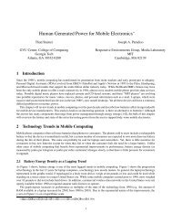
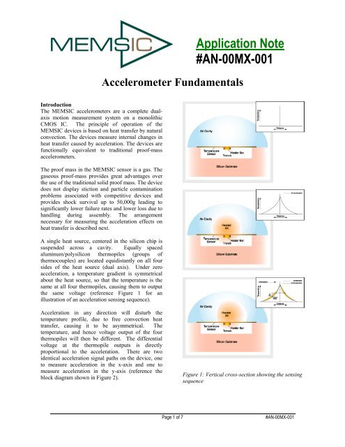
Introduction
The MEMSIC accelerometers are a complete dualaxis
motion measurement system on a monolithic
CMOS IC. The principle of operation of the
MEMSIC devices is based on heat transfer by natural
convection. The devices measure internal changes in
heat transfer caused by acceleration. The devices are
functionally equivalent to traditional proof-mass
accelerometers.
The proof mass in the MEMSIC sensor is a gas. The
gaseous proof-mass provides great advantages over
the use of the traditional solid proof mass. The device
does not display stiction and particle contamination
problems associated with competitive devices and
provides shock survival up to 50,000g leading to
significantly lower failure rates and lower loss due to
handling during assembly. The arrangement
necessary for measuring the acceleration effects on
heat transfer is described next.
A single heat source, centered in the silicon chip is
suspended across a cavity. Equally spaced
aluminum/polysilicon thermopiles (groups of
thermocouples) are located equidistantly on all four
sides of the heat source (dual axis). Under zero
acceleration, a temperature gradient is symmetrical
about the heat source, so that the temperature is the
same at all four thermopiles, causing them to output
the same voltage (reference Figure 1 for an
illustration of an acceleration sensing sequence).
Acceleration in any direction will disturb the
temperature profile, due to free convection heat
transfer, causing it to be asymmetrical. The
temperature, and hence voltage output of the four
thermopiles will then be different. The differential
voltage at the thermopile outputs is directly
proportional to the acceleration. There are two
identical acceleration signal paths on the device, one
to measure acceleration in the x-axis and one to
measure acceleration in the y-axis (reference the
block diagram shown in Figure 2).
Application Note
#AN-00MX-001
Accelerometer Fundamentals
Figure 1: Vertical cross-section showing the sensing
sequence
Page 1 of 7 #AN-00MX-001

Acceleration Measurement Range and
Accelerometer Outputs
The MEMSIC devices are capable of measuring
accelerations with a full-scale range from below ±
1.0g to above ±100g. The devices can measure both
dynamic acceleration (e.g. vibration) and static
acceleration (e.g. gravity).
The devices can provide analog or digital output
voltages. Analog output voltages are available in
absolute and ratiometric mode. The absolute output
voltage is independent of the supply voltage, while
the ratiometric output voltage is proportional to the
supply voltage. The digital outputs are signals with
duty cycles (ratio of pulse width to period) that vary
with acceleration.
The resolution, or the smallest detectable increment
in acceleration is defined by the signal noise. For the
MEMSIC accelerometers the typical noise floor is
below 1mg/ Hz , allowing sub milli-g signals to be
measured at very low frequencies.
The frequency response, or the capability to measure
fast changes in acceleration is defined by design. For
these devices the -3dB rolloff occurs at above 30 Hz
but is expandable to >160 Hz (reference Application
Note AN-00MX-003).
Sck
(optional)
CLK
Heater
Control
2-AXIS
SENSOR
Internal
Oscillator
X axis
Y axis
Continous
Self Test
Factory Adjust
Offset & Gain
Temperature
Sensor
Voltage
Reference
Low Pass
Filter
Low Pass
Filter
Vdd Gnd Vda
Figure 2: Typical Block Diagram
Tout
Vref
Aout X
Aout Y
Application Note
#AN-00MX-001
Packaging and Operating Range
The accelerometers are available in a low-profile
LCC surface mount package (2.00 mm height). They
are hermetically sealed and are operational over a
-40°C to +105°C temperature range.
1
2
3
Y +g
Page 2 of 7 #AN-00MX-001
8
MEMSIC
4
Top View
7
6
5
X +g
Pin Description: LCC-8 Package
Pin Name Description
1 TOUT Temperature (Analog Voltage)
2 AOUTY Y-Axis Acceleration Signal
3 Gnd Ground
4 VDA Analog Supply Voltage
5 AOUTX X-Axis Acceleration Signal
6 Vref 2.5V Reference
7 Sck Optional External Clock
8 VDD Digital Supply Voltage
Figure 3: Sample package and pin-outs

Pin Descriptions
VDD – This is the supply input for the digital circuits
and the sensor heater. The DC voltage should be
between 2.70 and 5. 5 volts.
VDA – This is the power supply input for the analog
amplifiers.
Gnd – This is the ground pin.
AOUTX – This pin is the output of the x-axis
acceleration sensor. The user should ensure the load
impedance is sufficiently high as to not source/sink
>100µA typical. While the sensitivity of this axis has
been programmed at the factory to be the same as the
sensitivity for the y-axis, the device can be
programmed for non-equal sensitivities on the x- and
y-axes.
AOUTY – This pin is the output of the y-axis
acceleration sensor. The user should ensure the load
impedance is sufficiently high as to not source/sink
>100µA typical. While the sensitivity of this axis has
been programmed at the factory to be the same as the
sensitivity for the x-axis, the device can be
programmed for non-equal sensitivities on the x- and
y-axes.
TOUT – This pin is the buffered output of the
temperature sensor. The voltage at TOUT is an
indication of the die temperature. This voltage is
useful as a differential measurement of temperature
from ambient and not as an absolute measurement of
temperature. After correlating the voltage at TOUT to
25°C ambient, the change in this voltage due to
changes in the ambient temperature can be used to
compensate for the drift over temperature of the
accelerometer offset and sensitivity. Please refer to
the section on Output Changes With Sensitivity Over
Temperature for more information.
Sck – The standard product is delivered with an
internal clock option (800kHz). This pin should be
grounded when operating with the internal clock.
An external clock option, between 400kHz and
1.6MHz, can be special ordered from the factory.
Vref – A reference voltage is available from this pin.
It is set at 2.50V typical and has 100µA of drive
capability.
Application Note
#AN-00MX-001
Output Sensitivity Changes with Temperature
Each family of thermal accelerometer displays the
same sensitivity change with temperature. The
sensitivity change depends on variations in heat
transfer that are governed by the laws of physics.
Manufacturing variations do not influence the
sensitivity change, so there are no unit to unit
differences in sensitivity change. The sensitivity
change for standard accelerometers, is governed by
the following equation (and shown in Figure 4 in °C):
Si x Ti 2.67 = Sf x Tf 2.67
where Si is the sensitivity at any initial temperature
Ti, and Sf is the sensitivity at any other final
temperature Tf with the temperature values in °K.
The exponent of the temperature term T will be
slightly different for each family of MEMSIC
accelerometers (for example Ultra Low Noise
devices will display an exponent of 2.81 instead of
2.67).
Sensitivity (normalized)
2.0
1.5
1.0
0.5
0.0
-40 -20 0 20 40 60 80 100
Temperature (C)
Figure 4: Thermal Accelerometer Sensitivity
In gaming applications where the game or controller
is typically used in a constant temperature
environment, sensitivity may not have to be
compensated for in hardware or software. Any
compensation for this effect could be done
instinctively by the game player.
For applications where sensitivity changes of a few
percent are acceptable, the above equation can be
approximated with a linear function. Using a linear
approximation, an external circuit that provides a
gain adjustment of –0.9%/°C would keep the
sensitivity within 2.6% of its room temperature value
over a 0°C to +50°C range.
Page 3 of 7 #AN-00MX-001

For applications that demand high performance, a
low cost microcontroller can be used to implement
the above equation. A reference design using a
Microchip MCU (p/n 16F873/04-SO) and MEMSIC
developed firmware is available by contacting the
factory. With this reference design, the sensitivity
variation over the full temperature range (-40°C to
+105°C) can be kept below 3%. In addition, an
MXEB-232-001 evaluation board with an RS-232
connection is available through the MEMSIC web
site at www.memsic.com. This evaluation board
includes additional features beyond sensitivity
compensation over temperature.
Output Zero g Offset Change With Temperature
Like all other accelerometer technologies, each
MEMSIC accelerometer will display a unique change
in zero g offset with temperature. The amount of
change that is acceptable will be different for each
application. The standard MEMSIC products display
a typical change of ±2mg/°C, and the newer Ultra
Low Noise versions display drifts below ±1mg/°C.
For high accuracy applications, where the zero g
offset changes are not acceptable, the user must
individually characterize the units and compensate
accordingly.
The compensation requires individual calibration
because the magnitude of the zero g offset change
over temperature is different for each unit. To
compensate the drift, a calibrated temperature
dependent signal equal in magnitude but with
opposite polarityto that of accelerometer drift is
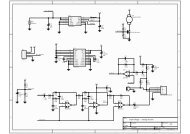
added to the accelerometer output. The circuit in
Figure 5 shows a circuit example applying an analog
linear compensation technique. In this circuit the
accelerometer temperature sensor output is added to
or subtracted from the accelerometer output.
The calibration sequence is: start at room temperature
with the 100K potentiometer set so that its wiper is at
Vref. Next, soak the accelerometer at the expected
extreme temperature and observe the direction of the
drift. Then set the switch to the non-inverting input if
the drift is negative or vice versa. Finally, adjust the
100K potentiometer while monitoring the circuit
output, until the zero g offset drift is removed.
Application Note
#AN-00MX-001
Vref
Tout
10K
10K
Aoutx or y
10K
Page 4 of 7 #AN-00MX-001
100K
SW SPDT
100K
100K
100K
100K
100K
Figure 5: Zero g Offset Temperature Compensation
Circuit
Various digital compensation techniques can be
applied using a similar concept. Digital techniques
can provide better compensation because they can
compensate for non-linear zero g offset vs.
temperature. A microcontroller or microprocessor
would perform the compensation. The acceleration
signal and the temperature signal would be digitized
using an analog to digital converter. Like in the
analog compensation, the first step is to test and
characterize the zero g drift. The purpose of the
characterization is to create a look up table or to
estimate a mathematical representation of the drift.
For example, the drift could be characterized by an
equation of the form:
Drift = a*Temperature 2 + b*Temperature + c
where a,b,c are unique constants for each
accelerometer. In normal operation the processor
calculates the output:
Compensated Output = Acceleration – Drift.
For a more detailed discussion of temperature
compensation reference MEMSIC Application Note
#AN-00MX-02.
Discussion of Tilt Applications and Minimum
Resolution
Tilt Applications: One of the most popular
applications of the MEMSIC accelerometer product
line is in tilt measurement. An accelerometer uses
the force of gravity as an input to determine the
position of an object.
A MEMSIC accelerometer is most sensitive to
changes in position, or tilt, when the accelerometer’s
axis is perpendicular to the force of gravity, or
parallel to the Earth’s surface. Similarly, when the
+
-
+5V
Aoutx or y
zero g drift
compensated

accelerometer’s axis is parallel to the force of gravity
(perpendicular to the Earth’s surface), it is least
sensitive to changes in tilt. Since a dual-axis
accelerometer from MEMSIC is not cost prohibitive
compared to a single-axis unit, as is true with nearly
all competitors’ products, using a dual-axis
accelerometer can provide high sensitivity to changes
in tilt for all angles.
Table 1 and Figure 6 illustrate the changes in the X-
and Y-axes as the unit is tilted from +90° to 0°.
Notice that when one axis has a small change in
output per degree of tilt (in mg), the second axis has a
large change in output per degree of tilt. With
triangulation, this permits low cost accurate tilt
sensing to be achieved with the MEMSIC device.
Y
MEMSIC
Top View
X
+90 0
0 0
gravity
Figure 6: Accelerometer Position Relative to Gravity
X-Axis
Orientation
To Earth’s
Surface ( 0 )
X Output
(g)
X-Axis Y-Axis
Change/
0 of tilt
(mg)
Y Output
(g)
Change/
0 of tilt
(mg)
90 1.000 0.15 0.000 17.45
85 0.996 1.37 0.087 17.37
80 0.985 2.88 0.174 17.16
70 0.940 5.86 0.342 16.35
60 0.866 8.59 0.500 15.04
45 0.707 12.23 0.707 12.23
30 0.500 15.04 0.866 8.59
20 0.342 16.35 0.940 5.86
10 0.174 17.16 0.985 2.88
5 0.087 17.37 0.996 1.37
0 0.000 17.45 1.000 0.15
Table 1: Changes in Tilt for X- and Y-Axes
Minimum Resolution: The MEMSIC accelerometer
product line is capable of resolving less than 1° of tilt
angle. The typical rms noise floor for the standard
products is specified at 1 mg Hz .
Application Note
#AN-00MX-001
When using a simple RC low pass filter to reduce the
noise by limiting the bandwidth, the noise floor of the
MEMSIC accelerometer can be calculated by the
following equation:
Noise (rms) = ( 1 mg Hz ) × ( BW × 1.
6 )
At 10 Hz, the noise will be:
Noise (rms) = ( 1 mg Hz ) × ( 4 × 1 . 6 ) = 2.5mg
The peak-to-peak value of this noise will be the rms
value x 6. 6 or 16.7mg for a 4 Hz bandwidth.
Based on the numbers in table 1 shown for a dual
axis accelerometer and the high sensitivity of the ±1g
and ±2g units, MEMSIC devices are capable of
resolving less than 1° of tilt at all possible angles.
External Filters
AC Coupling: For applications where only dynamic
accelerations (vibration) are to be measured, it is
preferable to ac couple the accelerometer output as
shown in Figure 7. The advantage of ac coupling is
that zero g offset variations from part to part and zero
g offset drift over temperature can be eliminated.
Figure 7 is a HPF (high pass filter) with a –3dB
breakpoint given by the equation: f = 1 . In
2πRC
many applications it may be desirable to have the
HPF –3dB point at a very low frequency in order to
detect very low frequency accelerations. Sometimes
the implementation of this HPF may result in
unreasonably large capacitors, and the designer must
turn to digital implementations of HPFs where very
low frequency –3dB breakpoints can be achieved.
A OUTX
A OUTY
Page 5 of 7 #AN-00MX-001
C
C
R
R
Figure 7: High Pass Filter
A OUTX
Filtered
Output
A OUTY
Filtered
Output
Low Pass Filter: An external low pass filter is
useful in low frequency applications such as tilt or
inclination. The Low Pass Filter band limits the
noise and improves the resolution achievable with
the accelerometer. When designing with MEMSIC

atiometric output accelerometers (MXRxxxx series),
it is highly recommended that an external, 200 Hz
low pass filter be used to eliminate internally
generated periodic noise that is coupled to the outputs
of the accelerometer. The low pass filter shown in
Figure 8 has a –3dB breakpoint given by the
equation: f = 1 . For the 200 Hz ratiometric
2πRC
output device filter, C=0.1µF and R=8kΩ, ±5%,
1/8W.
A OUTX
A OUTY
R
R
C
C
Figure 8: Low Pass Filter
A OUTX
Filtered
Output
A OUTY
Filtered
Output
Using MEMSIC Accelerometers in Very Low
Power Applications
In applications with power limitations, power cycling
can be used to extend the accelerometer operating
time. One important consideration when power
cycling is that the accelerometer turn on time limits
the frequency bandwidth of the accelerations to be
measured. For example, operating at 2.7V the turn on
time is 40mS. To double the operating time, a
particular application may cycle power ON for 40mS,
then OFF for 40mS, resulting in a measurement
period of 80mS, or a frequency of 12.5Hz. With a
frequency of measurements of 12.5Hz, accelerations
changes as high as 6.25Hz can be detected. Power
cycling can be used effectively in many inclinometry
applications, where inclination changes can be slow
and infrequent.
Application Note
#AN-00MX-001
Extending the Frequency Response
The response of the thermal accelerometer is a
function of the internal gas physical properties, the
natural convection mechanism and the sensor
electronics. Since the gas properties of MEMSIC's
mass produced accelerometer are uniform, a simple
circuit can be used to equally compensate all sensors.
In most applications the compensating circuit does
not require adjustment for individual units.
A simple compensating network comprising two
operational amplifiers and a few resistors and
capacitors provides increasing gain with increasing
frequency (see Figure 9). The 14.3KΩ and the
5.9KΩ resistors along with the non-polarized 0.82µF
capacitors tune the gain of the network to compensate
for the output attenuation at the higher frequencies.
The other resistors and capacitors provide noise
reduction and stability.
Aout X or Y
8.06K
0.047uF
14.3K
0.82uF
5.9K
14.3K
160K
0.01uF
0.01uF
8.06K
Page 6 of 7 #AN-00MX-001
UB
-
+
0.82uF
0.0022uF
5.9K
UA
-
+
0.047uF
Freq. Comp. Output
Figure 9: Frequency Response Extension Circuit

The accelerometer response (bottom trace), the
network response (top trace) and the compensated
response (middle trace) are shown in Figure 10. The
amplitude remains above –3db beyond 160 Hertz,
and there is useable signal well after this frequency.
Amplitude - dB
60
45
30
15
0
-15
-30
-45
-60
10 100
Frequency - Hz
1000
Figure 10: Amplitude Frequency Response
Conclusion
MEMSIC accelerometers provide the most reliable
solution in acceleration sensing at a very low cost.
Application Note
#AN-00MX-001
Page 7 of 7 #AN-00MX-001