1 Introduction - Mathematics Department - Caltech
1 Introduction - Mathematics Department - Caltech
1 Introduction - Mathematics Department - Caltech

Create successful ePaper yourself
Turn your PDF publications into a flip-book with our unique Google optimized e-Paper software.
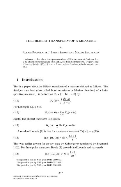
THE HILBERT TRANSFORM OF A MEASURE<br />
By<br />
ALEXEI POLTORATSKI ∗ , BARRY SIMON † AND MAXIM ZINCHENKO ‡<br />
Abstract. Let e be a homogeneous subset of R in the sense of Carleson. Let<br />
µ be a finite positive measure on R and Hµ(x) its Hilbert transform. We prove that<br />
if limt→∞ t|e∩{x | |Hµ(x)| > t}| = 0, then µs(e) = 0, where µs is the singular part<br />
of µ.<br />
1 <strong>Introduction</strong><br />
This is a paper about the Hilbert transform of a measure defined as follows. The<br />
Stieltjes transform (also called Borel transform or Markov function) of a finite<br />
(positive) measure µ is defined on C+ = {z | Im z > 0} by<br />
<br />
dµ(x)<br />
(1.1) Fµ(z) =<br />
x − z .<br />
For Lebesgue a.e. x ∈ R,<br />
(1.2) Fµ(x + i0) = lim<br />
ε↓0 Fµ(x + iε)<br />
exists. The Hilbert transform is given by<br />
(1.3) Hµ(x) = 1<br />
π Re Fµ(x + i0).<br />
A result of Loomis [8] is that for a universal constant C (µ ≡ µ(R)),<br />
(1.4) |{x : |Hµ(x)| ≥ t}| ≤ Cµ<br />
.<br />
t<br />
This was earlier proven for the a.c. case by Kolmogorov (attributed by Zygmund<br />
[16]). For finite point measures, Boole [1] proved (and Loomis rediscovered)<br />
(1.5) |{x : ±Hµ(x) ≥ t}| = µ<br />
πt .<br />
∗ Supported in part by NSF grant DMS-0800300.<br />
† Supported in part by NSF grant DMS-0652919.<br />
‡ Supported in part by NSF grant DMS-0965411.<br />
JOURNAL D’ANALYSE MATHÉMATIQUE, Vol. 111 (2010)<br />
DOI 10.1007/s11854-010-0017-0<br />
247
248 A. POLTORATSKI, B. SIMON AND M. ZINCHENKO<br />
We note that (1.5) was extended by Hruˇsčëv–Vinogradov [7] to all singular measures;<br />
see also [5, 10].<br />
Remark. We do not need an explicit value of C in (1.4). Davis [3, 4] has<br />
shown the optimal constant in (1.4) is C = 1.<br />
In distinction, for a.c. measures dµ = f dx, we have<br />
(1.6) lim<br />
t→∞ t|{x : |Hf dx(x)| ≥ t}| = 0.<br />
This follows from the facts that if f ∈ L 2 , then Hf dx ∈ L 2 (indeed, Hf dx2 = f2),<br />
that L 2 ∩ L 1 is dense in L 1 , that (1.6) is trivial if Hf dx is L 2 , and that for any<br />
θ ∈ [0, 1],<br />
(1.7)<br />
|{x : |f (x) + g(x)| > t}|<br />
≤ |{x : |f (x)| > θt}| + |{x : |g(x)| > (1 − θ)t}|.<br />
From (1.5), (1.6), and (1.7), one sees that<br />
(1.8) lim<br />
t→+∞ πt|{x : ±Hµ(x) ≥ t}| = µs,<br />
where<br />
(1.9) dµ = f dx + dµs<br />
is the Lebesgue decomposition of µ (i.e., µs is singular).<br />
In fact, a more general statement holds: for any finite complex measure µ, the<br />
measures<br />
1<br />
2 πtχ{x: |Hµ(x)|≥t} dx<br />
converge in the ∗-weak topology to the measure |dµs|; see (5.4) or [10].<br />
One can rephrase this. We recall that weak-L 1 is defined by (this is not a norm!)<br />
setting<br />
(1.10) f1,w ≡ sup<br />
t<br />
and<br />
t|{x : |f (x)| ≥ t}|<br />
(1.11) L 1 w = {f : f1,w < ∞},<br />
so (1.4) says Hµ ∈ L1 w . We also define<br />
(1.12) L 1 w;0 = f ∈ L 1 w<br />
: lim<br />
t→∞ t|{x : |f (x)| ≥ t}| = 0 .
Then (1.8) implies that<br />
THE HILBERT TRANSFORM OF A MEASURE 249<br />
(1.13) Hµ ∈ L 1 w;0 ⇔ µs(R) = 0.<br />
Our main goal is to provide a local version of this theorem for special sets<br />
singled out by Carleson [2].<br />
Definition. We say that a compact set e ⊂ R is homogeneous (with homogeneity<br />
constant δ) if there is δ > 0 such that for all x ∈ e and 0 < a < diam(e),<br />
(1.14) |e ∩ (x − a, x + a)| ≥ 2δa.<br />
Given a function f , we use f ↾ e to denote the function fχe with χe the characteristic<br />
function of e. The purpose of this paper is to prove<br />
Theorem 1.1. Let e be homogeneous and let µ be a measure on R such that<br />
Hµ ↾ e ∈ L1 w;0 . Then<br />
(1.15) µs(e) = 0.<br />
Remarks. 1. There is an analog for measures on ∂D = {z ∈ C : |z| = 1}.<br />
2. The Hilbert transform can be defined if µ, rather than being finite, satisfies<br />
<br />
−1 (1 + |x|) dµ < ∞. Indeed, Hµ can be defined up to an additive constant if<br />
<br />
2 −1 (1 + |x| ) dµ(x) < ∞. Theorem 1.1 extends to both these cases.<br />
3. It follows from the arguments in Section 2 that a converse to Theorem 1.1<br />
holds and that Hµ ↾ e ∈ L1 w;0 if and only if Hµ↾e ∈ L1 w;0 . Thus, we have a three-fold<br />
equivalence,<br />
(1.16) Hµ ↾ e ∈ L 1 w;0 ⇔ Hµ↾e ∈ L 1 w;0 ⇔ µs(e) = 0.<br />
There is a special case that is both important and one motivation for this work.<br />
Recall from [9] the following<br />
Definition. A finite measure µ on R is called reflectionless on e ⊂ R, where<br />
e is compact and of strictly positive Lebesgue measure, if and only if Hµ ↾ e = 0.<br />
There has been an explosion of recent interest about reflectionless measures<br />
due to work of Remling [12]. Clearly, the zero function lies in L1 w;0 , so we have<br />
Corollary 1.2. Let e be homogeneous, and let µ be a measure on R which is<br />
reflectionless on e. Then (1.15) holds.<br />
This result is not new. For cases where supp(µ) ⊂ e, it is due to Sodin–<br />
Yuditskii [15], with some extensions due to Gesztesy–Zinchenko [6]. Recently,
250 A. POLTORATSKI, B. SIMON AND M. ZINCHENKO<br />
Poltoratski–Remling [11] have proven a stronger result than Corollary 1.2—<br />
instead of requiring that e be homogeneous, they only need that for all x0 ∈ e,<br />
(1.17) lim sup<br />
a↓0<br />
|e ∩ (x0 − a, x0 + a)|<br />
2a<br />
> 0.<br />
If (1.17) holds for all x0 ∈ e, we call e weakly homogeneous, following [11].<br />
The property of being reflectionless is not robust in that changing µ off e usually<br />
destroys the reflectionless property. As we see in Section 2, having Hµ ↾ e in<br />
L1 w;0 is robust and explains one reason we sought this result.<br />
Our proof is quite different from [11]. We note, however, that our proof, like<br />
the one in [11], is essentially a real variable proof (we go into the complex plane<br />
but use no contour integrals), while the earlier work of [15, 6] is a complex variable<br />
argument.<br />
We mention that Corollary 1.2 (and so Theorem 1.1) does not hold for arbitrary<br />
e. Nazarov–Volberg–Yuditskii [9] have examples of reflectionless measures on<br />
their supports where (1.17) fails and that have a singular component.<br />
We mention another special case of Theorem 1.1.<br />
Corollary 1.3. Let e be a homogeneous set in R. Let µ be a measure on R<br />
such that there is a set A satisfying<br />
(i) |A| = 0,<br />
(ii) µ(R \ A) = 0,<br />
(iii) A is closed and A ⊂ e.<br />
Suppose Hµ ↾ e ∈ L1 w;0 . Then µ = 0.<br />
We need a strengthening of this special case.<br />
Theorem 1.4. Let e be a homogeneous set in R. There is a constant C1<br />
depending only on e such that for any measure µ obeying (i)–(iii) of Corollary 1.3,<br />
we have<br />
(1.18) µ(e) ≤ C1 lim inf<br />
t→∞ t|{x ∈ e : |Hµ(x)| ≥ t}|.<br />
Remarks. 1. In fact, C1 is only δ-dependent; explicitly, one can take<br />
(1.19) C1 = 1536π3<br />
δ2 .<br />
We have made no attempt to optimize this constant and, indeed, have made choices<br />
to simplify the arithmetic. The δ −2 may be optimal; it certainly seems that δ −1 is<br />
not possible.<br />
2. There is also a strengthening of Theorem 1.1 of this same form.
THE HILBERT TRANSFORM OF A MEASURE 251<br />
We can say more about weakly homogeneous sets, that is, ones that obey<br />
(1.17), and thereby illuminate and limit Theorem 1.1.<br />
Theorem 1.5. Let e be a compact weakly homogeneous set and µ a measure<br />
on R such that Hµ ↾ e ∈ L 1 w;0 . Then for all x0 ∈ e,<br />
(1.20) µ({x0}) = 0,<br />
that is, µ has no pure point masses in e.<br />
Theorem 1.6. There exists a weakly homogeneous set e containing the classical<br />
Cantor set, such that if µ is the conventional Cantor measure, Hµ ↾ e ∈ L 1 w;0 .<br />
In particular, Theorem 1.1 does not extend to weakly homogeneous sets.<br />
While the gap between homogeneous and weakly homogeneous sets is not<br />
large, we can extend Theorem 1.1 to partly fill it in. We call a set e nonuniformly<br />
homogeneous if it is closed and<br />
(1.21) lim inf (2a)<br />
a↓0<br />
−1 |e ∩ (x − a, x + a)| > 0<br />
for all x ∈ e.<br />
Theorem 1.7. Let e be non-uniformly homogeneous and let µ be a measure<br />
on R such that Hµ ↾ e ∈ L1 w;0 . Then<br />
(1.22) µs(e) = 0.<br />
In fact, we obtains this from a stronger result. We emphasize that in the next<br />
theorem, e is not assumed closed.<br />
Theorem 1.8. Let e be a Borel set in R and µ a finite measure such that<br />
Hµ ↾ e ∈L1 w;0 . Then<br />
<br />
(1.23) µs {x ∈ e : lim inf (2a) −1 |e ∩ (x − a, x + a)| > 0} = 0.<br />
a↓0<br />
This is to be compared with the result of Poltoratski–Remling [11] that if e is<br />
Borel and Hµ ↾ e = 0, then<br />
<br />
(1.24) µs {x ∈ e : lim sup (2a) −1 |e ∩ (x − a, x + a)| > 0} = 0,<br />
a↓0<br />
and the statement (which follows from our proof of Theorem 1.5) that if µpp is the<br />
pure point part of µ, then if Hµ ↾ e ∈ L 1 w;0 ,<br />
µpp<br />
<br />
{x ∈ e : lim sup (2a) −1 |e ∩ (x − a, x + a)| > 0} = 0.<br />
a↓0
252 A. POLTORATSKI, B. SIMON AND M. ZINCHENKO<br />
Moreover, we note that the example in Theorem 1.6 shows that in Theorem 1.8,<br />
we cannot replace (1.23) by (1.24).<br />
In Section 2, we reduce the proof of Theorem 1.1 to proving Theorem 1.4. In<br />
Section 3, we prove Theorem 1.4. In proving Theorem 1.4, we first show that if<br />
[a, b] is an interval on which |Fµ(x+i0)| ≥ t, then |Fµ(x+i(b−a))| ≥ t/8π 2 . Then<br />
we use this to prove that on most of [a−(b−a), a] and [b, b + (b−a)], |Fµ(x + i0)|<br />
is a significant fraction of t, which is the key to the proof. In Section 4, we prove<br />
Theorems 1.5 and 1.6. In Section 5, we prove Theorem 1.8, and so Theorem 1.7.<br />
Acknowledgement. We thank Jonathan Breuer and Yoram Last for useful<br />
discussions.<br />
2 Reduction to Theorem 1.4<br />
In this section, we show that Theorem 1.4 implies Theorem 1.1.<br />
Proposition 2.1. Let µ have the form (1.9). Then for any set e ⊂ R,<br />
(2.1) Hµ ↾ e ∈ L 1 w;0 ⇔ Hµs ↾ e ∈ L1 w;0 .<br />
In particular, we need only prove Theorem 1.1 for purely singular measures to get<br />
it for all measures.<br />
Remark. This shows the advantage of working with L1 w;0 . Purely singular<br />
measures are never reflectionless (for |{x : Fµ(x + i0) = 0}| = 0 and thus,<br />
Im Fµ(x + i0) > 0 a.e. on e if Hµ ↾ e = 0).<br />
Proof. By (1.7) with θ = 1<br />
2 ,L1 w;0 is a vector space. SinceHµ−Hµs =Hf dµ∈L 1 w;0 ,<br />
by (1.6), we get (2.1) immediately. <br />
Proposition 2.2. Let e be a closed set. Let µ be a measure with µ(e) = 0.<br />
Then<br />
(2.2) Hµ ↾ e ∈ L 1 w;0.<br />
Proof. Let µm = µ ↾ {x : dist(x, e) ≥ m −1 }. Then for x ∈ e,<br />
1<br />
(2.3) Hµm (x) =<br />
π<br />
so<br />
dµm(y)<br />
y − x ,<br />
(2.4) Hµm ↾ e∞ ≤ m<br />
π µm;
hence Hµm ∈ L1w;0 .<br />
By (1.7) with θ = 1<br />
2 , for any m,<br />
(2.5)<br />
lim sup<br />
t→∞<br />
THE HILBERT TRANSFORM OF A MEASURE 253<br />
t|{x ∈ e : |Hµ(x)| ≥ t}| ≤ 2 lim sup<br />
t→∞<br />
≤ 2Cµ − µm,<br />
t|{x ∈ e : |Hµ−µm (x)| ≥ t}|<br />
where C is the constant in (1.4).<br />
Since (2.5) holds for all m and µ − µm → 0 (since µ(e) = 0), we conclude<br />
Hµ ↾ e ∈ L1 w;0 . <br />
Proposition 2.3. Let e be a closed set. Let ν = µ ↾ e, that is, ν(A) = µ(e∩A).<br />
Then<br />
(2.6) Hν ↾ e ∈ L 1 w;0 ⇔ Hµ ↾ e ∈ L 1 w;0 .<br />
In particular, it suffices to prove Theorem 1.1 for purely singular measures supported<br />
on e.<br />
Proof. Let η = µ − ν. By Proposition 2.2,<br />
(2.7) Hµ ↾ e − Hν ↾ e = Hη ↾ e ∈ L 1 w;0.<br />
Since L 1 w;0<br />
is a vector space, (2.7) implies (2.6). <br />
Proof of Theorem 1.1 given Theorem 1.4. By Proposition 2.3, we can<br />
suppose µ is purely singular and supported by e. Thus, there exists A∞ ⊂ e with<br />
|A∞| = 0, so µ(R \ A∞) = 0.<br />
By regularity of measures, we can find An ⊂ An+1 ⊂ ··· ⊂ A∞ with each An<br />
closed, and so<br />
(2.8) µ(A∞ \ An) → 0.<br />
Define µn = µ ↾ An and νn = µ − µn. By (1.7) with θ = 1<br />
2 , Hµ ↾ e ∈ L1 w;0 , and<br />
(1.4),<br />
(2.9)<br />
lim sup<br />
t→∞<br />
t|{x ∈ e : |Hµn (x)| ≥ t}| ≤ 2 lim sup t|{x ∈ e : |Hνn (x)| ≥ t}|<br />
t→∞<br />
≤ 2Cµ(A∞ \ An).<br />
Now An satisfies (i)–(iii) for µn, so by (1.18),<br />
(2.10) µ(An) = µn(e) ≤ 2CC1µ(A∞ \ An).<br />
As n → ∞, µ(An) → µs(e) while, by (2.8), µ(A∞ \ An) → 0. So µs(e) = 0.
254 A. POLTORATSKI, B. SIMON AND M. ZINCHENKO<br />
3 Proof of Theorem 1.4<br />
Throughout this section, where we prove Theorem 1.4 and so complete the proof<br />
of Theorem 1.1, we suppose e is homogeneous with homogeneity constant δ, and<br />
µ is a measure for which there exists A ⊂ e satisfying covditions (i)–(iii) of Corollary<br />
1.3. In particular, since µ is singular, for a.e. x ∈ R,<br />
(3.1) Fµ(x + i0) = πHµ(x).<br />
We consider Fµ throughout.<br />
The key is to prove that for all large t,<br />
(3.2)<br />
<br />
<br />
x ∈ e : |Fµ(x + i0)| > δ <br />
δ<br />
t ≥<br />
128π2 24 |{x : |Fµ(x + i0)| > t}|.<br />
We do this by showing that if I is an interval in R\A where |Fµ(x+i0)| > t, then at<br />
most points of the two touching intervals of the same size, |Fµ| ≥ δt/128π 2 . We do<br />
this in two steps. We show that at points over I with Im z = |I|, F(z) is comparable<br />
to t and use that to control F on the touching intervals. A Vitali covering map<br />
argument then boosts that up to the full sets. We need<br />
Proposition 3.1. Let<br />
(3.3) I = [c − a, c + a]<br />
be an interval contained in<br />
(3.4) {x : |Fµ(x + i0)| ≥ t}.<br />
Then<br />
(3.5) |Fµ(c + a + 2ia)| ≥ t<br />
8π 2.<br />
Proof. Fµ lies in weak L1 and is bounded off a compact subset of R. For<br />
z ∈ C+, let<br />
<br />
(3.6) G(z) = Fµ(z)/i.<br />
Then G has locally L1 boundary values on R and is bounded off a compact set, so<br />
if z = x + iy,<br />
(3.7) G(z) = 1<br />
<br />
yG(λ + i0) dλ<br />
π (x − λ) 2 .<br />
+ y2
Now arg(G) ∈ [− π<br />
4<br />
THE HILBERT TRANSFORM OF A MEASURE 255<br />
π , 4 ], so on R,<br />
(3.8) Re G(λ + i0) ≥ 0.<br />
On I, arg(G) = ± π<br />
4 , and so for λ ∈ I,<br />
(3.9) Re G(λ + i0) ≥ t/2.<br />
Thus, by (3.7), (3.8) and (3.9),<br />
Re G(c + a + 2ia) ≥ 1<br />
<br />
2a Re G(λ + i0)<br />
π I (c + a − λ) 2 dλ<br />
+ (2a) 2<br />
≥ 1 (2a)<br />
π<br />
2√t/2 (2a) 2 1 <br />
(3.10)<br />
≥ t/2,<br />
+ (2a) 2 2π<br />
so<br />
(3.11) |Fµ(c + a + 2ia)| ≥ (Re G(c + a + 2ia)) 2 ≥ t<br />
8π 2.<br />
Lemma 3.2. Fix t0 > 0 and let<br />
(3.12) Ft0 (z) =<br />
Then Im Ft0 > 0 on C+, and<br />
F(z)<br />
1 + 1<br />
t0 F(z).<br />
(3.13) {x : |F(x + i0)| > t0} = {x : Ft0 (x + i0) > t0/2}.<br />
Remark. Ft0 is the Stieltjes transform of a measure associated with a rank<br />
one perturbation (see, e.g., [14, Sect. 11.2]), but that plays no direct role here.<br />
Proof. The invertible map<br />
z<br />
(3.14) H(z) =<br />
1 + z/t0<br />
maps C+ to C+ and (t0,∞) ∪ {∞} ∪ (−∞,−t0) to ( t0<br />
2 ,∞). <br />
For any x > 0, define<br />
(3.15) Ŵs = {x : |F(x + i0)| > s}.<br />
Proposition 3.3. Fix t > 0 and let<br />
(3.16) t0 =<br />
δ<br />
t.<br />
128π2
256 A. POLTORATSKI, B. SIMON AND M. ZINCHENKO<br />
Suppose<br />
(3.17) I = [c − a, c + a] ⊆ Ŵt,<br />
and let<br />
(3.18) Ĩ = [c + a, c + 3a]<br />
be the touching interval of the same size as I. Then<br />
δ<br />
(3.19) |Ĩ \ Ŵt0 | ≤ aδ =<br />
2 |I|.<br />
Proof. By the lemma for x real,<br />
(3.20) χŴt 0 (x) = 1 − 1<br />
π<br />
arg(Ft0 (x + i0) − t0/2),<br />
which is the boundary value of a bounded harmonic function.<br />
Let<br />
(3.21) z0 = c + a + 2ia.<br />
Then<br />
(3.22)<br />
(3.23)<br />
<br />
arg Ft0 (z0) − t0<br />
<br />
F(z0) − t0/2 − F(z0)/2<br />
= arg<br />
2<br />
1 + 1<br />
t0 F(z0)<br />
<br />
<br />
F(z0)/t0 − 1<br />
= arg<br />
= arg 1 −<br />
F(z0)/t0 + 1<br />
By Proposition 3.1,<br />
<br />
<br />
<br />
F(z0) <br />
<br />
<br />
since δ ≤ 1. Thus,<br />
<br />
<br />
(3.24) <br />
2 <br />
<br />
F(z0)/t0<br />
+ 1<br />
≤<br />
If |w| ≤ 1 for w ∈ C, then<br />
t0<br />
≥ t<br />
8π 2 t0<br />
= 16<br />
δ<br />
≥ 16<br />
2 2<br />
≤ < 1.<br />
|F(z0)/t0| − 1 15<br />
(3.25) arg(1 + w) ≤ arcsin(|w|) ≤ π<br />
2 |w|<br />
2<br />
F(z0)/t0 + 1<br />
(sin(y) ≥ (2y)/π for y ∈ [0,π/2] implies for x ∈ [0, 1], arcsin x ≤ π<br />
2 x). By (3.22),<br />
<br />
(3.26) arg Ft0 (z0) − t0<br />
<br />
≤<br />
2<br />
8π3t0 t − 8π2 .<br />
t0<br />
<br />
.
THE HILBERT TRANSFORM OF A MEASURE 257<br />
Thus, if χŴt 0 (z) is the harmonic function whose boundary value is χŴt 0 (x), we<br />
find, by (3.20), that<br />
(3.27) π(1 − χŴt (z0)) ≤<br />
0 8π3t0 t − 8π2 .<br />
t0<br />
By a Poisson formula with z0 = x0 + iy0 as in (3.21),<br />
<br />
π(1 − χŴt (z0)) =<br />
0<br />
R\Ŵt0 y0 dλ<br />
(λ − x0) 2 + y2 (3.28)<br />
0<br />
≥ 1 |Ĩ \ Ŵt0<br />
2<br />
|<br />
(3.29)<br />
,<br />
|I|<br />
since on Ĩ, the minimum of y0/((λ − x0) 2 + y2 0 ) is 1/(2|I|).<br />
Thus, by (3.27) and (3.29),<br />
(3.30) |Ĩ \ Ŵt0 | ≤ 16π3t0 t − 8π2 |I|.<br />
t0<br />
Since 8π2 t0<br />
t<br />
1 ≤ 16 ,<br />
16π 3 t0<br />
t<br />
1 − 8π2 t0<br />
t<br />
≤ 256π3 t0<br />
15 t<br />
= 4π<br />
15<br />
δ δ<br />
≤<br />
2 2 ,<br />
and (3.30) implies (3.19). <br />
Proposition 3.4. Under the notation of Proposition 3.3, let<br />
(3.31) I ♯ = [c − 3a, c + 3a]<br />
and suppose<br />
(3.32) e ∩ I = ∅<br />
and<br />
(3.33) a ≤ diam(e).<br />
Then<br />
(3.34) |Ŵt0 ∩ e ∩ I♯ | ≥ δ<br />
2 |I|.<br />
Proof. Pick x0 ∈ e ∩ I. Suppose x0 ≥ c. If not, we pick Ĩ to be the third of I ♯<br />
below I instead of the choice here. By homogeneity,<br />
(3.35) |e ∩ (x0 − a, x0 + a)| ≥ 2aδ = δ|I|
258 A. POLTORATSKI, B. SIMON AND M. ZINCHENKO<br />
and the intersection lies in I ∪ Ĩ. Thus,<br />
(3.36) |Ŵt0 ∩ e ∩ I♯ | ≥ |e ∩ (x0 − a, x0 + a)| − |(I ∪ Ĩ) \ Ŵt0 |.<br />
Since I ⊂ Ŵt ⊂ Ŵt0 ,<br />
δ<br />
(3.37) |(I ∪ Ĩ) \ Ŵt0 | = |Ĩ \ Ŵt0 | ≤<br />
2 |I|<br />
by (3.19); (3.35) and (3.36) imply (3.34). <br />
Proof of Theorem 1.4. Suppose µ = 0. On R \ A, Fµ(x + i0) is continuous<br />
and real, so {x : |Fµ(x + i0)| > t} is open, and hence a countable union of maximal<br />
disjoint open intervals.<br />
Let I = [c − a, c + a] be the closure of any such interval. On R \ A, Fµ(x) has<br />
(3.38) F ′ <br />
µ(x) =<br />
dµ(x)<br />
> 0.<br />
(y − x) 2<br />
If Fµ > t on I, c + a must be in A or else Fµ(c + a) < ∞ and Fµ(c + a + ε) ∈ Ŵt<br />
for ε small (so I is not maximal). Similarly, if Fµ < −t on I, c − a ∈ A. Thus,<br />
I ∩ A = ∅, so I ∩ e = ∅.<br />
Let<br />
(3.39) T = πCµ<br />
diam(e) ,<br />
where C is the constant in (1.4). Then for t > T, |Ŵt| ≤ diam(e), so a ≤ diam(e).<br />
Thus, by Proposition 3.4,<br />
(3.40) |Ŵt0 ∩ e ∩ I♯ | ≥ δ<br />
2 |I|.<br />
Clearly, the I’s and so the (I ♯ ) int ’s are an open cover of Ŵt\A. Thus, by the Vitali<br />
covering theorem (see Rudin [13, Lemma 7.3]), we can find a subset of mutually<br />
}) such that<br />
disjoint I ♯ ’s (call them {I ♯<br />
j<br />
(3.41) |Ŵt| ≤ 4 <br />
j<br />
|I ♯<br />
j<br />
By the disjointness, with t0 given by (3.16),<br />
<br />
|Ŵt0 ∩ e| ≥<br />
j<br />
≥ δ<br />
2<br />
<br />
| ≤ 12 |Ij|.<br />
|I ♯<br />
j ∩ Ŵt0 ∩ e|<br />
<br />
|Ij| (by (3.34))<br />
j<br />
j
Thus,<br />
THE HILBERT TRANSFORM OF A MEASURE 259<br />
lim inf<br />
t→∞<br />
Therefore, by (1.8) and (3.1),<br />
≥ δ<br />
24 |Ŵt| (by (3.41)).<br />
t0|Ŵt0 ∩ e| ≥ lim inf<br />
t→∞<br />
δ<br />
24<br />
δ<br />
t|Ŵt|.<br />
128π2 lim inf<br />
t→∞ t|{x ∈ e : |Hµ(x)| > t}| ≥ δ2<br />
3072π 2<br />
2(µ(A))<br />
,<br />
π<br />
which is (1.18)/(1.19). <br />
4 Weakly homogeneous sets<br />
Proof of Theorem 1.5. For x0 ∈ e and ε > 0, write<br />
(4.1) µ = µ1 + µ2 + µ3<br />
with µ1 = µ ↾ {x0}, µ2 = µ ↾ [(x0 − ε, x0 + ε) \ {x0}], µ3 = µ ↾ R \ (x0 − ε, x0 + ε);<br />
and by (1.7), note that<br />
(4.2)<br />
|{x ∈ e; |x − x0| < ε<br />
2 : |Hµ1 (x)| > 3t}|<br />
≤|{x ∈ e : |Hµ(x)| > t}| + |{x : |Hµ2 (x)| > t}|<br />
+ |{x; |x − x0| < ε<br />
2 : |Hµ3 (x)| > t}|.<br />
By hypothesis, the first term on the right of (4.2) is o(1/t). Since |Hµ3 (x)| ≤<br />
2/ε, the third term is o(1/t). By (1.4), the second term is bounded by<br />
Cµ((x0 − ε, x0 + ε) \ {x0})/t.<br />
So long as t > 2µ({x0})<br />
3πε , the left side of (4.2) is |e ∩ (x0 − 2µ({x0})<br />
3πt , x0 + 2µ({x0})<br />
3πt )|.<br />
Thus, if<br />
(4.3) C(x0) = lim sup (2s)<br />
s↓0<br />
−1 |e ∩ (x0 − s, x0 + s)|,<br />
(4.2) implies that<br />
(4.4)<br />
4C(x0)µ({x0})<br />
3π<br />
≤ Cµ((x0 − ε, x0 + ε) \ {x0})<br />
for any ε. Since ∩[(x0 − 1<br />
m , x0 + 1<br />
m ) \ {x0}] = ∅, the right side of (4.4) goes to zero<br />
as ε ↓ 0, and we conclude that µ({x0}) = 0.
260 A. POLTORATSKI, B. SIMON AND M. ZINCHENKO<br />
To prove Theorem 1.6, we need to describe some sets connected with the Can-<br />
tor set. Let K1 be the two connected closed sets K1,1, K1,2 obtained from [0, 1] by<br />
removing the middle third. At level n, we have 2 n intervals {Kn,j} 2n<br />
j=1<br />
, each with<br />
|Kn,j| = 3 −n so |Kn| = ( 2<br />
3 )n . The Cantor set, of course, is K∞ = ∩Kn. The Cantor<br />
measure is determined by<br />
(4.5) µ(Kn,j) = 1<br />
2 n.<br />
We order I = {(n, j) : n = 1, 2,..., j = 1, 2,...,2 n } with lexigraphic order and<br />
use (n, j + 1) for the obvious pair if j < 2 n and to be (n + 1, 1) if j = 2 n . Similarly,<br />
(n, j − 1) is (n − 1, 2 n−1 ) if j = 1.<br />
Let E1 be the middle closed third of [0, 1] \ K1, so |E1| = 1/9. Let E2 be the<br />
two middle thirds of the two gaps in K1 \ K2; Em has 2 m−1 closed intervals of size<br />
1/3 m+1 . There is a unique affine order preserving map of [0, 1] to Kn,j. Let En,j,m be<br />
the image of Em under this map, so En,j,m has 2 m−1 intervals, each of size 1/3 n+m+1 ,<br />
that is,<br />
(4.6) |En,j,m| = 2 m−1 /3 n+m+1 .<br />
We want to pick a positive integer m(n, j) for each (n, j) ∈ I so that<br />
(4.7) m(n, j + 1) > m(n, j),<br />
and we define<br />
(4.8) k(n, j) = n + m(n, j).<br />
Given such a choice, we define<br />
(4.9) e = K∞ ∪ <br />
n,j∈I<br />
En,j,m(n,j).<br />
Our goal will be to prove e is always weakly homogeneous, and that if m(n, j)<br />
grows fast enough, then Hµ ↾ e is in L 1 w;0 .<br />
Lemma 4.1. For any choice of m(n, j), e is weakly homogeneous. Indeed, for<br />
any x0 ∈ e,<br />
(4.10) lim sup(2δ)<br />
δ↓0<br />
−1 |e ∩ (x0 − δ, x0 + δ)| ≥ 1/10.<br />
(4.11)<br />
Proof. Let<br />
˜En,j = En,j,m(n,j).
THE HILBERT TRANSFORM OF A MEASURE 261<br />
If x0 ∈ ˜En,j, which is a closed interval, for all small δ, (2δ) −1 | ˜En,j∩(x0−δ, x0+δ)| =<br />
1<br />
2 or 1, depending on whether x0 is a boundary or an interior point. So (4.10) is<br />
certainly true.<br />
Thus, we need only consider x0 ∈ K∞. Fix x0 ∈ K∞. For each n, x0 ∈ Kn,<br />
and so in Kn,jn for some jn. Let kn ≡ k(n, jn). On level kn, x0 is contained in some<br />
interval Kkn,ℓ of size 3−kn , and on one side or the other there is an interval of size<br />
3−kn−1 in ˜En,jn in a touching gap. Let<br />
(4.12) δn = 5<br />
3 3−kn .<br />
Then (x0 − δn, x0 + δn) contains this interval in ˜En,jn . Thus,<br />
(4.13) (2δn) −1 |e ∩ (x0 − δn, x0 + δn)| ≥ 3−kn−1<br />
2δn<br />
= 1<br />
10 .<br />
Since δn → 0 as n → ∞, (4.10) holds. <br />
For each (n, j), we wish to define<br />
(4.14) µn,j = µ ↾ Kn,j ∪ Kn,j−1, ˜µn,j = µ − µn,j,<br />
that is, single out the part of the Cantor measure near Kn,j, and so near En,j. We<br />
define<br />
(4.15) Fn,j = Fµn,j , ˜Fn,j = F ˜µn,j .<br />
Lemma 4.2. On <br />
(ñ,˜j)≤(n,j) ˜E ñ,˜j, we have<br />
(4.16) | ˜Fn,j| ≤ 3 k(n,j−1) .<br />
Proof. Since ˜µn,j ≤ 1, we have<br />
(4.17) | ˜Fn,j(x)| ≤ dist(x, K∞ \ Kn,j−1 ∪ Kn,j)) −1 .<br />
By construction,<br />
(4.18) dist( ˜E ñ,˜j, K∞) = 3 −k(ñ,˜j)−1 ,<br />
so if (ñ, ˜j) < (n, j − 1), then for x ∈ ˜E ñ,˜j,<br />
(4.19) | ˜Fn,j(x)| ≤ 3 k(ñ,˜j)+1 ≤ 3 k(n,j−1) ,<br />
since m(ñ, ˜j) + 1 < m(n, j − 1) implies k(ñ, ˜j) + 1 ≤ k(n, j − 1).<br />
On the other hand, since we have removed Kn,j−1 ∪ Kn,j,<br />
(4.20) dist( ˜En,j ∪ ˜En,j−1, K∞ \ (Kn,j ∪ Kn,j−1)) ≥ 3 −n .
262 A. POLTORATSKI, B. SIMON AND M. ZINCHENKO<br />
Thus, for x in ˜En,j ∪ ˜En,j−1, we have<br />
(4.21) | ˜Fn,j(x)| ≤ 3 n ≤ 3 k(n,j−1) ,<br />
proving (4.16) on the claimed set. <br />
Proof of Theorem 1.6. We construct e by using the above construction<br />
where m(n, j) is picked inductively, so that<br />
(4.22) k(n, j + 1) = 3k(n, j).<br />
By Lemma 4.1, e is weakly homogeneous.<br />
Let<br />
(4.23) 3 k(n,j−1) < t ≤ 3 k(n,j) .<br />
Since Fµ = Fn,j + ˜Fn,j, by (1.7),<br />
(4.24)<br />
2t|{x ∈ e : |Fµ(x)| ≥ 2t}| ≤2t|{x : |Fn,j(x)| ≥ t}|<br />
+ 2t|{x ∈ e : | ˜Fn,j(x)| ≥ t}|.<br />
By Boole’s equality (1.5), the first term on the right side of (4.24) is bounded<br />
by<br />
(4.25) 4(µn,j−1(R) + µn,j(R)) ≤ 4[2 −n + 2 · 2 −n ] = 12 · 2 −n<br />
(where we need the 2 · 2−n if j = 1).<br />
By Lemma 4.2, the second term is bounded by<br />
<br />
k(n,j)<br />
(4.26) 2 · 3<br />
By (4.6),<br />
(4.27) | ˜En,j| =<br />
therefore, since<br />
(4.28)<br />
(4.29)<br />
(ñ,˜j)≥(n,j+1)<br />
1<br />
2 n+1 3<br />
∞<br />
ℓ <br />
2 2<br />
= 3<br />
3 3<br />
ℓ=ℓ0<br />
(4.26) ≤ 3 k(n,j) 2 −n<br />
<br />
2<br />
3<br />
By (4.22) and ( 3<br />
2 )3 = 27<br />
8 > 3, we see that<br />
(4.30) (4.26) ≤ 2 −n .<br />
|E ñ,˜j|.<br />
k(n,j) 2<br />
,<br />
3<br />
ℓ0<br />
,<br />
k(n,j+1)<br />
.
THE HILBERT TRANSFORM OF A MEASURE 263<br />
Thus, if t obeys (4.23), then by (4.24), (4.25), and (4.30),<br />
(4.31) 2t|{x ∈ e : |Fµ(x)| ≥ t}| ≤ 13 · 2 −n .<br />
Since n → ∞ as t → ∞, we see that Fµ ↾ e ∈ L1 w;0 . <br />
5 Non-uniformly homogeneous sets<br />
Our goal in this section is to prove Theorem 1.8 and then also Theorem 1.7. For<br />
any Borel set e, define<br />
(5.1) en =<br />
<br />
x ∈ e : ∀ a < 1<br />
n<br />
<br />
2a<br />
, |(x − a, x + a) ∩ e| ≥ .<br />
n<br />
Proposition 5.1. Letµbe a measure with µ(R\en) =0. SupposeHµ↾e∈L 1 w;0 .<br />
Then µs = 0.<br />
Proof. First note that en is closed, for if xm → x and |(xm−a, xm +a)∩e| ≥ 2a<br />
n ,<br />
then for all m,<br />
(5.2) |(x − a, x + a) ∩ e| ≥ 2a<br />
n<br />
− 2|x − xm|,<br />
so x ∈ en. Applying Theorem 1.1 to dµ and compact homogeneous sets<br />
en ∩ [−N, N] for all N ≥ 1, we get the result. <br />
Because e is not closed, we cannot use Propositions 2.2 and 2.3 to restrict to<br />
em. Instead we need<br />
Proposition 5.2. Let µ and ν be two measures on R whose singular parts are<br />
mutually singular. Then for all c > 0,<br />
(5.3) t|{x : |Hµ(x)| ≥ t} ∩ {x : |Hν(x)| ≥ ct}| → 0<br />
as t → ∞.<br />
Remark. This result is essentially in Poltoratski [10] (see the last set out formula<br />
in the proof of Theorem 2 in that paper), so we only sketch the proof.<br />
Sketch. Suppose first that c = 1. We begin with what is essentially Theorem<br />
1 of [10], that for any positive measure µ, as t → ∞,<br />
(5.4)<br />
1<br />
2 πtχ{x:|Hµ(x)|≥t} dx w<br />
−→ dµs
264 A. POLTORATSKI, B. SIMON AND M. ZINCHENKO<br />
in the weak-∗ topology. By (1.6) and (1.7), it suffices to prove this for µ = µs. In<br />
that case, if µ (α) is the measure with Stieltjes transform,<br />
(5.5) Fα(z) =<br />
then ([5, 10])<br />
(πt) −1<br />
−(πt) −1<br />
F(z)<br />
1 + αF(z) ,<br />
(dµα(x)) dα = χ{x:|Hµ(x)|≥t} dx,<br />
w<br />
so (5.4) follows from dµα → dµ as |α| → 0.<br />
By (1.8), if µ (t) is the measure on the left side of (5.4), then<br />
(5.6) µ (t) → µs.<br />
By (5.4),<br />
(5.7) µ (t) (t)<br />
w<br />
− ν −→ µs − νs,<br />
so<br />
(5.8) lim inf µ (t) − ν (t) ≥ µs − νs = µs + νs<br />
by the assumed mutual singularity.<br />
But<br />
(5.9) µ (t) − ν (t) = µ (t) + ν (t) − π(lhs of (5.3));<br />
(5.6) and (5.8) then imply (5.3) for c = 1.<br />
This implies the result for c ≥ 1 and then, by symmetry, for all c > 0. <br />
Proof of Theorem 1.8. For each n, define<br />
(5.10) µn = µ ↾ en, νn = µ − µn.<br />
By (1.7),<br />
(5.11)<br />
|{x ∈ e : |Hµn (x)| ≥ 2t}| ≤ |{x ∈ e : |Hµ(x)| ≥ t}|<br />
+ |{x : |Hµn (x)| ≥ 2t, |Hνn (x)| ≥ t}|.<br />
By the hypothesis, the first term on the right is o(1/t) and, by Proposition 5.2,<br />
the second is o(1/t). Thus, Hµn ↾ e ∈ L1 w;0 , and it follows from Proposition 5.1 that<br />
(µn)s = 0, that is, µs(en) = 0.<br />
Since<br />
<br />
en = x ∈ e : | lim inf (2a)<br />
a↓0<br />
−1 |e ∩ (x − a, x + a)| > 0 ,<br />
n<br />
we have (1.23).
THE HILBERT TRANSFORM OF A MEASURE 265<br />
REFERENCES<br />
[1] G. Boole, On the comparison of transcendents, with certain applications to the theory of definite<br />
integrals, Philos. Trans. Roy. Soc. London 147 (1857), 745–803.<br />
[2] L. Carleson, On H ∞ in multiply connected domains, in Proceedings of a Conference on Harmonic<br />
Analysis in Honor of Antoni Zygmund, Vol. I, II (Chicago, IL, 1981), Wadsworth, Belmont, CA,<br />
1983, pp. 349–372.<br />
[3] B. Davis, On the distributions of conjugate functions of nonnegative measures, Duke Math. J. 40<br />
(1973), 695–700.<br />
[4] B. Davis, On the weak type (1, 1) inequality for conjugate functions, Proc. Amer. Math. Soc. 44<br />
(1974), 307–311.<br />
[5] R. del Rio, S. Jitomirskaya, Y. Last and B. Simon, Operators with singular continuous spectrum,<br />
IV. Hausdorff dimensions, rank one perturbations, and localization, J. Analyse Math. 69 (1996),<br />
153–200.<br />
[6] F. Gesztesy and M. Zinchenko, Local spectral properties of reflectionless Jacobi, CMV, and<br />
Schrödinger operators, J. Differential Equations 246 (2009), 78–107.<br />
[7] S. V. Hruˇsčëv and S. A. Vinogradov, Free interpolation in the space of uniformly convergent<br />
Taylor series, in Complex Analysis and Spectral Theory (Leningrad, 1979/1980), Lecture Notes<br />
in Math. 864, Springer, Berlin–New York, 1981, pp. 171–213.<br />
[8] L. H. Loomis, A note on the Hilbert transform, Bull. Amer. Math. Soc. 52 (1946), 1082–1086.<br />
[9] F. Nazarov, A. Volberg and P. Yuditskii, Reflectionless measures with a point mass and singular<br />
continuous component, preprint.http://arxiv.org/abs/0711.0948<br />
[10] A. Poltoratski, On the distributions of boundary values of Cauchy integrals, Proc. Amer. Math.<br />
Soc. 124 (1996), 2455–2463.<br />
[11] A. Poltoratski and C. Remling, Reflectionless Herglotz functions and Jacobi matrices, Comm.<br />
Math. Phys. 288 (2009), 1007–1021.<br />
[12] C. Remling, The absolutely continuous spectrum of Jacobi matrices, preprint.<br />
[13] W. Rudin, Real and Complex Analysis, 3rd edition, McGraw-Hill, New York, 1987.<br />
[14] B. Simon, Trace Ideals and Their Applications, 2nd edition, Amer. Math. Soc., Providence, R.I.,<br />
2005.<br />
[15] M. Sodin and P. Yuditskii, Almost periodic Jacobi matrices with homogeneous spectrum, infinitedimensional<br />
Jacobi inversion, and Hardy spaces of character-automorphic functions, J. Geom.<br />
Anal. 7 (1997), 387–435.<br />
[16] A. Zygmund, Trigonometric Series. Vol. I, II, 3rd edition, Cambridge University Press, Cambridge,<br />
2002.<br />
Alexei Poltoratski<br />
MATHEMATICS DEPARTMENT<br />
TEXAS A&M UNIVERSITY<br />
COLLEGE STATION, TX 77843, USA<br />
email: alexei@math.tamu.edu<br />
Barry Simon and Maxim Zinchenko<br />
MATHEMATICS 253-37<br />
CALIFORNIA INSTITUTE OF TECHNOLOGY<br />
PASADENA, CA 91125, USA<br />
email: bsimon@caltech.edu and maxim@caltech.edu<br />
(Received December 9, 2008)