Systematic development of coarse-grained polymer models Patrick ...

3.4. Force-extension Results 25
3.4 Force-extension Results
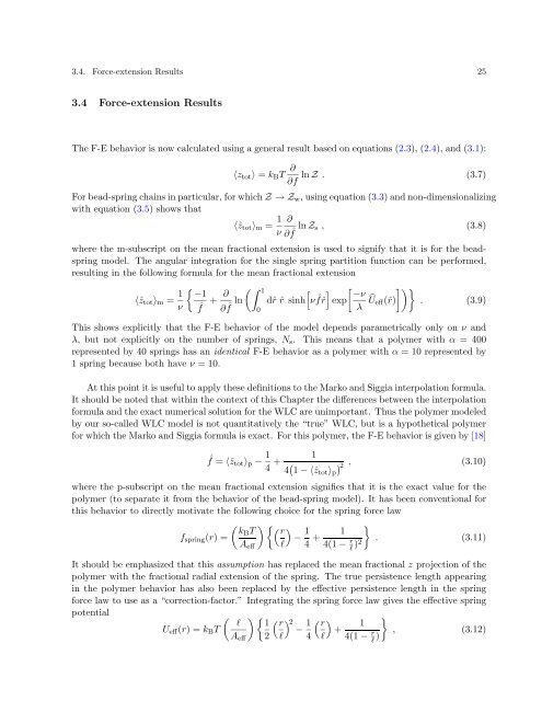
The F-E behavior is now calculated using a general result based on equations (2.3), (2.4), and (3.1):
〈ztot〉 = kBT ∂
ln Z . (3.7)
∂f
For bead-spring chains in particular, for which Z→Zw, using equation (3.3) and non-dimensionalizing
with equation (3.5) shows that
〈ˆztot〉m = 1 ∂
ν ∂ ˆ f ln Zs , (3.8)
where the m-subscript on the mean fractional extension is used to signify that it is for the beadspring
model. The angular integration for the single spring partition function can be performed,
resulting in the following formula for the mean fractional extension
〈ˆztot〉m = 1
−1 ∂
+
ν ˆf ∂ ˆ f ln
1
dˆr ˆr sinh ν
0
ˆ
−ν
f ˆr exp
λ
Ueff(ˆr)
. (3.9)
This shows explicitly that the F-E behavior of the model depends parametrically only on ν and
λ, but not explicitly on the number of springs, Ns. This means that a polymer with α = 400
represented by 40 springs has an identical F-E behavior as a polymer with α = 10 represented by
1 spring because both have ν = 10.
At this point it is useful to apply these definitions to the Marko and Siggia interpolation formula.
It should be noted that within the context of this Chapter the differences between the interpolation
formula and the exact numerical solution for the WLC are unimportant. Thus the polymer modeled
by our so-called WLC model is not quantitatively the “true” WLC, but is a hypothetical polymer
for which the Marko and Siggia formula is exact. For this polymer, the F-E behavior is given by [18]
ˆf = 〈ˆztot〉p − 1
4 +
1
4 2 ,
1 −〈ˆztot〉p
(3.10)
where the p-subscript on the mean fractional extension signifies that it is the exact value for the
polymer (to separate it from the behavior of the bead-spring model). It has been conventional for
this behavior to directly motivate the following choice for the spring force law
kBT
r
fspring(r) =
−
ℓ
1
4 +
. (3.11)
Aeff
1
4(1 − r
ℓ )2
It should be emphasized that this assumption has replaced the mean fractional z projection of the
polymer with the fractional radial extension of the spring. The true persistence length appearing
in the polymer behavior has also been replaced by the effective persistence length in the spring
force law to use as a “correction-factor.” Integrating the spring force law gives the effective spring
potential
ℓ
Ueff(r) =kBT
Aeff
1
2
r
2 −
ℓ
1
4
r
+
ℓ
1
4(1 − r
ℓ )
, (3.12)