Systematic development of coarse-grained polymer models Patrick ...
Systematic development of coarse-grained polymer models Patrick ...
Systematic development of coarse-grained polymer models Patrick ...

Create successful ePaper yourself
Turn your PDF publications into a flip-book with our unique Google optimized e-Paper software.
3.6. Effective Persistence Length 31<br />
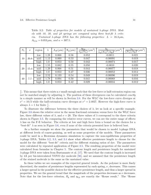
Table 3.2: Table <strong>of</strong> properties for <strong>models</strong> <strong>of</strong> unstained λ-phage DNA. Models<br />
with 10, 20, and 40 springs are compared using three best-fit λ criteria.<br />
Unstained λ-phage DNA has the following properties: L = 16.3 µm,<br />
Atrue =0.053 µm, andα = 307.5.<br />
η0,p<br />
Ns ν region λ Aeff(µm) Rg(µm)<br />
np(Nζ) (µm2 )<br />
b2<br />
np(Nζ) 2 /kBT (µm4 )<br />
τ0<br />
(Nζ)/kBT (µm2 )<br />
low 1.28 0.068 0.56 0.052 -0.0011 0.021<br />
10 30.8 mid 1.13 0.060 0.53 0.047 -0.00091 0.019<br />
high 1.0 0.053 0.50 0.042 -0.00074 0.017<br />
low 1.55 0.082 0.55 0.050 -0.0010 0.020<br />
20 15.4 mid 1.29 0.068 0.51 0.044 -0.00077 0.018<br />
high 1.0 0.053 0.47 0.036 -0.00052 0.014<br />
low 2.52 0.133 0.54 0.049 -0.00096 0.019<br />
40 7.7 mid 1.78 0.094 0.50 0.041 -0.00068 0.016<br />
high 1.0 0.053 0.42 0.029 -0.00034 0.012<br />
1<br />
ν . This means that there exists a ν small enough such that the low-force or half-extension region can<br />
not be matched simply by adjusting λ. The position <strong>of</strong> these divergences can be calculated exactly<br />
in a simple manner as will be shown in Section 3.8. For the WLC the low-force curve diverges at<br />
ν∗ =10/3 while the half-extension curve diverges at ν∗ =2.4827. However the high-force curve is<br />
always λ = 1 for finite 1<br />
ν .<br />
To illustrate the difference between the three choices <strong>of</strong> λ, let us look at a specific example.<br />
Figure 3.6 shows the relative error in the mean fractional extension versus force for the WLC force<br />
law, three different values <strong>of</strong> λ, andν = 20. The three values <strong>of</strong> λ correspond to the three criteria<br />
shown in Figure 3.5. By comparing the relative error curves, we can see the entire range <strong>of</strong> effects<br />
λ has on the F-E behavior. The criteria at low and high force form a bound on the choices for a<br />
“best-fit” λ as seen in Figure 3.6, even if none <strong>of</strong> the criteria presented here is believed best.<br />
As a further example we show the parameters that would be chosen to model λ-phage DNA<br />
at different levels <strong>of</strong> <strong>coarse</strong>-graining, as well as some properties <strong>of</strong> the <strong>models</strong>. These parameters<br />
could be used in a Brownian dynamics simulation to capture the non-equilibrium properties <strong>of</strong><br />
λ-phage DNA. Tables 3.2, 3.3, and3.4 show what effective persistence length to choose for the<br />
model for the different “best-fit” criteria and for different staining ratios <strong>of</strong> dye. The parameters<br />
were calculated by repeated application <strong>of</strong> Figure 3.5. The resulting properties <strong>of</strong> the model were<br />
calculated from formulae in Chapter 5. The contour length and persistence length for unstained<br />
λ-phage DNA were taken from Bustamante et al. [17]. We used that the contour length is increased<br />
by 4˚A per bis-intercalated YOYO dye molecule [56], and we assumed that the persistence length<br />
<strong>of</strong> the stained molecule is the same as the unstained value.<br />
In these tables we see examples <strong>of</strong> the expected general trends. As the <strong>polymer</strong> is more finely<br />
discretized, the number <strong>of</strong> persistence lengths represented by each spring, ν, decreases. This causes<br />
a larger spread in the possible choices for the effective persistence length, and thus a larger spread in<br />
properties. We see the general trend that the magnitude <strong>of</strong> the properties decreases as ν decreases.<br />
Note that for the low-force criterion, Rg and η0,p are exactly the “Rouse result.” The “Rouse