Useful Approximate Solutions for Standard ... - MAELabs UCSD
Useful Approximate Solutions for Standard ... - MAELabs UCSD
Useful Approximate Solutions for Standard ... - MAELabs UCSD

You also want an ePaper? Increase the reach of your titles
YUMPU automatically turns print PDFs into web optimized ePapers that Google loves.
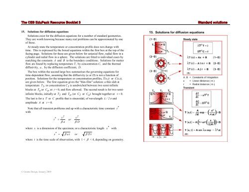
15. <strong>Solutions</strong> <strong>for</strong> diffusion equations<br />
<strong>Solutions</strong> exist <strong>for</strong> the diffusion equations <strong>for</strong> a number of standard geometries.<br />
They are worth knowing because many real problems can be approximated by one<br />
of these.<br />
At steady-state the temperature or concentration profile does not change with<br />
time. This is expressed by the boxed equations within the first box at the top of the<br />
facing page. <strong>Solutions</strong> <strong>for</strong> these are given below <strong>for</strong> uniaxial flow, radial flow in a<br />
cylinder and radial flow in a sphere. The solutions are fitted to individual cases by<br />
matching the constants A and B to the boundary conditions. <strong>Solutions</strong> <strong>for</strong> matter<br />
flow are found by replacing temperature T, by concentration C, and the thermal<br />
diffusivity, a , by the diffusion coefficient, D.<br />
The box within the second large box summarises the governing equations <strong>for</strong><br />
time-dependent flow, assuming that the diffusivity (a or D) is not a function of<br />
position. <strong>Solutions</strong> <strong>for</strong> the temperature or concentration profiles, T(x,t) or C(x,t),<br />
are given below. The first equation gives the "thin-film" solution: a thin slab at<br />
temperature T 1 , or concentration C 1 is sandwiched between two semi-infinite<br />
blocks at T o or C o , at t = 0, and flow allowed. The second result is <strong>for</strong> two semi-<br />
infinite blocks, initially at T 1 and T o , (or C 1 or C o ) brought together at t = 0.<br />
The last is <strong>for</strong> a T or C profile that is sinusoidal, of wavelength λ / 2π<br />
and<br />
amplitude A at t = 0.<br />
Note that all transient problems end up with a characteristic time constant *<br />
t<br />
with<br />
© Granta Design, January 2009<br />
x<br />
2<br />
t<br />
*<br />
=<br />
β a<br />
or<br />
x<br />
2<br />
β D<br />
where x is a dimension of the specimen; or a characteristic length *<br />
x with<br />
x *<br />
=<br />
β a t<br />
or<br />
β D t<br />
where t is the time scale of observation, with 1 < β < 4, depending on geometry.