Astrodynamics 101 - DerAstrodynamics.com
Astrodynamics 101 - DerAstrodynamics.com
Astrodynamics 101 - DerAstrodynamics.com

You also want an ePaper? Increase the reach of your titles
YUMPU automatically turns print PDFs into web optimized ePapers that Google loves.
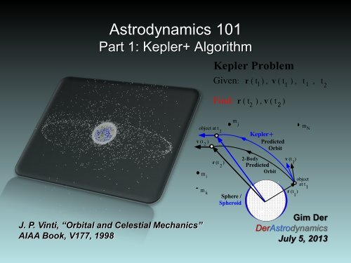
<strong>Astrodynamics</strong> <strong>101</strong><br />
Part 1: Kepler+ Algorithm<br />
J. P. Vinti, “Orbital and Celestial Mechanics”<br />
AIAA Book, V177, 1998<br />
object at t 2<br />
v (t )<br />
2<br />
m i<br />
m<br />
k<br />
Kepler Problem<br />
Given: r ( t ) , v ( t ) , t , t<br />
Find: r ( t ) , v ( t )<br />
r (t )<br />
2<br />
m<br />
j<br />
Sphere /<br />
Spheroid<br />
2<br />
1<br />
+<br />
2<br />
Kepler<br />
Predicted<br />
Orbit<br />
2-Body<br />
Predicted<br />
Orbit<br />
99+%<br />
1<br />
v (t )<br />
1<br />
Gim Der<br />
Der<strong>Astrodynamics</strong><br />
July 5, 2013<br />
1<br />
mN<br />
object<br />
at t<br />
1<br />
r (t )<br />
1<br />
2
Analytic <strong>Astrodynamics</strong> Overview<br />
<strong>Astrodynamics</strong> <strong>101</strong>: Kepler+ Algorithm<br />
Part1: Analytic Prediction Algorithms<br />
Part2: Verifications<br />
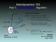
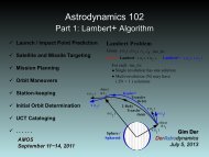
<strong>Astrodynamics</strong> 102: Lambert+ Algorithm<br />
Part1: Analytic Multi-revolution Targeting Algorithms<br />
(Orbit Determination for Radar Data)<br />
Part2: Verifications<br />
<strong>Astrodynamics</strong> 103: Gauss/Laplace+ Algorithm<br />
Part1: Analytic Angles-only Algorithms<br />
(Orbit Determination for Optical Sensor Data)<br />
Part2: Verifications
<strong>Astrodynamics</strong> <strong>101</strong>: Kepler+ Algorithm<br />
Part 1. Analytic Prediction Algorithms<br />
1. What, Why, How<br />
2. Physics<br />
3. Equations of motion<br />
4. Analytic Algorithms for Prediction<br />
5. Applications for SSA<br />
Part 2. Verifications<br />
6. Matter of Reference<br />
7. Numerical Examples
Satellites, Missiles and Debris<br />
Intentional Destruction and Unintentional Space Collisions<br />
2007 2009, . . , 2013<br />
ASAT Test and Space Accidents Happened
Destruction Power of Space Debris<br />
Properties of Space Debris (2010):<br />
Size: Trackable ~ 10 cm (4 in)<br />
speed: > = 10 km/s (+22,000 mph)<br />
Range: 600 to 1600 km (400 to 1000 mi)<br />
Distribution: 7% useful satellites, others junk<br />
The image above shows, the risk of damage is real. This hole over 1 cm (3/8 in)<br />
in diameter penetrates the Hubble high gain antenna dish (the unit continued<br />
working in spite of the damage).<br />
The windows on the Space Shuttles have been replaced 80 times due to<br />
impacts with objects of less than 1 mm (0.04 in). And costly systems to track<br />
and issue daily emails warning of potential impacts must be maintained.
Destruction Power of Space Debris<br />
All it took to punch this 0.025-cm hole in a U.S. satellite was a paint chip moving at hypervelocity<br />
of 9 km/s. When the shuttle brought back the satellite, scientists found six holes per square foot.<br />
(Hole in satellite photograph by NASA.)
How Many? Then (2009)<br />
http://www.ucsusa.org/assets/documents/nwgs/SatelliteCollision-2-12-09.pdf<br />
Size of debris particles 10 cm (4 inches)<br />
(Can be Tracked)<br />
Debris in LEO and HEO<br />
Mostly 600 to 1500 km<br />
14,000<br />
(Space Fence<br />
Targets)<br />
1 cm (0.4 inch)<br />
(Cannot be<br />
Tracked)<br />
370,000<br />
Debris at all altitudes 22,000 750,000<br />
Total estimated debris, by size, in orbit around the earth (26 Feb 2009)
How Many? Now (2013)<br />
http://www.space.<strong>com</strong>/12602-space-junk-cleanup-grand-challenge-21st-century.html<br />
Total estimated debris, by size, in orbit around the earth (8 Mar 2013)
How Debris Clouds Look Like?<br />
Debris clouds after 9 minutes Debris clouds after 10 days<br />
Debris Clouds after 6 months<br />
Debris clouds after 3 years<br />
Debris Generation After a Collision
GS satellite ring<br />
alt. = ~1400 km<br />
rev/day = ~ 12<br />
Conjunction Assessment with Less False Alarms<br />
Real Time and Accurate<br />
Conjunction Assessment<br />
Iridium satellite ring<br />
alt. = ~800 km<br />
rev/day = ~ 14<br />
Less False Alarms
Orbit Determination of All Space Objects for SSA<br />
90% of the Space Objects in Near-Earth<br />
from 22,000 to 100,000 soon<br />
Kepler +, Lambert +, Gauss/Laplace+ Algorithms<br />
Fast and Accurate Analytic <strong>Astrodynamics</strong> Algorithms<br />
for Precise Orbit Determination
1. What, Why, How<br />
What? Cataloging of 100,000+ satellites and<br />
space debris is a challenging Space<br />
Situation Awareness (SSA) problem<br />
Why? Need near real time positions and<br />
characterization of all objects to insure<br />
operation and safety of space assets<br />
How? Understand the Physics and develop<br />
new analytic <strong>Astrodynamics</strong> algorithms<br />
for accurate and fast trajectory prediction<br />
and SSA applications<br />
Building A New Space Catalog of 100,000+ Objects<br />
Requires Analytic Kepler+ Algorithm
object<br />
v (t<br />
2<br />
) at t<br />
2<br />
r (t )<br />
2<br />
Sphere<br />
2-Body<br />
Predicted<br />
Trajectory<br />
r (t )<br />
1<br />
v (t )<br />
1<br />
object<br />
at t 1<br />
Kepler and Kepler+ Algorithms<br />
Kepler Problem<br />
Given: t , t , r ( t ) , v ( t )<br />
1<br />
Find: r ( t ) , v ( t )<br />
2<br />
2<br />
add perturbations analytically<br />
( J 2 , J 3 , J 4 , J 22 , J 31 , . .<br />
Sun , Moon , Drag , . . )<br />
Kepler (2-Body) solution Kepler+ solution for SSA<br />
(accurate and fast )<br />
2<br />
1<br />
1<br />
v (t )<br />
2<br />
Spheroid<br />
object<br />
at t2<br />
r (t )<br />
2<br />
Kepler+<br />
Predicted<br />
Trajectory<br />
r (t )<br />
1<br />
v (t )<br />
1<br />
object<br />
at t 1
Forces and Accelerations<br />
2. Physics
v (t )<br />
object at t<br />
r (t)<br />
Accelerations on Satellite and Rocket (1)<br />
1. Earth spherical gravity (low_g)<br />
2. Earth spheroidal gravity (high_g)<br />
3. Sun gravity<br />
4. Moon gravity<br />
5. Solar radiation pressure<br />
6. Atmospheric (Air) drag<br />
7. Thrust acceleration<br />
Earth<br />
v ( t )<br />
1<br />
object at t<br />
1<br />
r ( t<br />
1<br />
)<br />
Kepler Problem<br />
Given: r (t ) , v (t ) , t , t<br />
1<br />
Find: r (t) , v (t)<br />
1 1
1. Spherical gravity (low_g)<br />
v (t )<br />
object at t<br />
r (t)<br />
<br />
a = r<br />
r 3<br />
low<br />
Example:<br />
MEO / GEO object at t<br />
r = 7,000 / 40,000 km<br />
Accelerations on Satellite and Rocket (2)<br />
Spherical<br />
Earth<br />
a = 8.0 0.2<br />
low<br />
v (t )<br />
m/s 2<br />
2. Spheroidal gravity (high_g)<br />
object at t<br />
r (t)<br />
a = a + a + a + . . +<br />
high<br />
J 2<br />
J 3<br />
J 4<br />
+ a + . . . +<br />
J<br />
22<br />
Oblate Spheroidal<br />
'Flattened' Earth<br />
3<br />
a = 20 x 10 1.0 x 10<br />
high<br />
6<br />
m/s 2
3. Sun gravity<br />
a = r<br />
sun<br />
v (t )<br />
object at t<br />
r (t)<br />
Earth<br />
Accelerations on Satellite and Rocket (3)<br />
Sun<br />
<br />
r (t)<br />
sun<br />
sun<br />
r 3<br />
<br />
a = r<br />
moon<br />
r moon<br />
3<br />
sun moon<br />
v (t )<br />
object at t<br />
r (t)<br />
Earth<br />
Example:<br />
MEO / GEO object at t sun moon<br />
r = 7,000 / 40,000 km m/s 2<br />
6<br />
a = 0.3 x 10<br />
6<br />
2. x 10<br />
4. Moon gravity<br />
r (t)<br />
moon<br />
6<br />
a = 0.6 x 10<br />
5. x 10<br />
Moon<br />
m/s 2 6
5. Solar Radiation Pressure<br />
a (t)<br />
solar<br />
radiation<br />
pressure<br />
v (t )<br />
object at t<br />
r (t)<br />
Earth<br />
Example:<br />
MEO / GEO object at t<br />
r = 7,000 / 40,000 km<br />
Accelerations on Satellite and Rocket (4)<br />
Sun<br />
Photons<br />
r (t)<br />
sun<br />
solar<br />
radiation<br />
pressure<br />
Earth<br />
6<br />
a = 0.1 x 10 m/s 2<br />
Atmo<br />
6. Atmospheric (Air) Drag<br />
sphere<br />
Earth<br />
a = 0<br />
drag<br />
v (t )<br />
r (t)<br />
m/s 2<br />
Earth<br />
Atmosphere<br />
Air<br />
a (t)<br />
drag<br />
effective height<br />
for drag:<br />
Sat. = ~ 200 km<br />
Missile<br />
~<br />
= 60 km<br />
(for short time<br />
prediction)
V<br />
Transfer<br />
Orbit<br />
v<br />
t1<br />
1<br />
v<br />
1<br />
t 1<br />
t<br />
2<br />
r<br />
1<br />
r<br />
2<br />
Earth<br />
v<br />
t2<br />
Accelerations on Satellite and Rocket (5)<br />
Orbit 1<br />
Orbit 2<br />
V<br />
v<br />
2<br />
Satellite Thrusting<br />
(Orbit Change or Maneuver)<br />
2<br />
7. Thrust Accelerations<br />
Lambert Problem<br />
Given: r , r , t , t<br />
1 2 1 2<br />
Find: v (t ) = v , v (t ) =<br />
1<br />
Then <strong>com</strong>pute:<br />
V = v <br />
1<br />
t1<br />
t1<br />
v<br />
1<br />
V = v v<br />
2 2 t2<br />
2<br />
v<br />
t2<br />
Rocket Thrusting<br />
(Ascending from Earth)
7<br />
V<br />
v (t )<br />
object at t<br />
2<br />
4<br />
Protons<br />
r (t)<br />
1<br />
Air<br />
6<br />
Moon<br />
5<br />
Earth<br />
r (t )<br />
1<br />
Accelerations Summary (6)<br />
v (t )<br />
1<br />
object<br />
at t 1<br />
3<br />
Sun<br />
1. Earth low gravity<br />
2. Earth high gravity<br />
3. Sun gravity<br />
4. Moon gravity<br />
5. Proton Pressure<br />
6. Air Drag<br />
7. Thrust Acceleration<br />
Kepler Problem<br />
Given: r (t<br />
1<br />
) , v (t ) , t , t<br />
1 1<br />
Find: r (t) , v (t)<br />
(Pull)<br />
(Pull)<br />
(Pull)<br />
(Pull)<br />
(Push)<br />
(Pull)<br />
(Push)
3. Equations of Motion<br />
Equations<br />
for<br />
Prediction and Propagation
Mathematical Interpretation<br />
<strong>Astrodynamics</strong>: Understanding Forces<br />
Newton’s Formula<br />
General Formula:<br />
Orbiting Satellites:<br />
Missiles / Aircraft:<br />
m<br />
m<br />
m<br />
2<br />
d r d r<br />
= f ( t , r , ) = F<br />
2<br />
d t<br />
d t<br />
2<br />
d r<br />
d t<br />
d t<br />
2<br />
2<br />
d r<br />
r<br />
= f ( ) = F + F<br />
3<br />
gravity<br />
r<br />
others<br />
= F + F + F + F<br />
2 gravity thrust aero wind
Equations<br />
of Motion<br />
Formulation<br />
Who<br />
Analytic<br />
Solution<br />
Force Method<br />
2<br />
d r<br />
dt<br />
2<br />
= <br />
Classical<br />
(Newton)<br />
<br />
Kepler, Newton,<br />
(almost everyone)<br />
Keplerian<br />
(2-body: a d = 0 )<br />
r<br />
3<br />
Comparison of Analytic Methods<br />
r a<br />
d<br />
p<br />
k<br />
H(<br />
q,<br />
p,<br />
t)<br />
,<br />
q<br />
Energy Method<br />
k<br />
Von-Zeipel, Laplace, (Vinti,<br />
(Brouwer, SGP4) Kepler+)<br />
non-Keplerian non-Keplerian<br />
(averaging (general<br />
solution: a<br />
d<br />
0 ) solution: a<br />
d<br />
0 )<br />
q<br />
Hamilton - Jacobi<br />
AIAA book V177, “Orbital and Celestial Mechanics”<br />
k<br />
H(<br />
q,<br />
p,<br />
t)<br />
<br />
p<br />
k
Newton / Classical Formulation<br />
Equations of motion<br />
2<br />
d r <br />
= r a<br />
2 3 d t r<br />
Given : r(t 0), v(t<br />
0), t 0 , t<br />
Find : r(t ) , v(t<br />
)<br />
Kepler method:<br />
Assume zero perturbation:<br />
,<br />
a 0<br />
d =<br />
resulting in spherical<br />
gravity effect.<br />
Kepler analytic solution:<br />
r fI =<br />
v <br />
fI gI<br />
gI<br />
<br />
<br />
r0<br />
v<br />
where f , g, f , and g are<br />
analytic and functions of<br />
r r(t ) and v v(t<br />
)<br />
<br />
<br />
<br />
d<br />
0 <br />
0 0 0 0<br />
UNCLASSIFIED<br />
Comparison of Analytic Solutions<br />
Vinti / Hamilton-Jacobi Formulation<br />
Equations of motion<br />
dpk H(q, p, t ) dqk<br />
H(q,<br />
p, t )<br />
, <br />
d t qk d t pk<br />
where q's and p's are respectively<br />
coordinates and momenta, and k 1,<br />
2, 3<br />
Given : r(t 0), v(t<br />
0), t 0 , t<br />
Find : r(t ) , v(t<br />
)<br />
Vinti method:<br />
Assume non-zero perturbation:<br />
,<br />
a 0<br />
d <br />
resulting in spheroidal gravity effect so that<br />
zonal geopotentials J , J , J are included.<br />
2 3 4<br />
Vinti analytic solution:<br />
See Vinti AIAA book, V177, 1998,<br />
"Orbital and Celestial Mechanics",<br />
Chapter 8.<br />
Also see GTDS, Chapter 5.12 on<br />
attributes of "Vinti Theory", singularity free<br />
and applicability to satellites and missiles.
4. Analytic Algorithms for Prediction<br />
Analytic Algorithms<br />
and<br />
Developement
Analytic Algorithms and Solutions<br />
Important Questions:<br />
1. How accurate? 2. How fast? 3. How robust?<br />
Answers:<br />
1. Accuracy of 10 km to a few centimeters depends<br />
on SSA applications of prediction / tracking /<br />
correlation / conjunction / . . . .<br />
2. Need to process all objects in the current or future<br />
Space Catalog under 12 hours or much quicker<br />
3. Robustness requires algorithms to update everyday<br />
accurately all objects in any Space Catalog of tens<br />
or hundreds of thousands objects
Kepler Equations of Motion (2-Body)<br />
2<br />
d r <br />
= r<br />
2 3 d t r<br />
Kepler Algorithm (2 Steps for solution)<br />
1. Solve Classical or Universal Kepler Eqn<br />
for E or x by an iterative method such as<br />
Newton, Halley or Laguerre<br />
F(E) = E e sinE 0<br />
F (x) = (x) (t 2t 1)<br />
0<br />
2. Compute (t ) and<br />
r(t 2) fI gI<br />
r(t<br />
1)<br />
= <br />
v(t ) fI gI<br />
v(t<br />
)<br />
<br />
<br />
<br />
<br />
<br />
2 1 <br />
where f g<br />
r 2 v 2<br />
(t )<br />
, f g are functions of E or x<br />
, ,<br />
Analytic Kepler Algorithm<br />
Kepler Problem<br />
Given: t , t , r ( t ) , v ( t )<br />
1<br />
Find: r ( t ) , v ( t )<br />
v (t<br />
2<br />
)<br />
r (t )<br />
2<br />
2<br />
object<br />
at t 2<br />
2<br />
2<br />
1<br />
Sphere<br />
Predicted<br />
Trajectory<br />
1<br />
r (t )<br />
1<br />
v (t )<br />
1<br />
object<br />
at t<br />
1
Kepler Problem<br />
Given: r (t 1) , v (t ) , t , t<br />
1 1 2<br />
Find: r (t<br />
2<br />
) , v (t<br />
2<br />
)<br />
v (t<br />
2<br />
) object at t<br />
2<br />
r (t )<br />
2<br />
Exaggerated<br />
Spheroid<br />
>> 1% mass<br />
~ 0.001 m/s**2<br />
acceleration<br />
Vinti<br />
Predicted<br />
Trajectory<br />
v (t )<br />
1<br />
r (t )<br />
1<br />
object<br />
at t 1<br />
Analytic Vinti Algorithm<br />
Vinti Implementation (AIAA Book)<br />
1. Hamilton-Jacobi Equations of motion<br />
2. Transform given ECI state<br />
to Spheroidal coordinates<br />
3. Include J 2 , J 3 , J 4 and solve for<br />
final state in Spheroidal coordinates<br />
4. Transform back to final ECI state<br />
Vinti Theory<br />
(conceptual Equations of motion)<br />
2<br />
d r <br />
= r a a a a<br />
2 3<br />
dt R<br />
Spheroidal<br />
Body<br />
J2 J3 J4 Vinti<br />
Non-Keplerian<br />
(more accurate)<br />
Trajectory
+<br />
Kepler solution<br />
(Vinti and other perturbations)<br />
Numerical accurate<br />
solution (desired)<br />
V (t )<br />
General Equations of motion:<br />
d2<br />
R<br />
= <br />
<br />
R a<br />
2 3 d t R<br />
d<br />
Analytic Kepler+ Algorithm<br />
(3)<br />
Vinti spheroidal<br />
solution only<br />
R (t)<br />
General method of solution<br />
=> Kepler+ solution<br />
(1) Kepler solution only<br />
(2) Kepler + a d perturbed solution<br />
(3) Vinti spheroidal solution only<br />
,<br />
a d =<br />
0<br />
(2) Kepler solution with a<br />
(other perturbations)<br />
Central<br />
Body<br />
(1)<br />
R (t )<br />
1<br />
Kepler<br />
solution only<br />
V (t )<br />
1<br />
object at t 1<br />
d
Vinti and Kepler+ History<br />
Vinti developed theory and algorithm in 1959~1970s<br />
vinti1 – Wadsworth, rocket free-flight, 1963<br />
vinti2 – Izsak-Borchers, ICBM onboard targeting, 1965<br />
vinti3 – Bonavito, Goddard trajectory s/w, 1966<br />
vinti4 – Lang, MIT MS thesis under Vinti, 1968<br />
vinti5 – Getchell, military satellite analysis at NSA, 1970<br />
vinti6 – Der-Monuki, satellite and missile trajectories, 1998<br />
vinti7 – Der, Satellite and Missile trajectories, no singularities, 2009<br />
Kepler+ = Vinti7 + additional perturbations, 2012<br />
Includes analytically additional perturbations of Higher-order<br />
Geopotentials, Sun, Moon, Drag, . . , for Satellites and Missiles<br />
Provides Speed, Robustness and “Near SP” Accuracy needed<br />
for SSA<br />
The most <strong>com</strong>plete General Perturbation algorithms
APL Technical<br />
Digest Vol 27, #3<br />
(2007)<br />
Revisit Key <strong>Astrodynamics</strong> Algorithms<br />
Vinti<br />
Theory (1959)<br />
+ 3 22<br />
rd Kepler+ =<br />
+ J 2 , + J 3 , + J 4 ,<br />
body, J , J 31 ,<br />
drag, . . (2012)<br />
No funding for accurate and<br />
fast analytic <strong>Astrodynamics</strong><br />
algorithms since 1960s!<br />
Spent 50 years funding accurate<br />
but slow <strong>Astrodynamics</strong> algorithms<br />
that are not efficient nor suitable for<br />
SSA<br />
References: SSA papers<br />
• Desrocher,D., “Transforming Space Surveil..”, AAS 05-201<br />
• Morring, F. Jr., “Collision Course”, Aviation Week, March 19, 2012<br />
• Vetter, J.R., “Fifty Years of Orbit Determ . . , APL TD, V27, #3<br />
• . . . . .
Osculating Orbital<br />
Elements at t o<br />
[ r (t ), v (t )]<br />
o o<br />
Radars /<br />
Optical<br />
sensors<br />
Future<br />
look angles<br />
( pointing<br />
prediction )<br />
Others . . . . . .<br />
Orbit Determination and Prediction/Propagation<br />
Object at t<br />
r<br />
Unsuitable for real-time<br />
automatic processing<br />
Ephemerides<br />
(Catalogs)<br />
Raw<br />
Observation<br />
data<br />
v<br />
Orbit<br />
Determination<br />
(Estimated future/past)<br />
position and velocity vectors<br />
Rise/Set<br />
Site visibility<br />
<strong>Astrodynamics</strong><br />
102: Lambert /<br />
103: Gauss/Laplace<br />
Initial Orbit<br />
Determination<br />
Processed<br />
Observation<br />
data<br />
Differential<br />
Correction<br />
Batch / KF<br />
TLE<br />
conversion<br />
difficulties<br />
Singularity<br />
difficulties<br />
Osc2Mean<br />
Analytic algorithms in OD and P/P<br />
need to process 100,000+ Objects<br />
in less than 12 hours with accuracy<br />
of 10 km to centimeters for SSA<br />
(Estimated initial)<br />
positin and<br />
velocity vectors<br />
Orbital<br />
element set<br />
r and v<br />
Prediction /<br />
Propagation<br />
1 2<br />
SP<br />
3<br />
Numerical<br />
SGP4<br />
Integration Kepler+<br />
Close approach<br />
(miss distance)<br />
Osculating Orbital<br />
Elements at t<br />
[ r , v ]<br />
Astro <strong>101</strong>:<br />
Kepler<br />
1<br />
2<br />
3<br />
SGP4 needs TLE<br />
conversion<br />
(not efficient for SSA)<br />
SP is accurate, but<br />
slow for SSA<br />
Kepler+ is accurate<br />
and fast for SSA
Key SSA Features of Kepler+<br />
SGP4 Kepler+<br />
Prediction Speed (~17 / 14+ micro-sec per traj) YES YES<br />
Prediction error growth ( ~5 / 1 km per day) YES YES<br />
Perturbations <strong>com</strong>pliant and analytic YES YES<br />
Same input/output osculating vectors as SP NO YES<br />
Use any initial state vector as SP NO YES<br />
Use new updated state vector and time as SP NO YES<br />
Singularity free for any object or orbit as SP NO YES<br />
Flexibilities for satellite, missile, Earth/Sun, . . NO YES<br />
SP = numerical integration
5. Applications of Analytic Algorithms<br />
SSA Applications
Atm. Drag effects<br />
SS,<br />
ISS<br />
Applications of Analytic Algorithms<br />
Iridium<br />
LEO + MEO<br />
789 – 865 km<br />
Kepler+<br />
to GEO<br />
and<br />
beyond<br />
Cataloged object distribution vs. altitude from LEO to HEO<br />
after the Accidental Collision on February 10, 2009.<br />
Globalstar<br />
Sun & Moon effects
SF<br />
Example: I = J = K = 100<br />
Correlation <strong>com</strong>bination<br />
= I J K = 1,000,000<br />
Takes a few seconds for<br />
a million <strong>com</strong>binations<br />
UNCLASSIFIED<br />
Applications of Analytic Algorithms(2)<br />
Multi-sensor Multi-object UCT Cataloging using Radar Data<br />
Fence or Radar<br />
Correlating<br />
90+ % of<br />
objects to<br />
catalog<br />
SF<br />
J<br />
UCT processing<br />
Solve by New<br />
angles-only algorithm:<br />
3 <strong>com</strong>puted ?<br />
ranges =<br />
I<br />
K<br />
3 detected<br />
ranges
UNCLASSIFIED<br />
Applications of Analytic Algorithms(3)<br />
Multi-sensor Multi-object UCT Cataloging using Optical Sensor Data
Problem: SSA<br />
Applications of Analytic Algorithms(4)<br />
Solution: Analytic <strong>Astrodynamics</strong>
Analytic Algorithm Pioneer -- Prof. Brouwer<br />
Professor Dirk Brouwer lecturing on the motion of the Moon
Analytic Algorithm Pioneer -- Prof. Vinti<br />
Professor John Vinti lecturing on Potential Theory
<strong>Astrodynamics</strong> <strong>101</strong><br />
Part 2: Verifications of Prediction Algorithms<br />
Space Situation Awareness (SSA)<br />
Uncorrelated Target (UCT) Cataloging<br />
Satellite and Debris Conjunction<br />
and Collision<br />
Satellite and Missile Prediction<br />
and Propagation<br />
Orbit Determination<br />
. . .<br />
J. P. Vinti, “Orbital and Celestial Mechanics”<br />
AIAA Book, V177, 1998<br />
Gim Der<br />
Der<strong>Astrodynamics</strong>
<strong>Astrodynamics</strong> <strong>101</strong><br />
Part 2: Verifications for SSA<br />
(Also please download iOrbit:<br />
http://derastrodynamics.<strong>com</strong>/index.php?main_page=index&cPath=1_7<br />
and run kep for <strong>Astrodynamics</strong> <strong>101</strong> Verifications)<br />
Next
Reference Trajectory (General)<br />
6. Matter of Reference<br />
• Numerical integration with perturbations (Slide 15 to 21)<br />
gives analytic solutions with kilometer accuracy<br />
• Numerical integration with additional perturbations<br />
(time and coordinate, tides, J [C and S ], planets, . . . , )<br />
gives numerical solutions with centimeter (or less) accuracy<br />
Reference Trajectory (Section 7. Numerical Examples)<br />
• Numerical integration with perturbations<br />
(WGS84 12x12, Sun, Moon, Drag)<br />
21 21 21<br />
Comparison (Algorithms and Criteria)<br />
• Kepler, SGP4, Vinti, Kepler+, numerical integration with<br />
perturbations (WGS84 4x4, Sun, Moon, Drag)<br />
• CPU timing, accuracy, robustness, mean, standard deviation, max
UNCLASSIFIED<br />
7. Numerical Examples<br />
Numerical Examples<br />
of<br />
Geocentric Objects
Numerical Example 1<br />
Kepler_Test1 * (Analytic Kepler algorithms <strong>com</strong>pared with Numerical Integration)<br />
High Earth Orbit (HEO) , typical 2-Body solutions using the 2007 TLE file<br />
Input: (2007_249, isat = 28836)<br />
t1 = 0., t2 = 86400. (seconds)<br />
Output: kepler1a failed to converge, kepler1b and kepler2 converged to correct answer<br />
algorithms r_eci (t2) (km) v_eci (t2) (km/s)<br />
kepler1a 53052.0539 54034.8022 30994.6668<br />
kepler1b 27456.2663 16961.1113 15098.0763<br />
kepler2 27456.2663 16961.1113 15098.0763<br />
Num. Int.<br />
(2-Body)<br />
r_eci (t1) (km) v_eci (t1) (km/s)<br />
2218.922362 13049.809380 15.285102 3.894738598 4.630875574 2.332314347<br />
*<br />
27456.2662 16961.1114 15098.0764<br />
6.451059 4.143735 2.850977<br />
1.431551 1.341058 0.596545<br />
1.431551 1.341058 0.596545<br />
1.431551 1.341058 0.596545<br />
Free download: Kepler_Test <strong>com</strong>puter programs with source code
Numerical Example 2<br />
Kepler_Test1 * (Analytic Kepler algorithms <strong>com</strong>pared with Numerical Integration)<br />
High Earth Orbit (HEO) , typical 2-Body solutions using the 2009 TLE file<br />
Input: (2009_298, isat = 19773)<br />
t1 = 0., t2 = 86400. (seconds)<br />
Output: kepler1b failed to converge, kepler1a and kepler2 converged to correct answer<br />
DerAstro r_eci (t2) (km) v_eci (t2) (km/s)<br />
kepler1a 16906.0049 1871.5115 2495.6926 4.125426 3.558097 0.604363<br />
kepler1b 99927.4767 92921.1426 14631.3162 5.642214 7.607469 0.840981<br />
kepler2 16906.0049 1871.5115 2495.6926 4.125426 3.558097 0.604363<br />
Num. Int.<br />
(2-Body)<br />
r_eci (t1) (km) v_eci (t1) (km/s)<br />
209.011468 30385.859968 4.280644 2.248716032 2.177749649 0.329155365<br />
*<br />
16906.0051 1871.5115 2495.6927 4.125426 3.558097 0.604363<br />
Free download: Kepler_Test <strong>com</strong>puter programs with source code
Numerical Example 3<br />
Analytic Kepler, SGP4, Vinti, Kepler+ algorithms and num. int. (wgs 4x4, . . .)<br />
<strong>com</strong>pared with num. int. (wgs 12x12, . . .)<br />
Low Earth Orbit (LEO) , typical 2-Body and perturbed solutions using the 2009 TLE file<br />
Input: (2009_249, isat = 4382)<br />
t1 = 0., t2 = 86400. (seconds)<br />
Algorithm r_eci (t2) (km) v_eci (t2) (km/s)<br />
kepler2 346.687092 6795.012489 412.914501<br />
sgp4 257.913989 6719.684754 1214.516634<br />
vinti 207.380964 6701.510662 1337.255798<br />
kepler+ 213.326456 6703.763322 1322.957867<br />
num. int.<br />
(4x4, . .)<br />
num. int.<br />
(12x12, . .)<br />
r_eci (t1) (km) v_eci (t1) (km/s)<br />
510.306735 6793.878710 0.007287 2.949065600 0.256823630 7.486987267<br />
Output: kepler2 is poor. sgp4 is fair. vinti is reasonable.<br />
kepler+ and num. int. (4x4, . .) produced good solutions for SSA purposes.<br />
213.622528 6703.908820 1322.028866<br />
216.109788 6704.762171 1316.193868<br />
2.978862 0.215630 7.472634<br />
3.040136 1.016065 7.361291<br />
3.045054 1.156390 7.334489<br />
3.044552 1.140038 7.337720<br />
3.044515 1.139009 7.337933<br />
3.044353 1.132308 7.339295
Numerical Example 4<br />
Analytic Kepler, SGP4, Vinti, Kepler+ algorithms and num. int. (4x4, . . .)<br />
<strong>com</strong>pared with num. int. (12x12, . . .)<br />
Low Earth Orbit (LEO) , typical 2-Body and perturbed solutions using the 2009 TLE file<br />
Input: (2009_249, isat = 23282)<br />
t1 = 0., t2 = 86400. (seconds)<br />
Algorithm r_eci (t2) (km) v_eci (t2) (km/s)<br />
kepler2 5496.729940 3059.667485 3715.519008<br />
sgp4 5233.338371 2920.278629 4171.411336<br />
vinti 5240.654526 2919.268575 4163.061193<br />
kepler+ 5248.036696 2918.287891 4154.564282<br />
num. int.<br />
(4x4, . .)<br />
num. int.<br />
(12x12, . .)<br />
r_eci (t1) (km) v_eci (t1) (km/s)<br />
6969.687412 2195.624199 0.030412 0.695626778 2.267918155 6.958092777<br />
Output: kepler2 is poor. sgp4 is fair. vinti is reasonable.<br />
kepler+ and num. int. (4x4, . .) produced good solutions for SSA purposes.<br />
5248.183301 2918.362041 4154.359585<br />
5250.523888 2917.968463 4151.680633<br />
4.385493 0.712399 5.858270<br />
4.806832 0.629942 5.529725<br />
4.798649 0.634552 5.536259<br />
4.790380 0.639186 5.542832<br />
4.790136 0.639259 5.543012<br />
4.787513 0.640780 5.545121
Algorithm<br />
SGP4<br />
(analytic)<br />
Vinti<br />
(analytic)<br />
Kepler+<br />
(analytic)<br />
Numerical<br />
Integration<br />
(4x4, 200s)<br />
Comparison of CPU timing, Perturbations, Singularity<br />
2007 (Sep 6)<br />
11140 objects<br />
CPU timing (micro-seconds)<br />
per trajectory<br />
18.2<br />
14.0<br />
8,400.<br />
127,000.<br />
2009 (Oct25)<br />
14327 objects<br />
17.4<br />
14.2<br />
8,000.<br />
127,000.<br />
2011 (Jan 5)<br />
14638 objects<br />
17.4<br />
13.9<br />
7,800.<br />
127,000.<br />
Perturbations<br />
J 2 , J 3 , J 4<br />
Sun, Moon, Drag<br />
J 2 , J 3 , J 4<br />
J 2 , J 3 , J 4 ,<br />
J 22 , J 31,<br />
J 32 , 33<br />
J ,<br />
Sun, Moon, Drag<br />
WGS84 4x4<br />
Sun, Moon, Drag<br />
Singularity<br />
Yes<br />
No<br />
No<br />
No
Algorithm<br />
(Reference =<br />
WGS84 12x12,<br />
Sun, Moon,<br />
Drag)<br />
SGP4<br />
(analytic)<br />
Vinti<br />
(analytic)<br />
Kepler+<br />
(analytic)<br />
Numerical<br />
Integration<br />
(4x4, 200s)<br />
Comparison of Robustness, Mean and Standard Deviation<br />
2007<br />
total # of objs = 11140<br />
# of objects<br />
with position mean<br />
difference / std (km)<br />
> 5 km<br />
7043<br />
4129<br />
1117<br />
131<br />
Robustness, mean and standard deviation (std)<br />
for one day prediction<br />
53. / 421.<br />
5.3 / 5.0<br />
2.3 / 1.9<br />
1.5 / 1.4<br />
2009<br />
total # of objs = 14327<br />
# of objects<br />
with position mean<br />
difference / std (km)<br />
> 5 km<br />
9028<br />
5399<br />
1964<br />
216<br />
52. / 257.<br />
5.4 / 5.1<br />
2.6 / 2.1<br />
1.7 / 1.4<br />
2011<br />
total # of objs = 14638<br />
# of objects<br />
with position mean<br />
difference / std (km)<br />
> 5 km<br />
9289<br />
5453<br />
1896<br />
177<br />
46. / 195.<br />
5.5 / 5.3<br />
2.6 / 2.0<br />
1.6 / 1.4
Algorithm<br />
(Reference =<br />
WGS84 12x12,<br />
Sun, Moon,<br />
Drag)<br />
SGP4<br />
(analytic)<br />
Vinti<br />
(analytic)<br />
Kepler+<br />
(analytic)<br />
Numerical<br />
Integration<br />
(4x4, 200s)<br />
Comparison of Robustness and Max Error wrt Reference<br />
Robustness and max error with respect to Reference<br />
for one day prediction<br />
2007<br />
total # of objs = 11140<br />
# of objects<br />
with position max error<br />
difference (km)<br />
> 10 km<br />
4767<br />
2093<br />
25<br />
7<br />
37828.<br />
84.<br />
32.<br />
20.<br />
2009<br />
total # of objs = 14327<br />
# of objects<br />
with position max error<br />
difference (km)<br />
> 10 km<br />
6243<br />
2727<br />
39<br />
11<br />
13138.<br />
128.<br />
38.<br />
25.<br />
2011<br />
total # of objs = 14638<br />
# of objects<br />
with position max error<br />
difference (km)<br />
> 10 km<br />
6161<br />
2912<br />
32<br />
6<br />
6025.<br />
73.<br />
31.<br />
15.
UNCLASSIFIED<br />
7. Numerical Examples<br />
Numerical Examples<br />
Of<br />
Geocentric Objects<br />
(More examples available upon request)
UNCLASSIFIED<br />
7. Numerical Examples<br />
Numerical Examples<br />
Of<br />
Heliocentric Objects<br />
(Available upon request, but Not for SSA)