Astrodynamics 102 - DerAstrodynamics.com

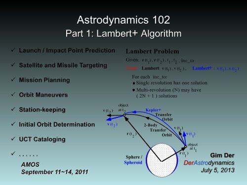
Launch / Impact Point Prediction
Satellite and Missile Targeting
Mission Planning
Orbit Maneuvers
Station-keeping
Initial Orbit Determination
UCT Cataloging
. . . . . .
AMOS
September 11~14, 2011
Astrodynamics 102
Part 1: Lambert+ Algorithm
v (t )
2
v (t )
2
object
at t 2
Lambert Problem
Given: r (t ) , r (t ) , t , t
1 2 1 2 , inc_to
Find:
Lambert: v (t ) , v (t ) , Lambert : v (t ) , v (t )
r (t )
2
1
For each inc_to:
Single revolution has one solution
Multi-revolution (N) may have
( 2N + 1 ) solutions
Sphere /
Spheroid
Kepler+
Transfer
Orbit
2-Body
Transfer
Orbit
2
v (t )
1
r (t )
1
v (t )
1
object
at t
1
+
1 2
Gim Der
DerAstrodynamics
July 5, 2013

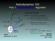
Analytic Astrodynamics Overview
Astrodynamics 101: Kepler+ Algorithm
Part1: Analytic Prediction Algorithms
Part2: Verifications
Astrodynamics 102: Lambert+ Algorithm
Part1: Analytic Multi-revolution Targeting Algorithms
(Orbit Determination for Radar Data)
Part2: Verifications
Astrodynamics 103: Gauss/Laplace+ Algorithm
Part1: Analytic Angles-only Algorithms
(Orbit Determination for Optical Sensor Data)
Part2: Verifications

Astrodynamics 102: Lambert+ Algorithm
Part 1. Analytic Multi-rev Targeting Algorithms
1. What, Why, How
2. Physics and Mathematics
3. Lambert Algorithm Implementation
4. Analytic Lambert Solutions
5. Applications for SSA
Part 2. Verifications
6. Matter of Reference
7. Numerical Examples

2007
Satellites Rendezvous and Docking
Space Shuttle Discovery and ISS
Chinese Spacecraft and CSS

Radar/Laser Weather/Satellite Tracking
Radar
Beam
Weather
forecast
by Radar
Satellite
tracking
by Radar
Satellite
tracking
by Laser
Laser
Beam

Radar Missile Tracking
2007 2009, . . , 2013

Space Debris Collisions
2007 2009, . . , 2013

Space Debris and Satellite Growth
2007 2009, . . , 2013

1. What, Why, How
What? Satellite rendezvous and docking, weather
forecast, tracking of satellites, missiles
and debris, mission planning, . . . . . , SSA
are many challenging problems
Why? Need accurate, fast and robust utility
algorithms for multiple applications
How? Understand the Physics and Mathematics
of Astrodynamics for analytic orbit
determination using radar and laser data
Solving These Challenging Problems
Requires Analytic Lambert+ Algorithm

v (t )
2
object
at t 2
r (t )
2
Sphere
2-Body
Transfer
Orbit
Lambert and Lambert+ Algorithms
Lambert Problem
Given: r (t ) , r (t
2
) , t , t
1
1 2 , inc_to
Find: Lambert: v (t ) , v (t ) ,
v (t )
1
r (t )
1
object
at t
1
1
For each inc_to:
Single revolution has one solution
Multi-revolution (N) may have
( 2N + 1 ) solutions
2
Lambert + : v (t
1
) , v (t 2 )
r (t )
2
Lambert (2-Body) solution Lambert+ solution for SSA
(accurate and fast )
v (t )
2
object
at t 2
add perturbations analytically
( J 2 , J 3 , J 4 , J 22 , J 31 , . .
Sun , Moon , Drag , . . )
Spheroid
Kepler+
2-Body
Transfer
Orbit
v (t )
1
r (t )
1
object
at t
1

Physics and Mathematics
2. Physics

Five SSA Features of Lambert+
Classical Lambert+
Lambert
Inclination indication of transfer orbit,
inc_to, specified NO/maybe YES
Bounded independent variable NO/maybe YES
Robust multi-revolution capability NO/maybe YES
Accurate iterative method YES YES
Perturbations compliant and analytic NO YES

direct transfer orbit
o
(inclination 90 )
r 2
k = (0, 0, 1)
o
r 1
in-plane
h = r x r 1 2
r
2 = k h r
2
h = r x r 1 2
= k h
= < o
= 2
= <
o
= 2
o
Inclination indication
of transfer orbit,
inc_to = 1, posigrade
= 1, retrograde
1
= cos<
r r2 o
[ ]
r r 2
1
r 1
in-plane
Choice of additional input
for Lambert problem:
Inclination
Indication of
Transfer orbit,
Inc_to
(Escobal)
Better for
multi-rev
vs.
transfer
method
or transfer
motion
direction
(Others)

Solution is
guaranteed
Bounded Independent Variable
Bounded x Unbounded x
0 solution
x
Good choice of independent variable:
1. x is bounded
2. Slope d/dx is fit for many
iterative methods
non-dimensional
transfer time
= o is given
o 2 solutions
o 1 solution
Poor choice of independent variable:
1. x is unbounded
2. Slope d/dx is unfit for most
iterative method
Uncertainties in:
1. Initial guess of x
2. Convergence
2 solutions?
Slope
(d/dx)
x

Choice of bounded x, gives a
“vertical U”, allowing A be found easily.
Then with 0
given, the number of
solutions, 0, 1, or 2 can be determined.
Robust Multi-revolution Capability
Multi-revolution, N > 0, needs to determine the minimum time point, A
Bounded Unbounded
x
Vertical U
o
(If x is the “path
parameter”, then
it is bounded)
= o is given
2 solutions
x
N > 0
1 solution
A A ?
0 solution
x
-1 0 +1
0
o
# of solutions?
N > 0
(If x is the semi-
major axis, then
it is unbounded)
Horizontal U
Wrong choice of x leads
to difficulties of finding A,
on a “horizontal U”
flat curve
x

Vary n = 2, 3, . . . , as needed
Solve
with
Accurate Laguerre Iterative Method
where , , are known, and
A micro-second slower, but convergence assured

Classical Kepler
(2-Body)
Perturbations Compliant Analytic Lambert+
Classical Lambert
(2-Body)
Astrodynamics 101
Vinti
(J2, J3, J4
included)
Astrodynamics 102
+ Targeting
by Kepler+
Kepler+
(J2, J3, J4
and other
perturbations))
Lambert+
(J2, J3, J4
and other
perturbations))

3. Analytic Lambert Algorithms
Lambert Algorithmic
Implementations

Equations of Motion (2-Body)
d2
r
=
r
d t2 r3
Lambert Algorithm
1. Classical and Universal Lambert Equations
2. Implementation by Laguerre Iterative Equation
n F (x i )
i+1 i
for i 1,
2, ..
F (x i ) 2 2
F (x i ) (n 1) F (x i ) n (n 1)
F (x i )F (x i )
F (x i )
x x
3
F (a ) = a [( sin ) sin )] t 0
F ( x ) = ( x ) y ) 0
Classical Lambert Algorithm
(single revolution)
(fixed n)
Lambert Problem
Given: r (t ) , r (t ) , t , t , inc_to
Find: v (t ) , v (t )
1
1
v (t
2
) object at t
2
r (t )
2
2
2
1 2
Note:
inc_to given: one solution
if not given: two solutions
2-Body
Transfer
Orbit
Spherical
Earth
v (t )
1
object at t
1
r (t )
1

2-Body Lambert Algorithm
Lambert's Equation for multi-revolutions (Sun)
F ( x) = (x ) y) N 0
Iterative Equation (Laguerre)
Multi-revolution Lambert Algorithm
n F (x i )
i+1 i
for i 1,
2,..
F (x i ) 2 2
F (x i ) (n 1) F (x i ) n (n 1)
F (x i )F (x i )
F (x i )
x x
References:
Sun, F.T., “On The Minimum Time Traj . . ”, AAS 79-164
Der, G. J., “The Superior Lambert Algorithm”, AMOS,2011
v (t )
Lambert Problem
Given: r (t ) , r (t ) , t , t , inc_to
Find: v (t ) , v (t )
object at t 2
2
Transfer
Orbit 2
1
r (t )
2
1
v (t )
2
2
2
Transfer
Orbit 1
Sphere
1 2
Transfer orbit 1: inc_to = 1, i < 90 o
Transfer orbit 2: inc_to = 1, i > 90 o
Multi- revolutions (N)
may have ( 2N + 1 ) solutions
for each inc_to and a given
v (t )
1
r (t )
1
object at t 1
v (t )
1

v 2
vv2 vt2 v 2
Initial
Step 1 B Kepler
r
2
A
Lambert
C
Step 2
A
r
2
C
v 2
Targeting by
Kepler + at t2
Final
Kepler
i
+
+
Final position at t
2
A
k
Targeting to Lambert+
Celestial Pole
Central
body
Final Kepler
trajectory
Given: r , r , t = t t , Computed v , v (Lambert)
1 2 2 1
t1 t2
Find: v , v (Lambert )
v1 v2
r 2
+
Lambert
trajectory
r
1
j
v 1
v 1
+
v 1
v t1
v v1
Initial
position at t
1

4. Analytic Lambert Solutions
Lambert Solutions
and
Orbit Determination

Transfer orbit 1: inc_to = 1, i < 90 o
Transfer orbit 2: inc_to = 1, i > 90 o
v (t )
Single revolution has one solution
for each inc_to and a given
0 < < , 0 < < 1
object at t 2
2
Transfer
Orbit 2
r (t )
2
v (t )
2
Transfer
Orbit 1
v (t )
1
r (t )
1
Sun, F.T., AAS Paper 79-164,
“On the minimum time trajectory and
multiple solutions of Lambert problem”
Sphere
Single Revolution Lambert Solutions
object at t 1
v (t )
1
( Given time difference )
1/ 2
Normalized Time
tm ]
3
3
High Path Low Path
Elliptic Orbits
Path parameter,
1 < x < 1
ME Path line
N = 0
o
( Single revolution, N = 0, 0 < < 360 )
( Unknown to be solved for )
Parabolic Orbits
Path parameter, x = 1
Hyperbolic Orbits
Path parameter, x > 1
ME: Minimum Energy
x

Transfer orbit 1: inc_to = 1, i < 90 o
Transfer orbit 2: inc_to = 1, i > 90 o
v (t )
Multi- revolutions (N)
may have ( 2N + 1 ) solutions
for each inc_to and a given
object at t 2
2
Transfer
Orbit 2
0 < < , 0 < < 1
r (t )
2
v (t )
2
Transfer
Orbit 1
Sun, F.T., AAS Paper 79-164,
“On the minimum time trajectory and
multiple solutions of Lambert problem”
Sphere
v (t )
1
r (t )
1
Multi- Revolution Lambert Solutions
object at t 1
v (t )
1
( Given time difference )
1/ 2
Normalized Time
tm ]
3
3
High Path Low Path
ME Path line
N = 2
N = 1
N = 0
Elliptic Orbits
Path parameter,
1 < x < 1
( x = Unknown to be solved for )
N = Revolution number
( Multi revolution, N > 0, > 360 )
Parabolic Orbits
Path parameter, x = 1
Hyperbolic Orbits
Path parameter, x > 1
ME: Minimum Energy
x
o

Lambert Problem
Given: r (t ) , r (t ) , t , t , inc_to
Find: v (t ) , v (t )
1
Spherical
Earth
1
2
2
1 2
Good: 2-Body Lambert solution
Spheroidal
Earth
2-Body/Keplerian
Trajectory
Better: Targeting by Kepler+
Lambert+ solution
2-Body vs. Lambert+ Solutions
Kepler+ Trajectory
_
(J 2 , J 3 , J 4 + N Body ,
+ J , J , Drag , . .)
31 32
2-Body
v (t
2
)
Lambert+
object
at t 2
r (t )
2
Sphere /
Spheroid
Kepler+
Transfer
Orbit
2-Body
Transfer
Orbit
2-Body Lambert+
v (t )
1
r (t )
1
object
at t
1

Two Equations
and
Two Unknowns
Gauss
Battin
Shepperd
Gooding
Klumpp
Theories/
Formulations
Lambert Algorithm Developers
One Equation
and
One Unknown
Lambert
Gauss
Battin
Lancaster/Blanchard
Godal
Vinh
Sun
Lambert Algorithm Characteristics:
Implementations/
Iterative Methods
Newton,
Halley,
and Others
Everyone
(almost)
Laguerre
and Modified
Laguerre
Conway
Der
1. Most (over 90%) Lambert algorithms apply to zero rev and have singularities
2. Sun/Der Lambert + algorithm applies to multi-rev and rarely has singluarity
(simple theory + straightforward implementation = speed, accuracy, robustness)

Osculating Orbital
Elements at t o
[ r (t ), v (t )]
o o
Radars /
Optical
sensors
Future
look angles
( pointing
prediction )
Others . . . . . .
Orbit Determination and Prediction/Propagation
Object at t
r
Unsuitable for real-time
automatic processing
Ephemerides
Raw
Observation
data
v
Orbit
Determination
(Estimated future/past)
position and velocity vectors
Rise/Set
Site visibility
Astrodynamics
102: Lambert /
103: Gauss/Laplace
Initial Orbit
Determination
Processed
Observation
data
Differential
Correction
Batch / KF
TLE
conversion
difficulties
Singularity
difficulties
Osc2Mean
Analytic algorithms in OD and P/P
need to process 100,000+ Objects
in less than 12 hours with accuracy
of 10 km to centimeters for SSA
(Estimated initial)
positin and
velocity vectors
Orbital
element set
r and v
Prediction /
Propagation
1 2
SP
3
Numerical
SGP4
Integration Kepler+
Close approach
(miss distance)
[ r , v ]
Astro 101:
Kepler
1
2
3
SGP4 needs TLE
conversion
(not efficient for SSA)
SP is accurate, but
slow for SSA
Kepler+ is accurate
and fast for SSA

SSA and Other
Applications
5. Applications

Applications of Analytic Algorithms(1)
Missile Launch- and impact-Point Predictions
A Few Minutes Too Late for any Intercept
BM – Impact Point
Predictions
• Numerical solutions
possible but too late
for countermeasures
• Analytic Lambert+
(speed & accuracy)

SF
Example: I = J = K = 100
Correlation combination
= I J K = 1,000,000
UNCLASSIFIED
Applications of Analytic Algorithms(2)
Multi-sensor Multi-object UCT Cataloging using Radar Data
Fence or Radar
Correlating
90+ % of
objects to
catalog
Takes a few seconds for
a million combinations
SF
J
UCT processing
Solve by New
angles-only algorithm:
3 computed ?
ranges =
I
K
3 detected
ranges

UNCLASSIFIED
Applications of Analytic Algorithms(3)
Multi-sensor Multi-object UCT Cataloging using Optical Sensor Data

Problem: SSA
Applications of Analytic Algorithms(4)
Solution: New Analytic Astrodynamics algorithms

Astrodynamics 102
Part 2: Verifications
(Please download iOrbit:
http://derastrodynamics.com/index.php?main_page=index&cPath=1_7
and run lam for Astrodynamics 102 Verifications)
Next

ICBM transfer orbit , Single revolution 2-Body solution
Input:
Numerical Example 1
inc_to = 1, (inclination of transfer orbit < 90 deg.), t1 = 0., t2 = 1618.50 (seconds)
Output: lambert2 converged to the correct 2-Body solution
*
r_eci (t1) (km) r_eci (t2) (km)
computed inclination of transfer orbit = 67.895 deg., transfer angle = 296.368 deg.
Rev # Path, x v_eci (t1) (km/s) v_eci (t2) (km/s)
N = 0
*

ICBM transfer orbit , Single revolution 2-Body solution
Input:
Output: lambert2 converged to the correct 2-Body solution
Numerical Example 2
inc_to = 1, (inclination of transfer orbit > 90 deg.), t1 = 0., t2 = 1618.50 (seconds)
*
r_eci (t1) (km) r_eci (t2) (km)
computed inclination of transfer orbit = 112.105 deg., transfer angle = 63.632 deg.
Rev # Path, x v_eci (t1) (km/s) v_eci (t2) (km/s)
*
N = 0

Numerical Example 3
High Earth Orbit (Molniya transfer orbit) , Multi- revolution 2-Body solutions
Input:
inc_to = 1, (inclination of transfer orbit < 90 deg.), t1 = 0., t2 = 36000. (seconds)
Output: lambert2 converged to correct 2-Body solutions
*
* inc_to as input dictates the inclination of the transfer orbit.
r_eci (t1) (km) r_eci (t2) (km)
computed inclination of the three transfer orbits = 63.388 deg., transfer angle = 44.705 deg.
Rev # Path, x v_eci (t1) (km/s) v_eci (t2) (km/s)
N = 0
N = 1
N = 1
*
Also allows multi-rev solutions better grouping, as all solutions (N = 0, 1) have the same inclination
and transfer angle.

Numerical Example 4
High Earth Orbit (Molniya transfer orbit) , Multi- revolution 2-Body solutions
Input:
inc_to = 1, (inclination of transfer orbit > 90 deg.), t1 = 0., t2 = 36000. (seconds)
Output: lambert2 converged to correct 2-Body solutions
* computed inclination of the three transfer orbits = 116.612 deg., transfer angle = 315.295 deg.
* inc_to as input dictates the inclination of the transfer orbit.
r_eci (t1) (km) r_eci (t2) (km)
Rev # Path, x v_eci (t1) (km/s) v_eci (t2) (km/s)
N = 0
N = 1
N = 1
*
Also allows multi-rev solutions better grouping, as all solutions (N = 0, 1) have the same inclination
and transfer angle.

Numerical Example 5
ICBM transfer orbit , Single revolution 2-Body, Vinti targeting, Kepler+ targeting solutions
Input:
clock1 = at t1 (needed for Lambert+)
inc_to = 1, (inclination of transfer orbit < 90 deg.), t1 = 0., t2 = 1618.50 (seconds)
Output:
* computed inclination of transfer orbit = 67.895 deg., transfer angle = 296.368 deg.
Algs. Rev# v_eci (t1) (km/s) v_eci (t2) (km/s)
2-Body N =0
Vinti
_targeting
r_eci (t1) (km) r_eci (t2) (km)
N = 0
Lambert+ N = 0
*

Numerical Example 6
ICBM transfer orbit , Single revolution 2-Body, Vinti targeting, Kepler+ targeting solutions
Input:
clock1 = at t1 (needed for Lambert+)
inc_to = 1, (inclination of transfer orbit > 90 deg.), t1 = 0., t2 = 1618.50 (seconds)
Output:
*
Algs. Rev# v_eci (t1) (km/s) v_eci (t2) (km/s)
2-Body N = 0
Vinti
_targeting
r_eci (t1) (km) r_eci (t2) (km)
computed inclination of transfer orbit = 112.105 deg., transfer angle = 63.632 deg.
N = 0
Lambert+ N = 0
*

Numerical Example 7
Molniya transfer orbit , Multi- revolution 2-Body, Vinti targeting, Kepler+ targeting solutions
Input:
clock1 = at t1 (needed for Lambert+)
inc_to = 1, (inclination of transfer orbit < 90 deg.), t1 = 0., t2 = 36000. (seconds)
Output:
r_eci (t1) (km) r_eci (t2) (km)
computed inclination of the three transfer orbits = 63.388 deg., transfer angle = 44.705 deg.
Algs. Rev# v_eci (t1) (km/s) v_eci (t2) (km/s)
2-Body, N = 0
Vinti_targ N = 0
Lambert+ N = 0
2-Body, N = 1
Vinti_targ N = 1
Lambert+ N = 1
2-Body, N = 1
Vinti_targ N = 1
Lambert+ N = 1

Numerical Example 8
Molniya transfer orbit , Multi- revolution 2-Body, Vinti targeting, Kepler+ targeting solutions
Input:
clock1 = at t1 (needed for Lambert+)
inc_to = -1, (inclination of transfer orbit > 90 deg.), t1 = 0., t2 = 36000. (seconds)
Output:
r_eci (t1) (km) r_eci (t2) (km)
computed inclination of the three transfer orbits = 116.612 deg., transfer angle = 315.295 deg.
Algs. Rev# v_eci (t1) (km/s) v_eci (t2) (km/s)
2-Body, N = 0
Vinti_targ N = 0
Lambert+ N = 0
2-Body, N = 1
Vinti_targ N = 1
Lambert+ N = 1
2-Body, N = 1
Vinti_targ N = 1
Lambert+ N = 1

Lambert+ Verifications
Astrodynamics 102
Part 2: Verifications
(Please download iOrbit:
http://derastrodynamics.com/index.php?main_page=index&cPath=1_7
and run lam for Astrodynamics 102
for more Lambert+ Verifications)