Problem Set 1 Introduction to Geological Oceanography Winter ...

Problem Set 1
Introduction to Geological Oceanography Winter 2010
due Thursday Jan 28. All questions are worth 20 pts (grad students) or 25 pts (undergrads).
1. Fig. 1a shows representative travel-time curves for a number of different seismic rays. Draw a
cross-section of the earth, separate it into its major seismic discontinuities and draw examples of the
following ray paths (P, S, PP, SS, PPP, SSS, PcP, ScS, PcS, PKP, SKS, PKIKP.
Use the travel-time curves to determine the distance away from the source that the earthquake shown
in fig 1b is recorded assuming that it occurred near the earth's surface. Determine the origin time of
the earthquake. (Hint: you need to consider the time difference between pairs of phases).
(grad students only). The earthquake does not actually occur on the surface. Explain what phases
you might use to estimate the depth of the earthquake (Hint: In this case there might be multiple
possibilities for PP types of arrivals such as pP and PP as shown in seismograms. Do some simple
research to find out how these phases differ.) Estimate the depth of this event assuming that Vp=8
km/s in the uppermost mantle.
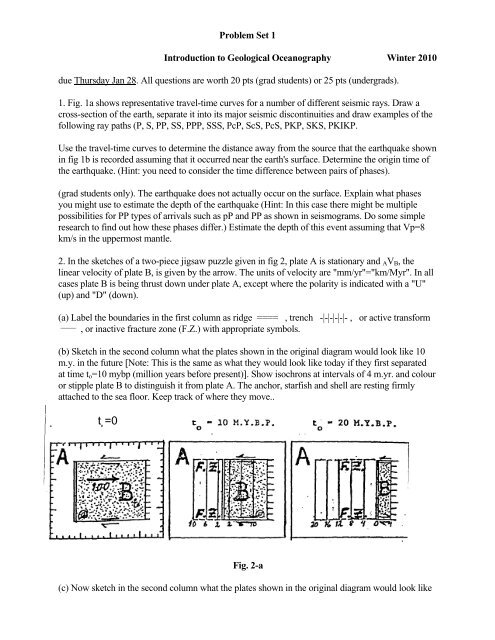
2. In the sketches of a two-piece jigsaw puzzle given in fig 2, plate A is stationary and AVB, the
linear velocity of plate B, is given by the arrow. The units of velocity are "mm/yr"="km/Myr". In all
cases plate B is being thrust down under plate A, except where the polarity is indicated with a "U"
(up) and "D" (down).
(a) Label the boundaries in the first column as ridge ==== , trench -|-|-|-|-|- , or active transform
_____ , or inactive fracture zone (F.Z.) with appropriate symbols.
(b) Sketch in the second column what the plates shown in the original diagram would look like 10
m.y. in the future [Note: This is the same as what they would look like today if they first separated
at time to=10 mybp (million years before present)]. Show isochrons at intervals of 4 m.yr. and colour
or stipple plate B to distinguish it from plate A. The anchor, starfish and shell are resting firmly
attached to the sea floor. Keep track of where they move..
t=0
0
Fig. 2-a
(c) Now sketch in the second column what the plates shown in the original diagram would look like

20 m.y. in the future. Don't be reluctant to use a pair of scissors - even the experts do!
3. Magnetic lineations in the north-eastern Pacific, which impinge upon the Aleutian trench (fig 3),
appear to form an oblique angle known as the "Great Magnetic Bight" or GMB (fig 4).
(a) Two profiles across these anomalies and on either side of the GMB are shown in fig 5, together
with models simulated from the magnetic reversal time scale. Identify these anomalies using the
magnetic reversal time scale shown in lecture 4 Figure 20 and Table 1. Use your knowledge (or the
work of others: which is to say in the readings!) to give an estimated age before attempting a detailed
identification. Remember that in trying to identify the anomalies you are looking for a particular
pattern (ie time series) of reversals to match with the model. Using the ages of these identifications,
calculate the spreading rate and spreading direction of the ridge.
(b) These calculations predict that the spreading centre that produced these anomalies subducted
beneath the Aleutian trench in the geologic past. Which sketch in Problem 2 represents a similar
situation? What do you think the geologic consequences of this might have been? Where else have
such events occurred in the geologic past? Where is a similar event occurring now?
4. An oceanographic research vessel takes a heat-flow measurement, which gives the following
results:
Depth Temperature Conductivity
m °C W/m-K
0.00 2.000 1.000
0.45 2.021 0.985
0.90 2.043 0.830
1.35 2.081 0.870
1.80 2.112 0.891
2.25 2.138 0.899
2.70 2.157 0.905
3.15 2.197 0.853
3.60 2.228 0.839
4.00 2.258 0.883
(a) What is the geothermal heat flow from these measurements, as determined by the mean
conductivity and temperature gradient over the entire depth range (0-4m)?
(b) What is the age of the ocean floor assuming that there is no error in the measurement? What
depth is expected for this age?
(c) (grad students only) The heat flow value actually has an error of +/- 5%. What error would there
be in expected age and water depth? Assuming that we can measure basement depth to an
accuracy of about +/- 50 m, what error would that produce in the estimate of age?
5. (grad students only) The mean heat loss at the earth's surface has been estimated at 3.05 x 10 13 W.
Estimate what percentage of this comes from ocean crust 0-15 Myr old. Assume that the total length
of the mid-ocean ridge system is 50,000 km and assume that it is spreading at an average total rate of
6 cm/yr (i.e. 3 cm/yr on each side).
(a) Calculate the amount of conductive heat loss from crust 0-15 Myr old that is predicted from the
theoretical model of a cooling plate. You can calculate this by integrating the equation for heatflow

as a function of time [ q = 470/sqrt(t)], where q is in mW/m 2 and t is in m.y. [If your integral calculus
is too rusty, you can proceed by discrete summation of average values for each m.y., ie 0-1, 1-2, etc.
In this case, avoid the problem of infinite heat flow at t=0 by assuming an average flow of 920
mW/m 2 for crust 0-1 Myr old, which is what more complex theories predict.]
(b) Use the data for fast spreading ridges shown in lecture 6 Figure 2a to determine the amount of
conductive heat loss from 0-15 Myr old crust that is actually observed. Why is this less than
predicted by the theoretical models?

Fig 1A
Fig 1B. Each time mark represents 1 minute. Z,N,E represent the 3 components of
the seismometers. Note that the time marks in part A are offset for the various
components. Part B represents a more detailed image of the initial arrivals.

Fig. 5
Fig. 3
Fig. 4