Operational Amplifier Stability - En-genius.net
Operational Amplifier Stability - En-genius.net
Operational Amplifier Stability - En-genius.net

You also want an ePaper? Increase the reach of your titles
YUMPU automatically turns print PDFs into web optimized ePapers that Google loves.
<strong>Operational</strong> <strong>Amplifier</strong> <strong>Stability</strong><br />
Part 1 of 15: Loop <strong>Stability</strong> Basics<br />
by Tim Green<br />
Strategic Development <strong>En</strong>gineer, Burr-Brown Products from Texas Instruments Incorporated<br />
Wherever possible the overall technique used for this series will be "definition by example" with<br />
generic formulae included for use in other applications. To make stability analysis easy we will use<br />
more than one tool from our toolbox with data sheet information, tricks, rules-of-thumb, SPICE<br />
Simulation, and real-world testing all accelerating our design of stable operational amplifier (op amp)<br />
circuits. These tools are specifically targeted at voltage feedback op amps with unity-gain bandwidths<br />
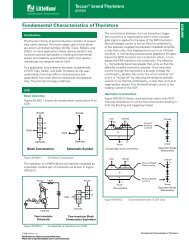
Magnitude Plot<br />
Phase Plot<br />
Fig. 1.1: Magnitude And Phase Bode Plots<br />
Magnitude Bode Plots require voltage gain to be converted to dB, defined as 20Log1010A, where A is<br />
the voltage gain in volts/volts (V/V).<br />
dB A(dB) = 20Log 10 A where A = Voltage Gain in V/V<br />
A (V/V)<br />
0.001<br />
0.01<br />
0.1<br />
1<br />
10<br />
100<br />
1,000<br />
10,000<br />
100,000<br />
1,000,000<br />
10,000,000<br />
A (dB)<br />
-60<br />
-40<br />
-20<br />
0<br />
20<br />
40<br />
60<br />
80<br />
100<br />
120<br />
140<br />
Fig. 1.2: dB Definition For Magnitude Bode Plots
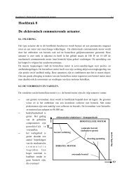
Fig. 1.3 defines some commonly-used Bode plot terms.<br />
Roll-Off Rate Decrease in gain with<br />
frequency<br />
Decade x10 increase or x1/10 decrease<br />
in frequency. From 10Hz to 100Hz is<br />
one decade.<br />
Octave X2 increase or x1/2 decrease in<br />
frequency. From 10Hz to 20Hz is one<br />
octave.<br />
Fig. 1.3: More Bode Plot Definitions<br />
The slope of voltage gain with frequency is defined in +20 dB/decade or -20 dB/decade increments on<br />
a magnitude Bode plot. They can also be described as +6 dB/octave or -6 dB/octave (see Fig. 1.4)<br />
which can be proved by:<br />
∆A (dB) = A (dB) at fb - A (dB) at fa<br />
∆A (dB) = [Aol (dB) - 20log10(fb/f1)] - [Aol (dB) - 20log10(fa/f1)]<br />
∆A (dB) = Aol (dB) - 20log10(fb/f1) - Aol (dB) + 20log10(fa/f1)<br />
∆A (dB) = 20log10(fa/f1) - 20Log10(fb/f1) = 20log10(fa/fb) = 20log10(1 k/10 k)<br />
so, ∆A (dB) = -20 dB/decade<br />
Also, ∆A (dB) = 20log10(fb/fc) = 20log10(10 k/20 k)<br />
so, ∆A (dB) = -6 dB/octave<br />
That is, -20 dB/decade = -6 dB/octave<br />
And also: +20 dB/decade = +6 dB/octave; -20dB/decade = -6dB/octave<br />
And: +40 dB/decade = +12 dB/octave; -40 dB/decade = -12 dB/octave<br />
And: +60 dB/decade = +18 dB/octave; -60 dB/decade = -18 dB/octave<br />
A (dB)<br />
Fig. 1.4: Magnitude Bode Plot: 20 dB/Decade = 6 dB/Octave
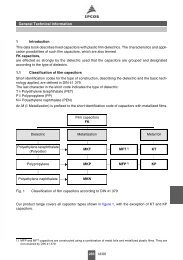
Pole<br />
A single pole response has a -20 dB/decade, -6 dB/octave rolloff in the Bode magnitude plot. At its<br />
location (fP) the gain is reduced by 3dB from the dc value. In the phase plot the pole has a -45° phase<br />
shift at fP. The phase extends on either side of fP to 0° and -90° at a -45°/decade slope. A single pole<br />
may be represented by a simple RC low pass <strong>net</strong>work as shown in Fig. 1.5. Note how the phase of a<br />
pole affects frequencies up to one decade above and one decade below the pole frequency.<br />
Zero<br />
Pole Location = f P<br />
Fig. 1.5: Poles: Bode Plot Magnitude and Phase<br />
Magnitude = -20dB/Decade Slope<br />
Slope begins at fP and continues down<br />
as frequency increases<br />
Actual Function = -3dB down @ fP Phase = -45°/Decade Slope through f P<br />
Decade Above fP Phase = -90°<br />
Decade Below fP Phase = 0°<br />
A single zero response has a +20 dB/decade, +6 dB/octave "roll-up" in the Bode magnitude plot. At<br />
the zero location (fZ) the gain is increased by 3 dB from the dc value. In the phase plot the zero has a<br />
+45° phase shift at fZ. The phase extends on either side of fZ to 0° and +90° at a +45°/decade slope. A<br />
single zero may be represented by a simple RC high pass <strong>net</strong>work (Fig. 1.6). Note how the phase of a<br />
zero affects frequencies up to one decade above and one decade below the zero frequency.
Fig. 1.6: Zeros: Bode Plot Magnitude and Phase<br />
On a Bode magnitude plot it is easy to find the frequency location of a given pole or zero. Since the xaxis<br />
is a log scale of frequency this technique allows a ratio of distances to accurately and quickly<br />
determine the frequency of the pole or zero of interest. Fig. 1.7 illustrates this "Log Scale Trick."<br />
A (dB)<br />
Fig. 1.7: Log Scale Trick<br />
Zero Location = f Z<br />
Magnitude = +20dB/Decade Slope<br />
Slope begins at fZ and continues up as<br />
frequency increases<br />
Actual Function = +3dB up @ fZ Phase = +45°/Decade Slope through f Z<br />
Decade Above fZ Phase = +90°<br />
Decade Below fZ Phase = 0°<br />
Log Scale Trick (f P = ?):<br />
1) Given: L = 1cm; D = 2cm<br />
2) L/D = Log 10 (f P )<br />
3) f P = Log 10 -1 (L/D) = 10 (L/D)<br />
f P = 10 (L/D) = 10 (1cm/2cm) = 3.16<br />
4) Adjust for the decade range<br />
working within –<br />
10Hz-100Hz decade <br />
f P = 31.6Hz<br />
5) L = Log 10 (fp’) x D<br />
L = Log 10 (3.16) x 2cm = 1cm<br />
where fp’ = fp normalized to the<br />
1-10 decade range –<br />
f P = 31.6 f P ’ = 3.16
Intuitive Component Models<br />
Most op amp applications use combinations of four key components-- op amp, resistor, capacitor, and<br />
inductor -- and to facilitate stability analysis it is convenient to have "intuitive models" for them.<br />
Our intuitive op amp model for ac stability analysis is defined in Fig. 1.8. The differential voltage<br />
between the IN+ and IN- terminals will be amplified by x1 and converted to a single-ended ac voltage<br />
source, VDIFF, which is then amplified by K(f) (representing the data sheet Aol Curve: open-loop gain<br />
vs frequency). The resultant voltage, VO, is then followed by the open-loop, ac small-signal, output<br />
resistance, RO, with the output voltage appearing as VOUT.<br />
Fig. 1.8: Intuitive Op Amp Model<br />
Our intuitive resistor model for ac stability analysis is defined in Fig. 1.9. The resistor has a constant<br />
resistance value regardless of the operating frequency.<br />
T<br />
Resistance (ohms)<br />
1.00k<br />
750.00<br />
500.00<br />
250.00<br />
R(f) Magnitude<br />
0.00<br />
1 10 100 1k 10k 100k 1M 10M 100M<br />
Frequency (Hz)<br />
Fig. 1.9: Intuitive Resistor Model<br />
+<br />
AM1<br />
+<br />
VG1<br />
A<br />
R(f) = VR / AM1<br />
VR<br />
R1 1k
Our intuitive capacitor model for ac stability analysis is defined in Fig. 1.10 and contains three distinct<br />
operating areas. At dc the capacitor is open-circuit. At "high" frequencies it is short-circuit. In between<br />
the capacitor is a frequency-controlled resistor with a 1/XC decrease in impedance as frequency<br />
increases. The SPICE simulation in Fig. 1.11 depicts our intuitive capacitor model over frequency.<br />
T<br />
XC(ohms)<br />
200.00G<br />
150.00G<br />
100.00G<br />
50.00G<br />
0.00<br />
DC X C<br />
XC(f) Magnitude<br />
DC < X C < Hi-f<br />
Fig. 1.10: Intuitive Capacitor Model<br />
Hi-f X C<br />
1 10 100 1k 10k<br />
Frequency (Hz)<br />
100k 1M 10M 100M<br />
+<br />
AM1<br />
+<br />
VG1<br />
A<br />
XC(f) = VR / AM1<br />
Fig. 1.11: Intuitive Capacitor Model SPICE Simulation<br />
VR<br />
C1 1p
Our intuitive inductor model for ac stability analysis is defined in Fig. 1.12 with three distinct<br />
operating areas. At dc the inductor is short-circuit. At "high" frequencies it is open-circuit. In between<br />
the inductor is a frequency-controlled resistor with an XL increase in impedance as frequency<br />
increases. The SPICE simulation in Fig. 1.13 depicts our intuitive inductive model over frequency.<br />
T<br />
XL(ohms)<br />
6.50M<br />
4.88M<br />
3.25M<br />
1.63M<br />
0.00<br />
+<br />
DC X L<br />
VG1<br />
AM1<br />
+<br />
A<br />
XL (f ) = VL / AM1<br />
Fig. 1.12: Intuitive Inductor Model<br />
L1 10mH<br />
VL<br />
DC < X L < Hi-f<br />
Hi-f X L<br />
1.00 10.00 100.00 1.00k 10.00k<br />
Frequency (Hz)<br />
100.00k 1.00M 10.00M 100.00M<br />
Fig. 1.13: Intuitive Inductor Model SPICE Simulation
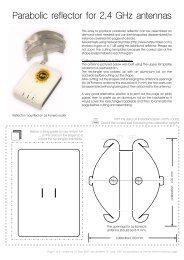
<strong>Stability</strong> Criteria<br />
The lower part of Fig. 1.14 illustrates the traditional control-loop model which represents a gain circuit<br />
with feedback. The top part of Fig. 1.14 depicts the sections of a typical op amp circuit with feedback<br />
which correspond to the control-loop model. This model can be called the op amp loop-gain model.<br />
Note that the Aol is the op amp data sheet parameter Aol, and is the open-loop gain. β is the amount of<br />
output voltage, VOUT, that gets fed back, created in this example by a resistor <strong>net</strong>work. Deriving<br />
VOUT/VIN we see that the closed-loop gain function is directly defined by Aol and β.<br />
V IN<br />
+<br />
-<br />
<strong>net</strong>work<br />
RI<br />
V FB<br />
V IN<br />
+<br />
-<br />
-<br />
+<br />
RF<br />
Aol<br />
V OUT<br />
V OUT<br />
V FB<br />
<strong>net</strong>work<br />
=V FB /V OUT<br />
V OUT<br />
RF<br />
Fig. 1.14: Op amp Loop-Gain Model<br />
From this model we can derive the criteria for stability in a closed-loop op amp circuit:<br />
V OUT /V IN = Aol / (1+ Aolβ)<br />
If: Aolβ = -1<br />
Then: V OUT/V IN = Aol / 0 ∞<br />
If VOUT/VIN = ∞ Unbounded Gain<br />
Any small changes in VIN will result in large changes in VOUT which will feed<br />
back to VIN and result in even larger changes in VOUT OSCILLATIONS <br />
INSTABILITY !!<br />
Aolβ: Loop Gain<br />
Aolβ = -1 Phase shift of +180°, Magnitude of 1 (0dB)<br />
fcl: frequency where Aolβ = 1 (0dB)<br />
<strong>Stability</strong> Criteria:<br />
At fcl, where Aolβ = 1 (0dB), Phase Shift < +180°<br />
Desired Phase Margin (distance from +180° Phase Shift) > 45°<br />
Fig. 1.15: Derivation Of <strong>Stability</strong> Criteria<br />
RI<br />
VOUT /VIN = Acl = Aol/(1+Aolβ)<br />
If Aol >> 1 then Acl ≈ 1/β<br />
Aol: Open Loop Gain<br />
β: Feedback Factor<br />
Acl: Closed Loop Gain
Loop <strong>Stability</strong> Tests<br />
Since loop stability is defined by the magnitude and phase plot of loop gain (Aolβ) we analyze its<br />
magnitude and phase by breaking into the closed-loop op amp circuit, injecting a small-signal ac<br />
source into the loop, and then measuring amplitude and phase to plot the complete loop-gain picture.<br />
Fig. 1.16 shows the equivalent control-loop block diagrams for the op amp loop-gain model and the<br />
technique we will use for the loop-gain test.<br />
Fig. 1.16: Traditional Loop Gain Test<br />
Op Amp Loop Gain Model<br />
Op Amp is “Closed Loop”<br />
Loop Gain Test:<br />
Break the Closed Loop at VOUT Ground VIN Inject AC Source, VX , into VOUT Aolβ = VY /VX When analyzing a circuit built in SPICE for simulation, the traditional loop-gain test breaks the closedloop<br />
op amp circuit using an inductor and capacitor. A very large value of inductance ensures the loop<br />
is closed at dc (a requirement for SPICE simulation is to be able to calculate a dc operating point<br />
before performing an ac Analysis) but open at the ac frequencies of interest. A very large value of<br />
capacitance ensures that our ac small signal source is not connected at dc but is directly connected at<br />
the frequencies of interest.<br />
Fig. 1.17 illustrates the SPICE setup schematic for the traditional loop-gain test.
<strong>net</strong>work<br />
RI<br />
V FB<br />
V IN<br />
+<br />
-<br />
-<br />
+<br />
RF<br />
V OUT<br />
Op Amp Loop Gain Model<br />
Op Amp is “Closed Loop”<br />
SPICE Loop Gain Test:<br />
Break the Closed Loop at VOUT Ground VIN Inject AC Source, VX , into VOUT Aolβ = VY /VX Fig. 1.17: Traditional Loop-Gain Test: SPICE Setup<br />
Before simulating a circuit in SPICE we want to know the approximate outcome. Remember GIGO<br />
(garbage-in-garbage-out)! β and 1/β, along with the data sheet Aol curve, provide a powerful method<br />
for first-order approximation of loop-gain analysis. In future sections tricks and rules-of-thumb will be<br />
presented for computing β and 1/β. Fig. 1.18 defines the β <strong>net</strong>work for op amp circuits.<br />
Fig. 1.18: Op Amp β Network
The 1/β plot imposed on the Aol curve will provide a clear picture of exactly what the loop-gain (Aolβ)<br />
plot is. From the derivation in Fig. 1.19 we clearly see that the Aolβ magnitude plot is simply the<br />
difference between Aol and 1/β when we plot 1/β in dB. Note that as frequency increases Aolβ<br />
decreases. Aolβ is the gain left to correct for errors in the VOUT/VIN or closed-loop response, so as Aolβ<br />
decreases the VOUT/VIN response will become less accurate until Aolβ goes to 0 dB when the VOUT/VIN<br />
response simply follows the Aol curve.<br />
Plot (in dB) 1/β on Op Amp Aol (in dB)<br />
Open Loop Response<br />
Aol<br />
Aolβ = Aol(dB) – 1/β(dB)<br />
100<br />
Note how Aolβ changes with frequency<br />
80<br />
60<br />
40<br />
20<br />
0<br />
1<br />
10<br />
Aol<br />
(Loop Gain)<br />
100<br />
1k<br />
10k<br />
Frequency (Hz)<br />
Proof (using log functions):<br />
20Log10 [Aolβ] = 20Log10 (Aol) - 20Log10 (1/β)<br />
= 20Log10 [Aol/(1/β)]<br />
= 20Log10[Aolβ]<br />
100k<br />
Closed Loop Response<br />
fcl Acl<br />
1M<br />
10M<br />
Fig. 1.19: Loop Gain Information From Aol Plot And 1/β Plot<br />
Plotting the 1/β on the Aol curve there is an easy first-order check for stability called rate-of-closure,<br />
defined as the "rate-of-closure" of the 1/β curve with the Aol curve at fcl, where the loop gain goes to<br />
0 dB. A 40 dB/decade rate-of-closure implies an UNSTABLE circuit, because it implies two poles in<br />
the Aolβ plot before fcl which can mean a 180° phase shift; a 20 dB/decade rate-of-closure implies a<br />
STABLE circuit. Four examples are shown in Fig. 1.20 with their respective rate-of-closure computed<br />
below.
fcl1: Aol - 1/β1 = -20 dB/decade - +20 dB/decade = -40 dB/decade rate-of-closure: Unstable<br />
fcl2: Aol - 1/β2 = -20 dB/decade - 0 dB/decade = -20 dB/decade rate-of-closure: Stable<br />
fcl3: Aol - 1/β3 = -40 dB/decade - 0 dB/decade = -40 dB/decade rate-of-closure: Unstable<br />
fcl4: Aol - 1/β4 = -40 dB/decade - -20 dB/decade = -20dB/decade rate-of-closure: Stable<br />
Loop Gain <strong>Stability</strong> Example<br />
At fcl: Loop Gain (Aolβ) = 1<br />
Rate-of-Closure @ fcl =<br />
(Aol slope – 1/β slope)<br />
*20dB/decade Rate-of-Closure @ fcl =<br />
STABLE<br />
**40dB/decade Rate-of-Closure@ fcl =<br />
UNSTABLE<br />
Fig. 1.20: Rate-Of-Closure Test for Loop Gain <strong>Stability</strong><br />
A loop gain analysis example (see Fig. 1.21) serves to relate how we can analyze the stability of an op<br />
amp circuit from the 1/β plot plotted on the Aol curve. As frequency increases the capacitor, CF, goes<br />
towards zero in impedance lowering the magnitude of the β plot with frequency (less voltage feedback)<br />
and raising the 1/β curve. From our rate-of-closure criteria we predict an Unstable circuit.<br />
Rate-of-Closure @ fcl = 40dB/decade<br />
UNSTABLE!<br />
Fig. 1.21: Loop Gain <strong>Stability</strong> Example
From our 1/β plot on the Aol curve we can plot the Aolβ (loop-gain) magnitude plot (see Fig. 1.22) and<br />
we can then plot the loop gain phase plot. The rules to create an Aolβ plot from the 1/β plot on the Aol<br />
curve are simple: Poles and zeros from the Aol curve are poles and zeros in the Aolβ plot. Poles and<br />
zeros from the 1/β plot are opposite in the Aolβ plot. One easy way to remember this is β is used in the<br />
Aolβ plot and 1/β is the reciprocal of β and so we would expect the Aolβ curve to use the reciprocal of<br />
poles and zeros from the 1/β plot. Reciprocal of a pole is a zero and reciprocal of a zero is a pole.<br />
At fcl:<br />
Phase Shift = -180<br />
Phase Margin = 0<br />
1/β and Closed-Loop Response<br />
180<br />
135<br />
90<br />
45<br />
0<br />
-45<br />
fp1<br />
10 100 1k 10k 100k 1M 10M<br />
fz1<br />
Frequency<br />
(Hz)<br />
To Plot Aolβ from Aol & 1/β Plot:<br />
Poles in Aol curve are poles in Aolβ (Loop Gain)Plot<br />
Zeros in Aol curve are zeros in Aolβ (Loop Gain) Plot<br />
Poles in 1/β curve are zeros in Aolβ (Loop Gain) Plot<br />
Zeros in 1/β curve are poles in Aolβ ( Loop Gain) Plot<br />
[Remember: β is the reciprocal of 1/β]<br />
Fig. 1.22: Loop Gain Plot From Aol Curve & 1/β Plot<br />
The VOUT/VIN closed-loop response is not always the same as 1/β. In the example in Fig. 1.23 we see<br />
that the ac small-signal feedback is modified by the Rn-Cn <strong>net</strong>work in parallel with RI.<br />
At fcl Aolβ = 1 (0dB).<br />
No Loop Gain left to correct for errors.<br />
VOUT /VIN follows the Aol curve.<br />
100<br />
80<br />
60<br />
40<br />
20<br />
0<br />
1<br />
10<br />
100<br />
Aol<br />
SSBW<br />
(Small Signal BandWidth)<br />
1k 10k<br />
Frequency (Hz)<br />
V OUT /V IN<br />
fcl<br />
100k<br />
1M<br />
10M<br />
Fig. 1.23: VOUT/VIN Vs 1/β<br />
fcl<br />
Note:<br />
fp2<br />
1/β is the AC Small Signal<br />
Closed Loop Gain for the<br />
Op Amp.<br />
V OUT /V IN is often NOT the<br />
same as 1/β.
As frequency increases we see the results of this <strong>net</strong>work reflected in the 1/β plot on the Aol curve.<br />
Think of this example as an inverting summing op amp circuit. We are summing in VIN through RI and<br />
ground through the Rn-Cn <strong>net</strong>work. VOUT/VIN will not be affected by this Rn-Cn <strong>net</strong>work at low<br />
frequencies and the desired gain is seen as 20 dB. As loop gain (Aolβ) is forced to 1 (0 dB) by the Rn-<br />
Cn <strong>net</strong>work there is no loop gain left to correct for errors and VOUT/VIN will follow the Aol curve at<br />
frequencies above fcl.<br />
References<br />
Frederiksen, Thomas M. Intuitive <strong>Operational</strong> <strong>Amplifier</strong>s, From Basics to Useful Applications,<br />
Revised Edition. McGraw-Hill Book Company. NY, NY. 1988<br />
Faulkenberry, Luces M. An Introduction to <strong>Operational</strong> <strong>Amplifier</strong>s With Linear IC Applications,<br />
Second Edition. John Wiley & Sons. NY, NY. 1982<br />
Tobey; Graeme; Huelsman -- Editors. Burr-Brown <strong>Operational</strong> <strong>Amplifier</strong>s, Design and Applications.<br />
McGraw-Hill Book Company. NY, NY. 1971<br />
About The Author<br />
After earning a BSEE from the University of Arizona, Tim Green has worked as an analog and mixedsignal<br />
board/system level design engineer for over 23 years, including brushless motor control, aircraft<br />
jet engine control, missile systems, power op amps, data acquisition systems, and CCD cameras. Tim's<br />
recent experience includes analog & mixed-signal semiconductor strategic marketing. He is currently a<br />
Strategic Development <strong>En</strong>gineer at Burr-Brown, a division of Texas Instruments, in Tucson, AZ and<br />
focuses on instrumentation amplifiers and digitally-programmable analog conditioning ICs.