An Algorithm for the Estimation of the Signal-To-Noise Ratio in ...

TBME-00560-2011 1
Author’s version. Published in: IEEE Trans Biomed Eng. 2012 Jan;59(1):219-25. DOI: 10.1109/TBME.2011.2170687
An Algorithm for the Estimation of the
Signal-To-Noise Ratio in Surface Myoelectric
Signals Generated During Cyclic Movements
Abstract—In many applications requiring the study of the
surface myoelectric signal (SMES) acquired in dynamic
conditions, it is essential to have a quantitative evaluation of the
quality of the collected signals. When the activation pattern of a
muscle has to be obtained by means of single- or double-
threshold statistical detectors, the background noise level (e
noise)
of the signal is a necessary input parameter. Moreover, the
detection strategy of double-threshold detectors may be properly
tuned when the signal-to-noise ratio (SNR) and the duty cycle
(DC) of the signal are known. The aim of this work is to present
an algorithm for the estimation of enoise, SNR and DC of a SMES
collected during cyclic movements. The algorithm is validated on
synthetic signals with statistical properties similar to those of
SMES, as well as on more than a hundred real signals.
Index Terms—Cyclic movements, signal-to-noise ratio (SNR),
surface electromyography (sEMG), surface myoelectric signal
(SMES).
I. INTRODUCTION
HE analysis of the myoelectric signal allows to determine
T if a specific muscle is active or silent [1]. Surface
myoelectric probes – applied on the skin above the muscle –
permit a non-invasive evaluation of the muscle activity.
The traditional use of surface myoelectric signal (SMES) in
physiological and biomechanical research [2] was extended to
applied research: SMES achieved a well established value as
an evaluation tool in surgery planning [3], rehabilitation [4],
biofeedback [5]–[6], sports medicine and training [7], and
ergonomics research [8].
Among other innovative applications, it is gaining interest
the development of advanced human–machine interfaces in
which SMES has a key role to play. In particular, myoelectric
control [9] is an advanced technique concerned with the
(c) 2011 IEEE. Personal use of this material is permitted. Permission from
IEEE must be obtained for all other users, including reprinting/ republishing
this material for advertising or promotional purposes, creating new collective
works for resale or redistribution to servers or lists, or reuse of any
copyrighted components of this work in other works."
*V. Agostini is with the Dipartimento di Elettronica, Politecnico di Torino,
10129 Torino, Italy, (phone: +39-011-5644136; fax: +39-011-5644217;
e-mail: valentina.agostini@polito.it).
M. Knaflitz is with the Dipartimento di Elettronica, Politecnico di Torino,
10129 Torino, Italy, (phone: +39-011-5644135; fax: +39-011-5644217;
e-mail: marco.knaflitz@polito.it).
Valentina Agostini and Marco Knaflitz, Member, IEEE
detection, processing, classification, and application of SMES
to the active control of prosthetic limbs, human-assisting
robots, or rehabilitation devices.
The vast majority of the above mentioned applications
evaluates muscle activity in dynamic conditions and, in
particular, during cyclic or repetitive motor tasks [10]–[12],
e.g. walking (gait analysis) [13]–[14] or biking [15]. The
movements of the corresponding body segments imply cyclic
contractions of muscles. As a consequence, SMES detected
from a specific muscle results in a sequence of pseudoperiodical
activation bursts [16]. In the time elapsed between
the end of a muscle burst and the beginning of the successive
one, the muscle under study is silent. However, the probe
detects a background noise that is unavoidable in any dynamic
test. This background noise is mainly due to crosstalk [2] from
neighboring muscles: it is a ‘physiological’ noise, more
relevant than that due to instrumentation.
In order to evaluate the quality of the recorded signals, the
background noise and the signal-to-noise ratio are usually
estimated by means of manual or automatic segmentation of
the signal in the time-domain. To this purpose, myoelectric
bursts are separated from muscle baseline activity and the
corresponding powers are calculated and compared.
In the analysis of dynamic SMES it is of paramount
importance to obtain the onset and offset time instants of a
muscle burst, distinguishing the muscle activity from the
background noise. The relevance of considering the muscle
activation timing is supported by several studies
demonstrating its usefulness in orthopedics, treatment of
cerebral palsy, and a number of other clinical applications
[13].
Well established techniques to determine the activation
pattern of a muscle are based on single- or double-threshold
statistical detectors [17]–[18]. These detectors require, as a
necessary input parameter to set the (first) threshold, the
background noise level. Furthermore, double-threshold
detectors require additional parameters in order to fine-tune
the second threshold. In particular, it is important to estimate
the signal-to-noise ratio (SNR) and, to a minor extent, the duty
cycle (DC) of the detected signal.
The method we present in this contribution allows to
estimate the root-mean-square value of the background noise
), the SNR and the DC of an SMES generated during
(enoise

TBME-00560-2011 2
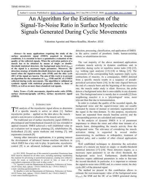
Fig. 1. Cyclo-stationary processes with enoise = 1µV and SNR = 20 dB.
Upper plots: representation of a single cycle with (a) DC = 20%, (b) DC =
50%, (c) DC = 80%. Lower plots: histograms of the amplitudes of the three
processes. The time support of the signals considered to obtain the
histograms is equal to 30 s.
cyclic movements. This is done following a statistical
approach that does not require any a priori knowledge on the
signal. In this way, we obtain the input parameters necessary
to run double-threshold algorithms without the need of preprocessing
the signal in the time domain.
II. MATERIALS AND METHODS
A. The surface myoelectric signal in cyclic movements
The SMES recorded during cyclic contractions may be
considered as the superposition of the signal generated by the
observed muscle during its contraction and the background
noise. This noise is mainly due to the activity of neighboring
muscles, collected because of the limited spatial selectivity of
the detection probe. Moreover, due to the cyclic nature of the
movement, this process may be defined as cyclostationary
[19]. Its periodicity depends on the cyclic movement under
investigation.
In its period of cyclostationarity, the signal can be modeled
as the superposition of two stationary processes: noise only,
when the muscle is not active, and a second process
corresponding to the muscle activity.
When the muscle is non-active (OFF-state) only
background noise is present. This noise can be modeled as a
Gaussian process with zero-mean and variance σ :
2
n(t) ∈ Ν(0,
σ ) . (1)
n
During muscle activity (ON-state), the SMES can be
modeled as a zero-mean Gaussian process given by the
superimposition of two Gaussian processes corresponding to
signal and background noise, respectively:
2
n
2 2
x(t) = s(t) + n(t) ∈ Ν(0,
σ + σ ) , (2)
being
2
σ s the variance of s(t).
s
The percentage of time in which the muscle is active with
respect to the total cycle duration is referred to as duty cycle.
In the following, it is assumed that the signal x(t) is sampled
with a sampling period Ts that satisfies the Nyquist criterion.
In particular, since SMES collected by means of usual surface
probes typically has more than 99% of the signal power below
500 Hz, we consider a sampling frequency fc = 2 kHz, that
results in a two-time oversampling.
B. Separating signal from noise
The probability density function of the cyclostationary
signal considered above is given by the superposition of the
probability density functions corresponding to x(t) and n(t)
and depends also on the DC. As an example, Fig. 1 reports
the histograms of three cyclostationary processes
corresponding to enoise equal to 1 µV, SNR equal to 20 dB and
DC equal to 20%, 50% and 80%, respectively.
The separation of the ON-state from the OFF-state could be
obtained by applying a proper detector, but such detectors
would require, as an input parameter, the root-mean-square
value of the background noise enoise
[18], that is unknown. A
possible solution for estimating enoise, without actually
separating the ON and OFF states in the time domain, consists
of considering an auxiliary time series with a χ 2
distribution.
The amplitude histogram of the auxiliary time series has two
separated modes, one corresponding to the noise variance and
the other to the signal variance.
The auxiliary time series Cr(k)
is obtained subdividing the
time series x(t) in M epochs constituted by r consecutive
samples and then considering the normalized sum of squares
of each epoch:
X kj
Cr
(k) = , k = 1,…,M . (3)
r
r
∑
j=
1
2
Fig. 2. Histograms of the series of the normalized sum of squares Cr (in
logarithmic scale) of a 30s-cyclostationary process with SNR = 20 dB and
DC = 50% for (a) r = 2, (b) r = 10, (c) r = 50.
n

TBME-00560-2011 3
Fig. 3. Histogram of Log10C relative to a cyclic signal with enoise = 1µV,
SNR = 20 dB and DC = 50% (time support of the signal = 30 s). The darkcolored
bars indicate the bins used by the algorithm to estimate the
parameters.
If the signal follows the hypothesized model, the time series
has a bimodal distribution with two separated modes. The
2 2
larger is the difference among σ n and σ s , the greater is the
distance between the modes.
As an example, Fig. 2 reports the bimodal distributions
obtained for r = 2, r = 10 and r = 50, respectively. It is evident
that increasing r allows for a better separation of the two
modes, but contemporarily, due to the reduced size of the
series Cr(k),
we have a reduced number of samples. Moreover,
increasing the r value causes a loss of time resolution from 1
ms (r = 2) up to 25 ms (r = 50). A satisfactory tradeoff may be
obtained by choosing r = 10 (time resolution equal to 5 ms).
This guarantees an acceptable time resolution, a good
separation between the noise and the signal modes, and a
sufficient number of samples to build the histogram.
The assumption of gaussianity of the SMES allows to treat
the auxiliary time series Cr(k)
as χ 2 -distributed. This is useful
to determine the number of consecutive samples (r) that
constitute Cr(k)
in an optimal way. However, even if the
SMES is not exactly Gaussian, the auxiliary time series will
still be two-bell shaped and the algorithm described below will
give reliable results.
C. Description of the algorithm
In order to estimate enoise,
SNR and DC of an SMES
generated during cyclic movements we use the following
algorithm:
1) Consider the time series {xi},
i = 1,…, N, being N the
number of samples. In the following, we refer to a time series
with a duration equal to 30 s sampled at sampling frequency
equal to 2 kHz. It follows that the number of samples N is
equal to 60000.
2) Divide {xi}
into M = N/r epochs. Considering r = 10 we
have:
Fig. 4. Histogram of Log10C relative to a cyclic signal with enoise = 1µV,
SNR = 6 dB and DC = 50% (time support of the signal = 30 s). The darkcolored
bars indicate the bins used by the algorithm to estimate the
parameters.
{X kj}
= {X1j,
X 2j,
…,
X Mj},
j = 1, …,10
3) Obtain the auxiliary time series of the normalized sum of
squares:
10 2
X kj
C (k) = ∑ , k = 1, …,
M .
(4)
j=
1 10
4) Obtain the histogram of the series Log10 C. The bins of
the histogram are defined as:
max( Log10C)
− min( Log10C)
bins(m) ≡ m ⋅
2 ⋅ Nbins
(5)
+ min( Log C),
m = 1,
3,...,
2 ⋅ Nbins −1.
10
where Nbins is the number of bins. Since in our case M =
6000, to have a sufficient sample numerosity for each bin we
choose Nbins = 60. In general, a number of bins in the range
50-100 is an acceptable choice.
5) Search for local maxima of the curve that interpolates the
frequencies of the histogram. Locate the absolute maximum
and the highest relative maximum. The leftmost point of
maximum is associated to noise (Inoise), the rightmost is
associated to signal (Isignal).
6) Estimate the mean power of the noise, averaging five
bins around I :
I
+ 2
noise
∑
noise
i = Inoise
−2
noise = Inoise
+ 2
P
bins(i) ⋅ Freq(i)
. (6)
∑
i = Inoise
−2
Freq(i)
7) Estimate the mean power of the signal, averaging five
bins around Isignal:

TBME-00560-2011 4
Fig. 5. Representation of 1 cycle of the synthetic SMES obtained with (a) a
rectangular window, (b) a Gaussian window with σ=1 and (c) a Gaussian
window with σ=2. In this example SNR = 20 dB and DC = 50%.
Isignal+
2
∑
i = Isignal−2
signal = Isignal+
2
P
bins(i) ⋅ Freq(i)
. (7)
∑
i = Isignal−2
Freq(i)
8) Estimate the root-mean-square value of the background
noise enoise:
e = P . (8)
noise
noise
TABLE I
RECTANGULAR WINDOW
enoise (µV)
20% 40% 60% 80%
6 dB 1.00 ± 0.01 1.00 ± 0.04 1.02 ± 0.03 1.52 ± 0.63
12 dB 1.00 ± 0.01 1.01 ± 0.03 1.00 ± 0.02 1.01 ± 0.04
18 dB 1.00 ± 0.02 1.00 ± 0.02 1.00 ± 0.02 1.00 ± 0.02
24 dB 1.01 ± 0.02 1.00 ± 0.02 1.00 ± 0.02 0.99 ± 0.01
30 dB 0.99 ± 0.02 1.00 ± 0.02 1.00 ± 0.02 1.00 ± 0.03
SNR (dB)
20% 40% 60% 80%
6 dB 5.9 ± 0.3 5.9 ± 0.5 5.7 ± 0.4 3.4 ± 3.0
12 dB 12.0 ± 0.4 11.9 ± 0.4 11.9 ± 0.2 11.9 ± 0.3
18 dB 17.9 ± 0.3 18.1 ± 0.2 17.8 ± 0.2 18.0 ± 0.3
24 dB 23.9 ± 0.2 24.0 ± 0.2 23.9 ± 0.2 24.2 ± 0.2
30 dB 30.0 ± 0.2 30.0 ± 0.2 30.0 ± 0.2 30.0 ± 0.2
DC (%)
20% 40% 60% 80%
6 dB 20.1 ± 0.7 39.6 ± 0.6 59.1 ± 0.6 80.5 ± 6.9
12 dB 19.8 ± 1.0 39.9 ± 0.7 60.2 ± 0.6 80.4 ± 0.6
18 dB 20.2 ± 0.5 40.1 ± 0.6 60.3 ± 0.6 80.3 ± 0.5
24 dB 20.2 ± 0.6 40.4 ± 0.6 60.1 ± 0.7 80.6 ± 0.6
30 dB 20.1 ± 0.4 40.2 ± 0.5 60.4 ± 0.6 80.4 ± 0.3
Estimation of background noise (enoise), signal-to-noise ratio (SNR) and
duty cycle (DC) for synthetic signals obtained with a rectangular window.
It is reported the mean value estimated over ten realizations ± its standard
deviation.
9) Estimate the SNR (in dB):
SNR
DC
P
− P
signal noise
= 10 ⋅ Log
. (9)
10
Pnoise
10) Estimate the duty cycle (%):
100
= ⋅ Isignal+
2
∑
noise
∑ Freq(i) + ∑
i = Isignal−2
Isignal+
2
i = Isignal−2
Freq(i)
TABLE II
GAUSSIAN WINDOW WITH σ = 1
enoise (µV)
20% 40% 60% 80%
6 dB 0.99 ± 0.03 1.01 ± 0.02 1.17 ± 0.31 1.60 ± 0.47
12 dB 1.00 ± 0.02 1.00 ± 0.02 0.99 ± 0.03 1.00 ± 0.04
18 dB 1.00 ± 0.02 1.00 ± 0.02 1.00 ± 0.02 1.00 ± 0.03
24 dB 1.00 ± 0.02 1.00 ± 0.02 1.00 ± 0.02 1.00 ± 0.03
30 dB 1.00 ± 0.02 0.99 ± 0.02 0.99 ± 0.03 1.00 ± 0.02
SNR (dB)
20% 40% 60% 80%
6 dB 4.5 ± 0.5 4.3 ± 0.6 3.8 ± 1.5 4.1 ± 2.2
12 dB 10.6 ± 0.4 10.6 ± 0.3 10.5 ± 0.5 10.5 ± 0.5
18 dB 16.6 ± 0.4 16.6 ± 0.4 16.5 ± 0.2 16.6 ± 0.5
24 dB 22.5 ± 0.3 22.6 ± 0.3 22.6 ± 0.2 22.6 ± 0.4
30 dB 28.5 ± 0.3 28.6 ± 0.4 28.7 ± 0.2 28.7 ± 0.2
DC (%)
20% 40% 60% 80%
6 dB 18.7 ± 0.7 37.8 ± 5.0 55.1 ± 0.8 71.8 ± 1.5
12 dB 17.7 ± 0.8 36.5 ± 0.5 56.4 ± 0.3 77.7 ± 0.7
18 dB 17.7 ± 0.5 36.1 ± 1.0 56.0 ± 0.7 77.8 ± 0.5
24 dB 17.6 ± 0.3 36.2 ± 0.5 56.1 ± 0.4 77.7 ± 0.4
30 dB 17.8 ± 0.4 36.6 ± 0.6 56.8 ± 0.6 77.7 ± 0.6
I
Estimation of background noise (enoise), signal-to-noise ratio (SNR) and
duty cycle (DC) for synthetic signals obtained with a Gaussian window
with σ=1. It is reported the mean value estimated over ten realizations ±
its standard deviation.
+ 2
i = Inoise
−2
Freq(i)
. (10)
In order to clarify how the algorithm works, Fig. 3
represents a 30s-cyclostationary signal with DC = 50% and
SNR = 20 dB. Fig. 4 reports a similar example with SNR = 6
dB. As one could have expected, in the 6dB-case there is a
partial superposition between the bell-shaped curve relative to
the noise and that relative to the signal. However, their modes
are still clearly distinguishable.
III. RESULTS AND DISCUSSION
A. Validation of the algorithm
Synthetic signals are generated with a time duration of 30 s.
They are cyclic with a cycle duration of 1 s. They are obtained
adding a random process simulating the background noise to a
process simulating the SMES generated during a muscle

TBME-00560-2011 5
contraction. Background noise is simulated as a Gaussian
process with zero mean and standard deviation equal to 1µV.
The SMES burst is generated as a Gaussian process with zero
mean and standard deviation equal to 10 (SNR/20)
∙1µV,
windowed on a time support defined by DC. In order to
simulate different muscle activation modalities we consider
three different types of windows: a) a rectangular window,
b) a Gaussian window with σ=1, c) a Gaussian window with
σ=2 (see Fig. 5).
The performances of the algorithm were verified for five
different values of the SNR (6, 12, 18, 24, 30 dB) and for four
different values of DC (20, 40, 60, 80 %).
TABLE III
GAUSSIAN WINDOW WITH σ = 2
enoise (µV)
20% 40% 60% 80%
6 dB 1.02 ± 0.03 1.05 ± 0.03 1.08 ± 0.04 1.14 ± 0.12
12 dB 1.01 ± 0.02 1.02 ± 0.01 1.05 ± 0.03 1.20 ± 0.33
18 dB 0.99 ± 0.02 1.00 ± 0.02 1.02 ± 0.02 1.49 ± 1.04
24 dB 1.00 ± 0.02 1.00 ± 0.02 1.00 ± 0.03 1.36 ± 1.36
30 dB 1.00 ± 0.02 0.99 ± 0.02 0.99 ± 0.03 1.44 ± 2.19
SNR (dB)
20% 40% 60% 80%
6 dB 4.5 ± 2.5 3.9 ± 2.0 1.2 ± 2.1 0.3 ± 2.1
12 dB 9.2 ± 1.0 9.6 ± 0.6 9.6 ± 0.8 8.2 ± 2.5
18 dB 16.6 ± 0.5 16.3 ± 0.9 16.2 ± 0.5 13.7 ± 4.9
24 dB 21.7 ± 1.0 22.1 ± 0.3 22.4 ± 0.4 21.1 ± 4.5
30 dB 28.2 ± 0.5 28.3 ± 0.5 28.4 ± 0.3 27.4 ± 4.5
DC (%)
20% 40% 60% 80%
6 dB 10.5 ± 1.6 20.9 ± 1.3 36.4 ± 8.1 46.7 ± 9.7
12 dB 10.0 ± 0.4 22.0 ± 0.8 35.6 ± 0.9 50.6 ± 1.2
18 dB 10.0 ± 0.4 22.2 ± 0.8 39.2 ± 0.8 61.3 ± 2.0
24 dB 10.1 ± 0.8 22.9 ± 0.6 39.9 ± 0.9 64.1 ± 1.1
30 dB 10.4 ± 0.4 23.3 ± 0.5 40.8 ± 0.7 64.8 ± 0.8
Estimation of background noise (enoise), signal-to-noise ratio (SNR) and
duty cycle (DC) for synthetic signals obtained with a Gaussian window
with σ=2. It is reported the mean value estimated over ten realizations ±
its standard deviation.
We considered 10 realizations of the described synthetic
signals and estimated enoise,
SNR and DC for each of them.
Then, we calculated the mean value and standard deviation of
these parameters over the 10 realizations. Table 1 reports the
results relative to the rectangular window, Table 2 those
obtained using the Gaussian window with σ = 1, and Table 3
those relative to the Gaussian window with σ = 2.
The estimated background noise (enoise)
shows values that
are almost always very close to the expected value of 1µV. In
the large majority of cases, the corresponding error is lower
than 1%. In the rectangular window case (Table 1) the
estimated SNR and DC show values that are very close to their
expected values. Again, in the large majority of simulation
conditions, the error is lower than 1%. In the case of the
Gaussian window with σ=1, there is a slight underestimation
of SNR and DC (see Table 2). This behavior is reinforced in
the case of the Gaussian window with σ=2. In fact, the
estimated values are systematically and appreciably lower than
the expected ones. This is not surprising and it is due to the
shape of the applied window. When dealing with real signals
similar to this typology, the estimated values of SNR and DC
are always underestimated.
On the contrary, when the Gaussian windows are
considered and DC is equal to 80% , the estimated value of the
background noise is overestimated up to 60% relative to its
true value. The effect of this overestimation is a slight
reduction of the sensitivity of the single- or double-threshold
detectors, that generally does not compromise their
performances.
Although the method herein presented was developed to
allow the tuning of statistical detectors, other applications are
possible. As an example, the availability of the estimates of
enoise
and SNR makes it possible to evaluate the quality of the
acquired signal in a user independent way. This is of
paramount importance to allow for a prompt detection of
signals whose quality is not high enough to guarantee reliable
results of the processing techniques applied to them.
B. Test of the algorithm on real SMES
Although the validation of the proposed algorithm was
carried out working with synthetic SMES, we tested the
algorithm also on real signals.
In order to test the applicability of the algorithm to real
SMES, recorded during cyclic human movements, we
consider - as an example - signals acquired during gait. Our
database consists of a total of 142 SMES collected from:
Fig. 6. Examples of application of the algorithm to real signals. (a) SMES
from tibialis anterior: enoise1 = 3.2 µV, SNR1 = 28.0 dB, DC1 = 37.8%. (b)
SMES from gastrocnemius lateralis: enoise1 = 1.5 µV, SNR1 = 11.3 dB,
DC1 = 44.6%.

TBME-00560-2011 6
Fig. 7. SMES segmentation in the time domain. The segments labeled as A1,
A2, … correspond to muscle activations (= ON states), while B1, B2,…
indicate background noise (= OFF states).
tibialis anterior (48), gastrocnemius lateralis (32), lateral
hamstrings (24), vastus lateralis (24), rectus femoris (14), The
SMES acquisitions were carried out positioning surface
myoelectric probes (STEP32, DemItalia, Italy) over the
muscle’s belly [1]. As for the synthetic signals, we considered
a time support of 30 s. The real signals are “pseudo-cyclic”
with a cycle duration equal to the subject gait cycle.
Fig. 6 shows an example of SMES collected from (a)
tibialis anterior and (b) gastrocnemius lateralis. The
corresponding two-bell shaped histograms are shown aside.
We estimated the parameters both with the algorithm
described above and by means of an alternative method. The
parameters estimated through the proposed algorithm will be
indicated as enoise1, SNR1, DC1, while those estimated with
the alternative procedure will be indicated as enoise2, SNR2,
DC2. The alternative procedure consists of segmenting the
30-s signals in the time domain, obtaining the ON and OFF
states by means of the double-threshold detector [18]. An
example of signal segmentation is shown in Fig. 7.
Indicating with N the number of segmented gait cycles we
define:
N
1
e noise2 ≡ ∑ σ Bi ,
(11)
N i = 1
where σ Bi is the standard deviation of the i-th background
noise segment (see Fig. 7).
Furthermore, we define:
2
A
NR2 10 log 10 1 ,
2 ⎟
B
⎟
⎛ σ ⎞
S ≡ ⋅ ⎜
−
(12)
⎝ σ ⎠
2
A
2
σ B are the mean variances of the ON and OFF
where σ and
states, respectively.
Finally, we define:
N
1 Ai
D C2 ≡ ∑ ⋅ 100.
(13)
N i = 1 Ai
+ Bi
Fig. 8 shows the comparison of the two methods on the set
of 142 real signals. This figure displays, for each parameter,
the scatter plot of the values obtained with the proposed
algorithm (x-axis) and with the alternative method (y-axis). To
determine how well the proposed algorithm retrieves the
values obtained with the “direct” time-domain method we
calculated the regression line among the points. The line
among enoise1-enoise2 points has a slope close to 1 (0.97)
and a very small y-intercept (0.41 µV rms), demonstrating the
accuracy of the proposed algorithm in the estimation of
background noise. Results are still acceptable when
considering the SNR1-SNR2 scatter plot, also if it can be
noticed a slight underestimation of SNR1 with respect to
SNR2. For what concerns the duty cycle the values obtained
with the algorithm are systematically lower than those
obtained with the alternative method of about 20% of the gait
cycle. These findings are similar to those already commented
for the synthetic signals with Gaussian window with σ=1 and,
more markedly, in the case σ=2.
IV. CONCLUSION
This work presents an algorithm for the estimation of
background noise, signal-to-noise ratio and duty cycle of
SMES generated during cyclic movements. The algorithm was
tested on synthetic and real SMES and the obtained results
show that, in most practical situations, it provides accurate and
stable measures of the aforementioned parameters.
We adopted this method to choose the parameters of a
double-threshold statistical detector we previously developed
[18] and that we have been using in the past years to carry-out
a user independent analysis of the SMES detected during
walk. Results we obtained in that field are fully satisfactory
and we believe that the approach herein presented could be
beneficial also in other applications, when dealing with
operator independent processing of SMES or other biomedical
Fig. 8. Scatter plots illustrating the comparison between the two methods. Each point in the plots represents the values of the parameters estimated with: (1) the
proposed algorithm (x-axis) and (2) the time-domain method (y-axis), respectively. In each plot the regression line is shown superimposed as well as its
corresponding equation.

TBME-00560-2011 7
signals with similar characteristics.
REFERENCES
[1] J. V. Basmajian and C. J. De Luca, Muscles Alive: Their Functions
Revealed by Electromyography, 5th ed., Williams & Wilkins, Baltimore
MD, 1985.
[2] C. J. De Luca, “The Use of Surface Electromyography in
Biomechanics”, Journal of Applied Biomechanics, vol. 13, no. 2, pp.
135–163, 1997.
[3] D. Patikas, S. I. Wolf, W. Schuster, P. Armbrust, T. Dreher, L.
Döderlein L. “Electromyographic patterns in children with cerebral
palsy: do they change after surgery?”, Gait Posture, vol. 26, no. 3, pp.
362–71, 2007.
[4] M. G. Benedetti, F. Catani, T. W. Bilotta, M. Marcacci, E. Mariani, S.
Giannini, “Muscle activation pattern and gait biomechanics after total
knee replacement”, Clin. Biomech., vol. 18, pp. 871–876, 2002.
[5] M. A. Crary, M. E. Groher, “Basic Concepts of Surface
Electromyographic Biofeedback in the Treatment of Dysphagia”, Am. J.
Speech Lang. Pathol., vol. 9, pp. 116–125, May 2000.
[6] R. Neblett, Y. Perez, “Surface Electromyography Biofeedback Training
to Address Muscle Inhibition as an Adjunct to Postoperative Knee
Rehabilitation”, Biofeedback, vol. 38, no. 2, pp. 56–63, Special Issue,
Summer 2010.
[7] R. Zory, F. Molinari, M. Knaflitz, F. Schena, A. Rouard, “Muscle
fatigue during cross country sprint assessed by activation patterns and
electromyographic signals time–frequency analysis”, Scand. J. Med. Sci.
Sports, doi: 10.1111/j.1600-0838.2010.01124.x, in press, 2010.
[8] G. M. Hägg, A. Luttmann, M. Jäger, “Methodologies for evaluating
electromyographic field data in ergonomics, J. Electromyogr. Kinesiol.,
vol. 10, pp. 301–312, 2000.
[9] M. A. Oskoei, H. Hu, “Myoelectric control systems—A survey”,
Biomedical Signal Processing and Control, vol. 2, pp. 275–294, 2007.
[10] P. Bonato, S. H. Roy, M. Knaflitz, C. J. De Luca, “Time-Frequency
Parameters of the Surface Myoelectric Signal for Assessing Muscle
Fatigue during Cyclic Dynamic Contractions”, IEEE Trans. Biomed.
Eng., vol. 48, no. 7, pp. 745–753, 2001.
[11] S. H. Roy, P. Bonato, M. Knaflitz, “EMG assessment of back muscle
function during cyclical lifting”, Journal of Electromyography and
Kinesiology, vol. 8, no. 4, pp. 233–245, 1998.
[12] P. Bonato, P. Boissy, U. Della Croce, S. H. Roy, “Changes in the surface
EMG signal and the biomechanics of motion during a repetitive lifting
task”, IEEE Trans. Neural Syst. Rehabil. Eng., vol. 10, pp. 38–47, 2002.
[13] Perry J. Gait analysis. Normal and pathological function. Slack
Incorporated, Thorofare NJ, 1992.
[14] C. Frigo, P. Crenna, “Multichannel SEMG in clinical gait analysis: a
review and state-of-the-art”, Clin. Biomech., vol. 24, pp. 236-245, 2009.
[15] M. Knaflitz, F. Molinari, “Assessment of Muscle Fatigue During
Biking”, IEEE Trans. Neural Syst. Rehabil. Eng., vol. 11, no. 1, pp. 17–
23, Mar. 2003.
[16] J.-N. Helal, J. Duchene, “A Pseudoperiodic Model for Myoelectric
Signal During Dynamic Exercise”, IEEE Trans. Biomed. Eng., vol. 36,
no. 11, pp. 1092–1097, 1989.
[17] G. Staude, C. Flachenecker, M. Daumer, W. Wolf, “Onset detection in
surface electromyographic signals: a systematic comparison of
methods”, EURASIP J. Appl. Signal Process., vol. 2, pp. 67–81, 2001.
[18] P. Bonato, T. D’Alessio, M. Knaflitz, “A statistical method for the
measurement of muscle activation intervals from surface myoelectric
signal during gait”, IEEE Trans. Biomed. Eng., vol. 45, pp. 287–299,
1998.
[19] W. A. Gardner, A. Napolitano, L. Paura, “Cyclostationarity: Half a
century of research”, Signal Processing, vol. 86, pp. 639–697, 2006.
Valentina Agostini was born in Rome, Italy, on
November 2, 1970. She received the Italian Laurea
in physics summa cum laude from the University of
Torino, Torino, Italy, in 1995 and the Ph.D. degree
in physics from Politecnico di Torino, Torino, Italy,
in 2002.
Since 2004 she is with the Dipartimento di
Elettronica of Politecnico di Torino, Torino, Italy, as
Research Assistant. She focused her research
interests in medical imaging and biomedical signal
processing since 2004. She worked at the evaluation of the signal-to-noise
ratio of infrared image sequences and at the motion artifact reduction in breast
dynamic infrared imaging. Her current research interests are in statistical gait
analysis and static posturography.
Marco Knaflitz (M’92) was born in Turin, Italy, on
January 20, 1955. He received the Italian Laurea in
electrical engineering and the Ph.D. in electrical
engineering from Politecnico di Torino, Torino,
Italy. From 1986 to 1990 he was with the
Neuromuscular Research Center of Boston
University, Boston, MA, as Research Assistant
Professor. From 1995 to 2000 he was appointed
Adjunct Professor at the Union Institute of
Cincinnati (OH). Since 1990 he has been with the
Dipartimento di Elettronica of Politecnico di Torino, Torino, Italy, where he is
presently Full Professor of Biomedical Engineering and he teaches
Biomedical Instrumentation and Implantable Active Devices.
He has been active since 1985 in the fields of design of biomedical
instrumentation and biomedical signal analysis. Specifically, his research
interests are mainly focused on the detection and analysis of the myoelectric
signal for research and clinical applications.
Prof. Knaflitz is a member of GNB, the Italian national group of
bioengineering.