“Are We There Yet?” Visual Tracking of Visitors ... - Ken Goldberg

“Are We There Yet?” 

Visual Tracking of Visitors Under 

Variable-Lighting Conditions for a Responsive 

Audio Art Installation 

Andrew B. Godbehere and Ken Goldberg 

University of California at Berkeley 

Abstract. For a responsive audio art installation in a skylit atrium, 

we developed a single-camera statistical segmentation and tracking algorithm. 

The algorithm combines statistical background image estimation, 

per-pixel Bayesian segmentation, and an approximate solution to the 

multi-target tracking problem using a bank of Kalman filters and Gale- 

Shapley matching. A heuristic confidence model enables selective filtering 

of tracks based on dynamic data. Experiments suggest that our algorithm 

improves recall and F2-score over existing methods in OpenCV 2.1. We 

also find that feedback between the tracking and the segmentation systems 

improves recall and F2-score. The system operated effectively for 

5-8 hours per day for 4 months. Source code and sample data is open 

source and available in OpenCV. 

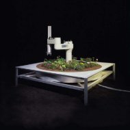
Fig. 1. The skylit atrium that was the site for this installation at the Contemporary 

Jewish museum in San Francisco, CA from April - July 2011.

2 Are We There Yet? 

1 Introduction 

1.1 Artistic Overview 

The responsive audio art installation “Are We There Yet? : 5,000 Years of Answering 

Questions with Questions” was on exhibit at the Yud gallery of the 

Contemporary Jewish Museum in San Francisco, CA from March 31 – July 31, 

2011. 

As conceived by Ken Goldberg & Gil Gershoni, “Questioning is at the core 

of Jewish cultural and spiritual identity. Jews instinctively question assumptions 

and authorities. Jewish mothers teach that ‘it never hurts to ask,’ and a Yiddish 

proverb states ‘One who doesn’t ask, doesn’t know.’ Supported by a major 

competitive grant from the Creative Work Fund, ’Are We There Yet?’ was a 

reactive sound environment where each visit was a unique mix of play, poetry, 

and contemplation.” 

The installation evoked an early stage in Jewish history when the open desert 

created opportunity for revelation; it presented new perspectives on the fundamental 

search and questioning that lies at the heart of Jewish identity. The Yud 

Gallery, designed by Daniel Libeskind and depicted in Figures 1 and 2, acknowledges 

the 2nd Commandment, emphasizing the auditory over the visual. For the 

installation, speakers were strategically positioned to preserve the open gallery 

space. Visitors experienced the work as a responsive sequence of questions that 

encouraged movement throughout the space to explore, discover, and consider. 

The project was also inspired by the Talmudic representation of multi-layered 

Jewish intellectual discourse. The Talmud is a surprisingly contemporary model 

for communal conversation in the digital age. Rather than resolving each issue 

with an authoritative unified “answer,” each page of the Talmud reflects the spiraling 

layers of debate and celebrates the dissent at the heart of Jewish thought 

and tradition. Open inquiry is fundamental to electronic connectivity and social 

networking: the culture of new media encourages participation and a natural 

skepticism about the authenticity and authority of information. 

The image in Figure 1 depicts a view of the Yud Gallery from its entrance. 

Of both artistic and technical interest are the myriad skylights, yielding very 

dynamic and atmospheric natural lighting. The illustration in Figure 2 depicts a 

schematic of the installation design and its spatial configuration, which accompanied 

the press release. 

Launched in advance of the exhibition, the “Are We There Yet?” companion 

website (http://www.are-we-there-yet.org) gave viewers the chance to learn 

more about the show, suggest their own questions for inclusion in the exhibition, 

and visually explore the suggestions of others. In the gallery space, a kiosk with 

a custom iPad interface and live, streaming interactive projection system gave 

visitors an opportunity to submit their own questions. 

We developed a state-of-the-art computer vision system and a coupled interactive 

sound system for the installation. The computer vision system detected 

and monitored the position of visitors in the space and used that information 

to trigger hundreds of pre-recorded audio files containing questions spoken by

“Are We There Yet?” 3 

people of all ages. A single fixed camera mounted on the ceiling of the gallery provided 

visual coverage. To address the challenges of constantly changing lighting 

conditions and the slight background noise produced by the camera, we developed 

an adaptive statistical background subtraction algorithm. Outliers (foreground 

pixels) in each frame are defined statistically, and grouped together into 

connected components (blobs). Our system rejected small blobs while considering 

larger blobs candidates for visitors. Dynamic information, based on interframe 

consistency (and the notion that visitors don’t move very rapidly) helped 

to further reject noise. 

1.2 Reviews 

A 2-minute video describing the installation is available at 

http://j.mp/awty-video-hd, and project reviews and documentation are available 

at http://are-we-there-yet.org. Below is a sample of press reviews. 

– Jonathan Curiel, SF Weekly Art Review [43]: “The contemplative 

walk is rightfully celebrated as a ritual of high importance, and here, at last, 

is the perfect museum hybrid: an audio-visual exhibition that asks visitors 

thought-provoking questions...getting the words out in midstroll – in a skylit 

room designed by Daniel Libeskind, no less – is an exceptional blessing.” 

– David Pescovitz, BoingBoing [44]: “The project pulls a thread dating 

back thousands of years through Jewish culture and weaves it with innovative 

digital technology to create a unique, playful, poetic, and perhaps even 

spiritual experience as you wander the room.” 

– Emily Savage, J-Weekly Review [48]: “...The walls are white and bare, 

and the only sensation is crisp, clear sound... the sensation isn’t like one 

you’ve felt before.” 

– Glenn Rosenkrantz, Covenant Foundation [53]: “Take the ages-old 

Jewish impulse to question and challenge. Add 21st century technology. And 

mix it up a bit with educators emerging embrace of new media. The result 

is potent.” 

– Molly Samuel, CNN [42]: “A new exhibit at the Contemporary Jewish 

Museum in San Francisco doesn’t just challenge visitors. It questions them... 

Cameras track each visitor, then a computer uses statistical models to understand 

who is where, where they’ve been, and where they’re heading.” 

– Huffington Post [52]: “...Gershoni and Goldberg have ingeniously made 

the scope as open as possible, anyone with internet access can paticipate, 

question, challenge, and create.” 

– Sarah Adler, SF Chronicle [45]: “...Everyone who attends is encouraged 

to submit questions to be added to the ever-evolving exhibit. The project is 

not about finding answers, but rather about learning how many questions 

remain undiscovered.” 

– Stephanie Orma, SF Weekly [46]: “Bay Area artists Ken Goldberg and 

Gil Gershoni challenge us to slow down, ask questions, and embrace contemplation. 

For they believe that it’s questions – not answers – that help us 

understand the past and propel us forward in society and in our lives.”


– Nirmala Nataraj, SF Chronicle Interview [47]: “...The questions in the 

new show range from innocuous to involved, tangential to urgent...” 

– Molly and Seth Samuel, KALW NPR [49] : “...The exhibit is designed 

so every visitor hears a different combination of questions. the room seems 

to know exactly where I am. It feels like the questions are following me as I 

walk around.” 

– Carmen Winant, KQED Arts Review [50]: “...it taps into an element 

of Judaism and Jewishness not often considered in the public sphere....the 

best exhibitions are always the ones that provoke the most questions.” 

– DesignBoom Magazine Review [54]: “The worlds of cultural tradition 

and technology mediation are brought together in Are We There Yet...” 

– Ryan White, Mill Valley Herald [51]: “...the spirit of inquisitiveness 

endures longer than the individual questions. Hasn’t compelling art always 

been more preoccupied with the asking of questions than the disclosure of 

answers?” 

1.3 Technical Overview 

In the remainder of this chapter, we present the design of a computer vision 

system that separates video into “foreground” and “background”, and subsequently 

segments and tracks people in the foreground while being robust to 

variable lighting conditions. Using video collected during the operation of the 

installation, under variable illumination created by myriad skylights, we demonstrate 

a marked performance improvement over existing methods in OpenCV 

2.1. The system runs in real-time (15 frames per second), requires no training 

datasets or calibration (unlike feature-based machine learning approaches [38]), 

and uses only 2–5 seconds of video to initialize. 

Our system consists of two stages: first is a probabilistic foreground segmentation 

algorithm that identifies possible foreground objects using Bayesian 

inference with an estimated time-varying background model and an inferred 

foreground model, described in Section 2. The background model consists of 

nonparametric distributions on RGB color-space for every pixel in the image. 

The estimates are adaptive; newer observations are more heavily weighted than 

old observations to accommodate variable illumination. The second portion is 

a multi-visitor tracking system, described in Section 3, which refines and selectively 

filters the proposed foreground objects. Selective filtering is achieved with 

a heuristic confidence model, which incorporates error covariances calculated by 

the multi-visitor tracking algorithm. For the tracking subsystem, in Section 3, we 

apply a bank of Kalman filters [18] and match tracks and observations with the 

Gale-Shapley algorithm [13], with preferences related to the Mahalanobis distance 

weighted by the estimated error covariance. Finally, a feedback loop from 

the tracking subsystem to the segmentation subsystem is introduced: the results 

of the tracking system selectively update the background image model, avoiding 

regions identified as foreground. Figure 3 illustrates a system-level block diagram. 

Figure 2 offers an example view from our camera and some visual results 

of our algorithm.


The operating features of our system are derived from the unique requirements 

of an interactive audio installation. False negatives, i.e. people the system 

has not detected, are particularly problematic because the visitors expect 

a response from the system and become frustrated or disillusioned when the 

response doesn’t come. Some tolerance is allowed for false positives, which add 

audio tracks to the installation; a few add texture and atmosphere. However, 

too many false positives creates cacophony. Performance of vision segmentation 

algorithms is often presented in terms of precision and recall [30]; many false 

negatives corresponds to a system with low recall. Many false positives lowers 

precision. We discuss precision, recall, and the F2-score in Section 1.7. 

Section 4 contains an experimental evaluation of the algorithm on video collected 

during the 4 months the system operated in the gallery. We evaluate 

performance with recall and the F2-score [16],[24]. Our results on three distinct 

tracking scenarios indicate a significant performance gain over the algorithms in 

OpenCV 2.1, when used with the recommended parameters. Further, we demonstrate 

that the feedback loop between the segmentation and tracking subsystems 

improves performance by further increasing recall and the F2-score. 

Fig. 2. Participant Experience: “Entering the Yud Gallery, you encounter soaring walls 

and windows carving the space with sunlight. A voice asks: “Can we talk?” A pause. 

“Are you Jewish?” You discover that the space is speaking to you. “Are you experienced?” 

As you move, the questions become more abstract, “Who is a Jew?”, “Is 

patience a virtue?”, “Is truth a matter of perspective?” You realize you are creating 

your own experience. Questions take on new contexts and meanings as you explore and 

consider questions that resonate in new ways.” - From the installation description. See 

are-we-there-yet.org for more.


Quantize 

Gale-Shapley 

Bayesian 

Inference 

Morphological 

Filtering 

Connected 

Components 

Kalman Filter 

Bank 

Fig. 3. Algorithm Block Diagram. An image I(k) is quantized in color-space, and compared 

against the statistical background image model, ˆ H(k), to generate a posterior 

probability image. This image is filtered with morphological operations and then segmented 

into a set of bounding boxes, M(k), by the connected components algorithm. 

The Kalman filter bank maintains a set of tracked visitors ˆ Z(k), and has predicted 

bounding boxes for time k, ˘ Z(k). The Gale-Shapley matching algorithm pairs elements 

of M(k) with ˘ Z(k); these pairs are then used to update the Kalman Filter bank. The 

result is ˆ Z(k), the collection of pixels identified as foreground. This, along with image 

I(k), is used to update the background image model to ˆ H(k + 1). This step selectively 

updates only the pixels identified as background. 

1.4 Related Work 

The OpenCV computer vision library [6], [8], [17], [22] offers a variety of probabilistic 

foreground detectors, including both parametric and nonparametric approaches, 

along with several multi-target tracking algorithms, utilizing, for example, 

the mean-shift algorithm [10] and particle filters [28]. Another approach 

applies the Kalman Filter on any detected connected component, and doesn’t 

attempt collision resolution. We evaluated these algorithms for possible use in 

the installation, although they exhibited low recall, i.e. visitors in the field of 

view of the camera were too easily lost, even while moving. This problem arises 

from the method by which the background model is updated: every pixel of 

every image is used to update the histogram, so pixels identified as foreground 

pixels are used to update the background model. The benefit is that a sudden 

change in the appearance of the background in a region is correctly identified 

as background; the cost is the frequent misidentification of pedestrians as background. 

To mitigate this problem, our approach uses dynamic information from 

the tracking subsystem to filter results of the segmentation algorithm, so only 

the probability distributions associated with background pixels are updated. 

The class of algorithm we employ is not the only class available for the 

problem of detecting and tracking pedestrians in video. A good overview of the 

various approaches is provided by Yilmaz et al. [40]. Our foreground segmentation 

algorithm is derived from a family of algorithms which model every pixel


of the background image with probability distributions, and use these models 

to classify pixels as foreground or background. Many of these algorithms are 

parametric [9], [14], leading to efficient storage and computation. In outdoor 

scenes, mixture-of-gaussian models capture complexity in the underlying distribution 

that single Gaussian distribution models miss [17], [31], [34], [41]. Ours 

is nonparametric: it estimates the distribution itself rather than its parameters. 

For nonparametric approaches, kernel density estimators are typically used, as 

distributions on color-space are very high-dimensional constructs [11]. To efficiently 

store distributions for every pixel, we make a sparsity assumption on the 

distribution similar to [23], i.e. the random variables are assumed to be restricted 

to a small subset of the sample space. 

Other algorithms use foreground object appearance models, leaving the background 

un-modeled. These approaches use support-vector-machines, AdaBoost 

[12], or other machine learning approaches in conjunction with a training dataset 

to develop classifiers that are used to detect objects of interest in images or 

videos. For tracking problems, pedestrian detection may take place in each frame 

independently [1], [37]. In [29], these detections are fed into a particle-filter multitarget 

tracking algorithm. These single-frame detection approaches have been 

extended to detecting patterns of motion, and Viola et al. [38] show that incorporation 

of dynamical information into the segmentation algorithm improves 

performance. Our algorithm is based on different operating assumptions, notably 

requiring very little training data; initialization uses only a couple seconds 

of video. 

A third, relatively new approach, is Robust-PCA [7], which neither models 

the foreground nor the background, but assumes that the video sequence I may 

be decomposed as I = L + S, where L is low-rank and S is sparse. The relatively 

constant background image generates a “low-rank” video sequence, and 

foreground objects passing through the image plane introduce sparse errors into 

the low-rank video sequence. Candès et al. [7] demonstrate the efficacy of this 

approach for pedestrian segmentation, although the algorithm requires the entire 

video sequence to generate the segmentation, so it is not suitable for our 

real-time application. 

Generally, multi-target tracking approaches attempt to find the precise tracks 

that each object follows, to maintain identification of each object [4]. For our purposes, 

this is unnecessary, and we avoid computationally intensive approaches 

like particle-filters [28], [29], [39]. Our sub-optimal approximation of the true 

maximum likelihood multi-target tracking algorithm allows our system to avoid 

exponential complexity [4] and to run in real-time. Similar object-to-track matching 

utilizing the Gale-Shapley matching algorithm is explored in [2]. 

Other authors have pursued applications of control algorithms to art [3], [15], 

[19], [20], [21], [32], and the emerging applications signal a growing maturity of 

control technology in its ability to coexist with people.


1.5 Notation 

We consider an image sequence of length N, denoted {I} N−1 

k=0 . The kth image 

in the sequence is denoted I(k) ∈ Cw×h , where w and h are the image width 

and height in pixels, respectively, and C = {(c1, c2, c3) : 0 ≤ ci ≤ q − 1} is the 

color-space for a 3-channel video. For our 8-bit video, q = 256, but quantization 

described in Section 2.1 will alter q. We downsample the image by a factor of 4 

and use linear interpolation before processing, so w and h are assumed to refer 

to the size of the downsampled image. 

Denote the pixel in column j and row i of the kth image of the sequence as 

Iij(k) ∈ C. Denote the set of possible subscripts as I ≡ {(i, j) : 0 ≤ i < h, 0 ≤ 

j < w}, referred to as the “index set”, and (0, 0) is the upper-left corner of the 

image plane. For this paper, if A ⊂ I, let Ac ⊂ I and A Ac = I. Define an 

inequality relationship for tuples (x, y) as (x, y) ≤ (u, v) if and only if x ≤ u and 

y ≤ v. 

The color of each pixel is represented by a random variable, Iij(k) ∼ Hij(k), 

where Hij(k) : C → [0, 1] is a probability mass function. Using a “lifting” operation 

L, map each element c ∈ C to unique axes of Rq3 with value [Hij(k)](c) 

to represent probability mass functions as vectors (or normalized histograms), 

a convenient representation for the rest of the paper. Note that 1T Hij(k) = 1, 

when conceived of as a vector; 1 ∈ Rq3. Denote an estimated distribution as 

ˆHij(k). Let ˆ H(k) = { ˆ Hij(k) : (i, j) ∈ I} represent the background image model, 

as in Figure 3. 

A foreground object is defined as an 8-connected collection of pixels in the 

image plane corresponding to a visitor. Define the set of foreground objects at 

time k as X(k) = {χn ⊂ I : n < R(k)}, where χn represents an 8-connected 

collection of pixels in the image plane, and R(k) represents the number of 

foreground objects at time k. Let F (k) = 

χ∈X(k) χ be the set of all pixels 

in the image associated with the foreground. We define the minimum bounding 

box around each contiguous region of pixels with the upper left and lower 

right corners: let x + n = arg min (i,j)∈I(i, j) s.t. (i, j) ≥ (u, v) ∀(u, v) ∈ χn, and 

x− n = arg max (i,j)∈I(i, j) s.t. (i, j) ≤ (u, v) ∀(u, v) ∈ χn. The set of pixels within 

the minimum bounding box of χn is ¯χn = {(i, j) : x− n ≤ (i, j) ≤ x + n }. Then, let 

F (k) = 

n

1.6 Assumptions 

With this notation, we make the following assumptions: 


1. Foreground regions of images are small. 

In general, there are relatively few visitors and this assumption holds. In 

some anomalous circumstances, this assumption may be violated, during 

galas and special events. We implemented a failsafe in these circumstances 

to allow the system to re-initialize and recover. 

Let B(k) ≡ F (k) c represent the set of pixels associated with the background. 

Assume that |B(k)| ≫ |F (k)|. 

2. The color distribution of a given pixel changes slowly relative to the frame 

rate. The appearance is allowed to change rapidly, as with a flickering light, 

but the distribution of colors at a given pixel must remain essentially constant 

between frames. In practice, this condition is only violated in extreme 

situations, as when lights are turned on or off. High-level logic helps the 

algorithm recover from a violation of this assumption. 

Interpreting Hij(k) as a vector, ∃ɛ > 0 such that for all i, j, k, 

||Hij(k) − Hij(k + 1)|| < ɛ, where ɛ is small. 

3. To limit memory requirements, we store only a small number of the total 

possible histogram bins. To avoid a loss of accuracy, we make an assumption 

that most elements of Hij(k) are 0. In other words, each pixel can only take 

on a few colors relative to the total number of possible colors. 

The support of the probability mass function Hij(k) is sparse over C. 

4. By starting the algorithm before visitors enter the gallery, we assume that 

the image sequence contains no visitors for the first few seconds. 

∃K > 0 such that R(k) = 0 ∀k < K. 

5. Pixels corresponding to visitors have a color distribution distinct from the 

background distribution. 

Consider a foreground pixel Iij(k) such that (i, j) ∈ F (k), has probability 

mass function Fij(k). The background distribution at the same pixel is 

Hij(k). Interpreting distributions as vectors, ||Fij(k)−Hij(k)|| > δ for some 

δ > 0. While this property is necessary in order to detect a visitor, it is not 

sufficient, and we use additional information for classification. 

6. Visitors move slowly in the image plane relative to the camera’s frame-rate. 

Formally, assuming χi(k) and χi(k + 1) refer to the same foreground object 

at different times, there is a significant overlap between χi(k) and χi(k + 1): 

|χi(k)∩χi(k+1)| 

|χi(k)∪χi(k+1)| > O, O ∈ (0, 1), where O is close to 1. 

7. Visitors move according to a straight-line motion model with Gaussian process 

noise in the image plane. 

Such a model is used in pedestrian tracking [25] and is used in tracking the 

location of mobile wireless devices [27]. Further, the model can be interpreted 

as a rigid body traveling according to Newton’s laws of motion. We also 

assume that the time between each frame is approximately constant, so the 

Kalman filter system matrices of Section 3 are constant.


1.7 Problem Statement 

Performance of each algorithm is measured as a function of the number of pixels 

correctly or incorrectly identified as belonging to the foreground bounding box 

support, F (k). First, tp refers to the number of pixels the algorithm correctly 

identifies as foreground pixels: tp(k) = |F (k) ˆ Z(k)|. fp is the number of pixels 

incorrectly identified as foreground pixels: fp(k) = |F (k) c ˆ Z(k)|. Finally, fn 

is the number of pixels identified as background that are actually foreground 

pixels: fn(k) = |F (k) ˆ Z(k) c |. As in [30], define “precision” as p = tp 

tp+fp and 

“recall” as r = tp 

tp+fn 

. For our interactive installation, recall is more important 

than precision, so we use the F2-score [16],[24], a weighted harmonic mean that 

puts more emphasis on recall than precision: 

F2 = 5pr 

4p + r 

The problem is then: for each image I(k) in sequence {I} N−1 

k=0 , find a collection 

of foreground pixels ˆ Z(k) such that F2(k) is maximized. The optimal value 

at each time is 1, which corresponds to an algorithm returning precisely the 

bounding boxes of the true foreground objects: ˆ Z(k) = F (k). We use Equation 

1 to evaluate our algorithm in Section 4. 

2 Probabilistic Foreground Segmentation 

In this section, we focus on the top row of Figure 3, which takes an image I(k) 

and generates a set of bounding boxes of possible foreground objects, denoted 

M(k). ˆ Z(k), the final estimated collection of foreground pixels, is used with I(k) 

to update the probabilistic background model for time k + 1. 

2.1 Quantization 

We store a histogram ˆ Hij(k) on RGB color-space for every pixel. ˆ Hij(k) must 

be sparse by Assumption 3, so the number of exhibited colors is limited to 

Fmax, a system parameter. Noise in the camera’s electronics, however, spreads 

the support of the underlying distribution, threatening the sparsity assumption. 

To mitigate this effect, we quantize the color-space. We perform a linear 

quantization, given parameter q < 256, and interpreting Iij(k) ∈ C as a vector, 

Îij(k) = ⌊ q 

256Iij(k)⌋. The floor operation reflects the typecast to integer in software 

in each color channel. Note that this changes the color-space C by altering 

q as indicated in Section 1.5. 

2.2 Histogram Initialization 

We use the first T frames of video as training data to initialize each pixel’s 

estimated probability mass function, or background model. Interpret the probability 

mass function ˆ Hij(k) as a vector in Rq3, where each axis represents a 

(1)


Fig. 4. Probabilistic Foreground Segmentation and Tracking Pipeline. Upper Left: Raw 

image. Lower Left: Posterior probability image. Lower Right: Filtered and thresholded 

posterior image. Upper right: Bounding boxes of tracked foreground objects and annotated 

confidence levels. 

unique color. We define a lifting operation L : C → F ⊂ Rq3 by generating 

a unit vector on the axis corresponding to the input color. The set F is the 

“feature set,” representing all unit vectors in Rq3. Let fij(k) = L( Îij(k)) ∈ F be 

a feature (pixel color) observed at time k. Of the T observed features, select the 

Ftot ≤ Fmax most recently observed unique features; let I ⊂ {1, 2, . . . T }, where 

|I| = Ftot, be the corresponding time index set. (If T > Fmax, it is possible that 

Ftot, the number of distinct features observed, exceeds the limit Fmax. In that 

case, we throw away the oldest observations so Ftot ≤ Fmax.) Then, we calculate 

an average to generate the initial histogram: ˆ Hij(T ) = 1 

Ftot r∈I fij(r). This 

puts equal weight, 1/Ftot, in Ftot unique bins of the histogram. 

2.3 Bayesian Inference 

We use Bayes’ Rule to calculate the likelihood of a pixel being classified as 

foreground (F) or background (B) given the observed feature, fij(k). To simplify 

notation, let p(F |f) represent the probability that pixel (i, j) is classified as 

foreground at time k given feature fij(k). Using Bayes’ rule and the law of total 

probability,


Featuref 

Bayes’ 

Rule 

p(B|f) = 

p(F |f) = 1 − p(B|f) 

Background Model (B) 

p(f|B)p(B) 

p(f|B)p(B) + p(f|F )p(F ) 

[0.0,1.0] 

p(f|B) 

Posterior 

Probability 

Fig. 5. Probabilistic Foreground Segmentation System Block Diagram for a single 

pixel. Feature is the observed RGB color. Its observed likelihood is referenced from 

the existing empirical probability distribution on color-space for the pixel. Bayes’ rule 

enables us to calculate the probability that the pixel is part of the foreground. 

p(B|f) = 

p(f|B)p(B) 

p(f|B)p(B) + p(f|F )p(F ) 

We calculate p(f|B) = fij(k) T ˆ Hij(k), as ˆ Hij(k) represents the background 

model. The prior probability that a pixel is foreground is a constant parameter, 

p(F ), a design parameter that affects the sensitivity of the segmentation algorithm. 

As there are only two labels, p(B) = 1−p(F ). Without a statistical model 

for the foreground, however, we cannot calculate Bayes’ rule explicitly. Making 

use of Assumption 5, we let p(f|F ) = 1 − p(f|B), which has the nice property 

that if p(f|B) = 1, then the pixel is certainly identified as background, and if 

p(f|B) = 0, the pixel is certainly identified as foreground. After calculating posterior 

probabilities for every pixel, the posterior image is P (k) ∈ [0, 1] w×h where 

Pij(k) = p(F |fij(k)) = 1 − p(B|fij(k)). 

2.4 Filtering and Connected Components 

Given the posterior image, P (k), we perform several filtering operations to prepare 

a binary image for input to the connected components algorithm. We perform 

a morphological open followed by a morphological close on the posterior 

image with a circular kernel of radius r, a design parameter, using the notion of 

morphological operations on greyscale images discussed in [35],[36]. Such morphological 

operations have been used previously in segmentation tasks [26]. Intuitively, 

the morphological open operation will reduce the estimated probability 

(2)


of pixels that aren’t surrounded by a region of high-probability pixels, smoothing 

out anomalies. The close operation increases the probability of pixels that are 

close to regions of high-probability pixels. The two filters together form a sort 

of smoothing operation, yielding a modified probability image ˘ P (k). 

We apply a threshold with level γ ∈ (0, 1) to ˘ P (k) to generate a binary image 

P(k). This threshold acts as a decision rule: if ˘ Pij(k) ≥ γ, Pij(k) = 1, and 

otherwise, Pij(k) = 0, where 1 corresponds to “foreground” and 0 to “background”. 

Then, we perform morphological open and close operations on Pij(k); 

operating on a binary image, these morphological operations have their standard 

definition. The morphological open operation will remove any foreground region 

smaller than the circular kernel of radius r ′ , a design parameter. The morphological 

close operation fills in any region too small for the kernel to fit without 

overlapping an existing foreground region, connecting adjacent regions. 

On the resulting image, the connected components algorithm detects 8connected 

regions of pixels labeled as foreground. For this calculation, we make 

use of OpenCV’s findContours() function [5] which returns both contours of connected 

components, used in Section 3.2, and the set of bounding boxes around 

the connected components, denoted M(k). These bounding boxes are used by 

the tracking system in Section 3, so we represent them as vectors: for m ∈ M(k), 

m ∈ R 4 with axes representing the x, y coordinates of the center, along with the 

width and height of the box. 

2.5 Updating the Histogram 

The tracking algorithm takes M(k), the list of detected foreground objects, as 

input and returns ˆ Z(k), the set of pixels identified as foreground. To update the 

histogram, we make use of feature fij(k), defined in Section 2.2. 

First, the histogram Hij(k) is not updated if it corresponds to a foreground 

pixel: if (i, j) ∈ ˆ Z(k), then Hij(k + 1) = Hij(k). 

Otherwise, let S represent the support of the histogram Hij(k), or the set of 

non-zero bins: S = {x ∈ F : x T Hij(k) = 0} ⊂ F. By the sparsity constraint, 

|S| ≤ Fmax. If feature fij(k) has no weight in the histogram (fij(k) T Hij(k) = 0) 

and there are too many features in the histogram (|S| = Fmax), a feature must 

be removed from the histogram before updating to maintain the sparsity constraint. 

The feature with minimum weight (one arbitrarily selected in event of 

a tie) is removed and the histogram is re-normalized. Selecting the minimum: 

f ∈ arg minx∈S x T Hij(k). Removing f and re-normalizing: 

ˆHij(k) = Hij(k) − f T Hij(k)f 

1 − f T Hij(k) 

Finally, we update the histogram with the new feature: 

(3) 

Hij(k + 1) = (1 − α) ˆ Hij(k) + αfij(k) (4) 

The parameter α affects the adaptation rate of the histogram. Given that a 

particular feature f ∈ F was last observed τ frames in the past and had weight


ω, the feature will have weight ω(1 − α) τ . As α gets larger, the past observations 

are “forgotten” more quickly. This is useful for scenes in which the background 

may change slowly, as with natural lighting through the course of a day. 

3 Multiple Visitor Tracking 

Lacking camera calibration, we track foreground visitors in the image plane 

rather than the ground plane. Once the foreground/background segmentation 

algorithm returns a set of detected visitors, the challenge is to track the visitors 

to gather useful state information: their position, velocity, and size in the image 

plane. 

Using Assumption 7, we approximate the stochastic dynamical model of a 

visitor as follows: zi(k + 1) = Azi(k) + qi(k), mi(k) = Czi(k) + ri(k), qi(k) ∼ 

N (0, Q), ri(k) ∼ N (0, R), R = σI, 

⎡ 

A = ⎣ A′ 0 0 

0 A ′ ⎤ 

0 ⎦ , A 

0 0 I2 

′ 

1 1 

= 

0 1 

⎡ ⎤ 

1 0 0 0 0 0 ⎡ ⎤ 

Qx ⎢ 

C = ⎢0 

0 1 0 0 0⎥ 

0 0 

⎥ 

⎣0 

0 0 0 1 0⎦ 

, Q = ⎣ 0 Qy 0 ⎦ 

0 0 Qs 

0 0 0 0 0 1 

where I2 is a 2-dimensional identity matrix. State vector zi(k) ∈ R 6 encodes 

the x-position, x-velocity, y-position, y-velocity, width, and height of the bounding 

box respectively, relative to the center of the box. mi(k) ∈ R 4 represents the 

observed bounding box of the object. Q, R ≻ 0 are the covariances, parameters 

for the algorithm. Let Z(k) = {zi(k) : i < Z(k)} be the true states of the Z(k) 

visitors. Let ˆ Z(k) = {ˆzi(k) : i < ˆ Z(k)} be the set of ˆ Z(k) estimated states. Let 

˘Z(k) = {˘zi(k) : i < ˘ Z(k)} be the set of ˘ Z(k) predicted states. M(k) is the set of 

observed bounding boxes at time k, and ˘ M(k) = { ˘mi : ˘mi = C ˘zi(k), i < ˘ Z(k)} 

is the set of predicted observations. 

Given this linear model, and given that observations are correctly matched 

to the tracks, a Kalman filter bank solves the multiple target tracking problem. 

In Section 3.1, we discuss the matching problem. When observations are not 

matched with an existing track, a new track must be created in the Kalman 

filter bank. Given an observation m ∈ R 4 , representing a bounding box, we 

initialize a new Kalman filter with state z = (C T C) −1 C T m, the pseudo-inverse 

of m = Cz, and initial error covariance P = C T RC+Q. In Section 3.2, we discuss 

criteria for tracks to be deleted. After matching and deleting low confidence 

tracks, the tracking algorithm has a set of estimated bounding boxes, ˆ M(k) = 

{ ˆmn = C ˆzn(k) : n < ˆ Z(k)}. The final result must be a set of pixels identified as 

foreground, ˆ Z(k) ⊂ I, and we need to convert mi from vector form to coordinates 

of the corners of the bounding box to generate ˆ Z(k), which is used to evaluate 

performance at time k in Section 4. Using superscripts to denote elements of a


vector, m 1 n and m 2 n are the x and y coordinates of the center of the box. m 3 n 

and m 4 n are the width and height. To convert the vector back to a subset of I, 

let m− n = (m1 n − m3n 

2 , m2n − m4n 

2 ) ∈ I and m+ n = (m1 n + m3n 

2 , m2n + m4n 

2 ) ∈ I. If 

any coordinate lies outside the limits of I, we set that coordinate to the closest 

value within I, to clip to the image plane. Let νn = {(i, j) : m− n ≤ (i, j) ≤ m + n }. 

Finally, ˆ Z(k) = 

n< ˆ Z(k) νn ⊂ I, the set of pixels within the estimated bounding 

boxes. 

3.1 Gale-Shapley Matching 

Matching observations to tracks makes multiple-target tracking a difficult problem: 

in its full generality, the problem requires re-computation of the Kalman 

filter over the entire time history as previously decided matchings may be rejected 

with the additional information, preventing recursive solutions. To avoid 

this complexity, sub-optimal solutions are sought. In this section, we describe 

a greedy, recursive approach that, for a single frame, matches observations to 

tracks to update the Kalman filter bank. 

While some algorithms, e.g. mean-shift [10], use information gathered about 

the appearance of the foreground object to aid in track matching, our algorithm 

does not: we assume that individuals are indistinguishable. Here, observationto-track 

matching is performed entirely within the context of the probability 

distribution induced by the Kalman filters. We make use of the Gale-Shapley 

matching algorithm [13], the solution to the “stable-marriage” problem. 

In what follows, we describe the matching problem at time k. Formally, we 

are given M, the set of detected foreground object bounding boxes, and ˘ Z, 

the set of predicted states. Let |M| = M and | ˘ Z| = Z. Introduce placeholder 

sets M ∅ and Z ∅ such that |M ∅| = Z and |Z ∅| = M. Further, M M ∅ = ∅ 

and ˘ Z Z ∅ = ∅. These placeholder sets will allow tracks and observations to 

be unpaired, implying a continuation of a track with a missed observation [33], 

or the creation of a new track. Define extended sets as M + = M M ∅ and 

Z + = ˘ Z Z ∅. Note that |M + | = |Z + |, a prerequisite for applying the Gale- 

Shapley algorithm [13]. Let G ≡ |M + |. 

We now describe the preference relation necessary for the Gale-Shapley algorithm. 

Let mi ∈ M and ˘zj ∈ ˘ Z. ˘zj is the predicted state of track j. The 

Kalman filter estimates an error covariance for the predicted state: Pj ≻ 0. We 

are interested in comparing observations, not states, so the estimated error covariance 

of the predicted observation, ˘mj = C ˘zj, is CPjC T + R, from the linear 

system described at the start of Section 3. The Mahalanobis distance between 

two observations under this error covariance matrix is 

 

d(mi, ˘mj) = 

(mi − ˘mj) T (CPjC T + R) −1 (mi − ˘mj) (5) 

To make a preference relation, we exponentially weight the distance: ωij = 

exp(−d(mi, ˘mj)), ωij ∈ (0, 1). As the distance approaches 0, ωij → 1. Making 

use of Assumption 6, we place constraints on the distance: for some threshold


γmin ∈ (0, 1), if ωij < γmin (equiv. the distance is too great), then we deem 

the matching impossible, by Assumption 6. The symmetric preference relation 

φ : M + × Z + → R is as follows: 

⎧ 

⎪⎨ 0 mi ∈ M∅ or ˘zj ∈ Z∅ φ(mi, ˘zj) = ωij 

⎪⎩ 

−1 

ωij ≥ γmin 

ωij < γmin 

(6) 

Equation 6 indicates that if a track ˘zj or observation mi is to be unpaired, 

the preference relation between ˘zj and mi is 0. If the Mahalanobis distance 

is too large, the preference relation is −1, so not pairing the two is preferred. 

Otherwise, the preference is precisely the exponentially weighted Mahalanobis 

distance between the predicted observation ˘mj and mi. 

Then, the Gale-Shapley algorithm with Z + as the proposing set pairs each 

z ∈ Z + with exactly one m ∈ M + , resulting in a stable matching. That is, if 

observation i is paired with track j, and another observation n is paired with 

track k, if ωij < ωik, then ωik < ωnk, so while observation i would benefit from 

matching with track k, track k would lose, so no re-matching is accepted. Gale 

and Shapley prove that their algorithm generates a stable matching, and that 

it is optimal for Z + in the sense that, if wj is the final score associated with 

zj ∈ Z + after matching, then 

j ωj is maximized over the set of all possible 

stable matchings [13]. Thus, tracks are paired with the best possible candidate 

observations. 

We refer to the final matching as the set M ⊂ Z + ×M + , where |M| = G. M is 

the input to the Kalman Filter bank as in Figure 3. Then, each pair (z, m) ∈ M 

is used to update the Kalman filter bank: depending on the pairing, this creates 

a new track, or updates an existing track with or without an observation. The 

Kalman update step generates ˆ Z(k) and ˘ Z(k +1). ˆ Z(k) is used to generate ˆ M(k) 

and ˆ Z(k) as described at the beginning of Section 3, and ˘ Z(k + 1) is used as 

input for the next iteration of the Gale-Shapley Matching algorithm. 

3.2 Heuristic Confidence Model 

We employ a heuristic confidence model to discern people from spurious detections 

such as reflections from skylights. We maintain a confidence level ci ∈ [0, 1] 

for each tracked object zi ∈ ˆ Z(k), which is a weighted mix of information from 

the error covariance of the Kalman filter, the size of the object, and the amount 

of shape deformation of the contour of the object (provided by OpenCV). Typically, 

undesirable objects are small, move slowly, and have a nearly constant 

contour. 

In the following, we drop the dependence on time k for simplicity and denote 

time k + 1, with a superscript +. 

Consider an estimated state ˆz ∈ ˆ Z, with error covariance P . Let c dyn = 

exp(− det(P )/γdet), with parameter γdet. Intuitively, as the determinant of P 

increases, the region around ˆz which is likely to contain the true state expands, 

implying lower confidence in the estimate. Let c sz = 1 if the bounding box width


and height are both large enough, c sz = 0.5 if one dimension is too small, and 

c sz = 0 if both are too small, relative to parameters w and h representing the 

minimum width and height. The third component, c sh , is derived from the Hu 

moment (using OpenCV functionality), measuring the difference between the 

contour of the object at time k − 1 and time k. Let νdyn, νsz, νsh be parameters 

in [0, 1] such that νdyn + νsz + νsh = 1; these are weighting parameters for 

different components of the confidence model. Then, given a parameter β, 

c + = (1 − β)c + β(νdync dyn + νszc sz + νshc sh ) 

When a track is first created at time k, c(k) = 0. After the first update, if at 

time r > k, c(r) < ϕ, another parameter, the track is discarded. 

4 Results 

We evaluate the performance of our proposed algorithm in comparison with 

three methods in OpenCV 2.1. Performance is measured according to precision, 

p, recall, r, and the F2 measure F2, introduced in Section 1.7. These are 

evaluated with respect to manually labeled ground-truth sequences, which determine 

F (k). We compare our algorithm against tracking algorithms in OpenCV 

using a nonparametric statistical background model similar to what we propose, 

CV BG MODEL FGD [22]. We compare against three “blob tracking” algorithms, 

which are tasked with segmentation and tracking: CCMSPF (connected component 

and mean-shift tracking particle-filter collision resolution), CC (simple connected 

components with Kalman Filter tracking), and MS (mean-shift). These comparisons, 

in Figure 7, indicate a significant performance improvement over OpenCV 

across the board. A visual comparison illustrating the tradeoff between precision 

and recall in its effect on the F2 score is in Figure 6. We also explore the 

effect of the additional feedback loop we propose, by comparing our “dynamic” 

segmentation and tracking algorithm with a “static” version, which utilizes only 

the top row of the block diagram in Figure 3. In the “static” version, the background 

model is not updated selectively, and no dynamical information is used. 

Figure 8 illustrates a precision/recall tradeoff. In both comparisons, we see an 

F2 gain similar to the recall gain, so recall is not shown in the former and 

F2 in the latter comparisons, due to space limitations. These and many more 

comparisons, along with annotated videos of algorithm output, are available at 

automation.berkeley.edu/ACC2012Data/. 

In each experiment, the first 120 frames of the given video sequence are used 

to initialize the background models. Results are filtered with a gaussian window, 

using 8 points on either side of the datapoint in question. We evaluate performance 

on three videos. The first is a video sequence called StationaryVisitors 

where three visitors enter the gallery and then stand still for the remainder of the 

video. Situations where visitors remain still are difficult for all the algorithms. 

Second is a video sequence called ThreeVisitors with three visitors moving 

about the gallery independently, a typical situation for our installation. Figure 

8 illustrates that this task is accomplished well by a statistical segmentation


algorithm without any tracking. Third is a video with 13 visitors, some moving 

about and some standing still, a particularly difficult segmentation task; this is 

called the ManyVisitors sequence. 

5 Conclusions 

This chapter presents a single-camera statistical tracking algorithm and results 

from our implementation at the Contemporary Jewish Museum installation 

entitled “Are We There Yet?”. This system worked reliably during museum 

hours (5-8 hours a day) over the four month duration of the exhibition 

under highly variable lighting conditions. We would also like to explore how 

the system can be extended with higher-level logic. For example, we added a 

module to check the size of the estimated foreground region; when the lights 

were turned on or off, and too many pixels were identified as foreground, we 

would refresh the histograms of the background image probability model, allowing 

the system to recover quickly. We welcome others to experiment with 

our data and use the software under a Creative Commons License. Source code 

and benchmark datasets are freely available and in OpenCV. For details, visit: 

http://automation.berkeley.edu/ACC2012Data/ In future versions, we’d like 

to explore automatic parameter adaptation, for example, to determine the prior 

probabilities in high-traffic zones such as doorways. 

Fig. 6. Foreground annotations on two frames of the ManyVisitors sequence. Left: 

OpenCV. Right: Our approach. This image conveys that the results from OpenCV 

have higher precision but significantly lower recall, resulting in the F2-scores of Figure 

7.

F2 Score 

F2 Score 

F2 Score 

1.0 

0.8 

0.6 

0.4 

0.2 

StationaryVisitors F2-Score Comparison 


Ours 

CC 

MS 

CCMSPF 

0.0 

0.0 0.2 0.4 0.6 0.8 1.0 

Time 

1.0 

0.8 

0.6 

0.4 

0.2 

ThreeVisitors F2-Score Comparison 

Ours 

CC 

MS 

CCMSPF 

0.0 

0.0 0.2 0.4 0.6 0.8 1.0 

Time 

1.0 

0.8 

0.6 

0.4 

0.2 

ManyVisitors F2-Score Comparison 

Ours 

CC 

MS 

CCMSPF 

0.0 

0.0 0.2 0.4 0.6 0.8 1.0 

Time 

Fig. 7. Comparisons with OpenCV. Results indicate a significant improvement in F2 

score in each case. The recall plots have very similar characteristics and demonstrate 

our claim of improved recall over other approaches; these plots and more are available 

on our website. Situations when visitors stand still are a challenge for all algorithms, 

indicated by drastic drops. When the F2 score approaches 0 for OpenCV’s algorithms, 

our algorithm’s performance is significantly reduced, although in general, it remains 

above 0, indicating a better ability to keep track of museum visitors, even when standing 

still.


Recall 

Recall 

Recall 

1.0 

0.8 

0.6 

0.4 

0.2 

StationaryVisitors Recall Comparison 

dynamic 

static 

0.0 

0.0 0.2 0.4 0.6 0.8 1.0 

Time 

1.0 

0.8 

0.6 

0.4 

0.2 

0.0 

1.0 

0.8 

0.6 

0.4 

0.2 

ThreeVisitors Recall Comparison 

dynamic 

static 

0.0 0.2 0.4 0.6 0.8 1.0 

Time 

ManyVisitors Recall Comparison 

dynamic 

static 

0.0 

0.0 0.2 0.4 0.6 0.8 1.0 

Time 

Precision 

Precision 

Precision 

1.0 

0.8 

0.6 

0.4 

0.2 

0.0 

1.0 

0.8 

0.6 

0.4 

0.2 

0.0 

1.0 

0.8 

0.6 

0.4 

0.2 

StationaryVisitors Precision Comparison 

dynamic 

static 

0.0 0.2 0.4 0.6 0.8 1.0 

Time 

dynamic 

static 

ThreeVisitors Precision Comparison 

0.0 0.2 0.4 0.6 0.8 1.0 

Time 

ManyVisitors Precision Comparison 

dynamic 

static 

0.0 

0.0 0.2 0.4 0.6 0.8 1.0 

Time 

Fig. 8. Comparisons between “dynamic” and “static” versions of our algorithm. While 

the dynamic feedback loop improves the overall F2 score, illustrated on our website, 

we illustrate here that the approach improves recall at the price of precision. The 

StationaryVisitors sequence illustrates the high gains in recall with the dynamic 

algorithm when visitors stand still. In more extreme cases, as in ManyVisitors, this 

difference is exaggerated. The ThreeVisitors sequence shows very similar performance 

for both algorithms, indicating selectively updated background models are less 

useful when visitors are continuously moving.

6 Acknowledgements 


The first author is grateful for the insight of Jon Barron and Dmitry Berenson, 

the hard work of Hui Peng Hu, Kevin Horowitz, and Tuan Le, and the generous 

support of Caitlin Marshall and Jerry and Nancy Godbehere. 

Leading cultural, religious, and academic thinkers advised on the project. 

Advisory Board members include Dr. Natasha Boas (Independent Curator), 

Catharine Clark (Gallerist), Dr. Nathaniel Deutsch (Professor of Religion at 

UC Santa Cruz), Dr. Ari Kelman (Professor, UC Davis, expert on 20th century 

Jewish Culture), Rabbi Noa Kushner (founder of Nita, an innovative project 

of Rodef Sholom in Marin County and author of essays and poetry), Amichai 

Lau-Lavie (Founder, Executive and Artistic director of Storahtelling, and performance 

artist), Dr. Perrin Meyer (Audio Engineer and Designer, Meyer Sound 

Labs), Dan Schifrin (Director of Public Programs and Writer-in-Residence at the 

Contemporary Jewish Museum), and Tiffany Shlain (filmmaker, artist, founder 

of the Webby Awards and co-founder of the International Academy of Digital 

Arts and Sciences). 

Major support for this project provided by the Jim Joseph Foundation and 

the Creative Work Fund, a program of the Walter and Elise Haas Fund supported 

by The William and Flora Hewlett Foundation and The James Irvine 

Foundation. Additional support and hardware generously provided by Meyer 

Sound Laboratories. 

Special thanks to the Contemporary Jewish Museum Staff: 

– Connie Wolf, Director and CEO 

– James Leventhal, Deputy Director for Development 

– Dan Schifrin, Director of Public Programs/Writer-in-Residence 

– Maren Jones, Director of Exhibitions & Registration 

– Leah Tarlen, Institutional Gifts Manager 

– Dara Solomon, Curator 

– Jodi Waynberg, Curatorial Associate 

– Mark Edwards, AV Coordinator & IT Assistant 

– Nina Sazevich, Publicist 

– Josh Pieper, Preparator 

– Fraidy Aber, Director of Education 

Special thanks to Gil Gershoni and others who helped with the design and 

development: 

– Gilad Gershoni, Sound Designer & Senior System Architect 

– Perrin Meyer, Audio Engineering, Meyer Sound Labs 

– Amy Gershoni, Founder and Director of Strategy, Gershoni 

– Dave Johnson, Senior Technologist 

– John Fox, App Developer 

– Kate Wendell, Project Manager, Gershoni 

– Carmi Katsir, Project Manager, Gershoni 

– Shauna Steinbach, Designer, Gershoni


– Nicholas Owens, Production Artist, Gershoni 

– Vanessa Santiago, Programmer, Gershoni 

– Ashley Ferro-Murray, PhD Candidate, Dept of Theater, Dance and Performance 

Studies 

Special thanks as well to the organizers of the American Control Conference 

Special Session on Controls and Art: Amy LaViers, John Baillieul, Naomi 

Leonard, D’Andrea Raffaello, Cristian Huepe, Magnus Egerstedt, Rodrigo Cadiz, 

and Marco Colasso. 

References 

1. I Parra Alonso, David Fernández Llorca, Miguel Ángel Sotelo, Luis M Bergasa, 

Pedro Revenga de Toro, Jesús Nuevo, Manuel Ocaña, and MA Garcia Garrido. 

Combination of feature extraction methods for svm pedestrian detection. Intelligent 

Transportation Systems, IEEE Transactions on, 8(2):292–307, 2007. 

2. Antonis A Argyros and Manolis IA Lourakis. Binocular hand tracking and reconstruction 

based on 2d shape matching. In Pattern Recognition, 8th International 

Conference on, volume 1, pages 207–210. IEEE, 2006. 

3. John Baillieul and Kayhan Ozcimder. The control theory of motion-based communication: 

Problems in teaching robots to dance. In American Control Conference 

(ACC), 2012, pages 4319–4326. IEEE, 2012. 

4. Samuel S Blackman. Multiple-target tracking with radar applications. Dedham, 

MA, Artech House, Inc., 1986, 463 p., 1, 1986. 

5. Gary Bradski and Adrian Kaehler. Learning OpenCV: Computer vision with the 

OpenCV library. O’Reilly Media, Incorporated, 2008. 

6. Gary R Bradski and Vadim Pisarevsky. Intel’s computer vision library: applications 

in calibration, stereo segmentation, tracking, gesture, face and object recognition. 

In Computer Vision and Pattern Recognition, 2000. Proceedings. IEEE Conference 

on, volume 2, pages 796–797. IEEE, 2000. 

7. Emmanuel J Candès, Xiaodong Li, Yi Ma, and John Wright. Robust principal 

component analysis? arXiv preprint arXiv:0912.3599, 2009. 

8. T. Chen, H. Haussecker, A. Bovyrin, R. Belenov, K. Rodyushkin, and V. Eruhimov. 

Computer vision workload analysis: Case study of video surveillance systems. Intel 

Technology Journal, 9(2):109–118, May 2005. 

9. B. Coifman, D. Beymer, P. McLauchlan, and J. Malik. A real-time computer vision 

system for vehicle tracking and traffic surveillance. Transportation Research Part 

C: Emerging Technologies, 6(4):271–288, 1998. 

10. Dorin Comaniciu and Peter Meer. Mean shift: A robust approach toward feature 

space analysis. IEEE Transactions on pattern analysis and machine intelligence, 

24(5):603–619, 2002. 

11. Ahmed Elgammal, Ramani Duraiswami, David Harwood, and Larry S Davis. Background 

and foreground modeling using nonparametric kernel density estimation for 

visual surveillance. Proceedings of the IEEE, 90(7):1151–1163, 2002. 

12. Jerome Friedman, Trevor Hastie, and Robert Tibshirani. Additive logistic regression: 

a statistical view of boosting (with discussion and a rejoinder by the authors). 

The annals of statistics, 28(2):337–407, 2000. 

13. David Gale and Lloyd S Shapley. College admissions and the stability of marriage. 

The American Mathematical Monthly, 69(1):9–15, 1962.


14. Thanarat Horprasert, David Harwood, and Larry S Davis. A statistical approach 

for real-time robust background subtraction and shadow detection. In IEEE ICCV, 

volume 99, pages 1–19, 1999. 

15. Cristian Huepe, Rodrigo F Cádiz, and Marco Colasso. Generating music from 

flocking dynamics. In American Control Conference (ACC), 2012, pages 4339–4344. 

IEEE, 2012. 

16. Jiwoon Jeon, Victor Lavrenko, and Raghavan Manmatha. Automatic image annotation 

and retrieval using cross-media relevance models. In Proceedings of the 

26th annual international ACM SIGIR conference on Research and development in 

informaion retrieval, pages 119–126. ACM, 2003. 

17. Pakorn KaewTraKulPong and Richard Bowden. An improved adaptive background 

mixture model for real-time tracking with shadow detection. In Video-Based Surveillance 

Systems, pages 135–144. Springer, 2002. 

18. Rudolph Emil Kalman et al. A new approach to linear filtering and prediction 

problems. Journal of Basic Engineering, 82(1):35–45, 1960. 

19. Amy LaViers and Magnus Egerstedt. The ballet automaton: A formal model for 

human motion. In American Control Conference (ACC), 2011, pages 3837–3842. 

IEEE, 2011. 

20. Amy LaViers and Magnus Egerstedt. Style based robotic motion. In American 

Control Conference (ACC), 2012, pages 4327–4332. IEEE, 2012. 

21. Naomi E Leonard, George Young, Kelsey Hochgraf, Daniel Swain, Aaron Trippe, 

Willa Chen, and Susan Marshall. In the dance studio: Analysis of human flocking. 

In American Control Conference (ACC), 2012, pages 4333–4338. IEEE, 2012. 

22. Liyuan Li, Weimin Huang, Irene YH Gu, and Qi Tian. Foreground object detection 

from videos containing complex background. In Proceedings of the eleventh ACM 

international conference on Multimedia, pages 2–10. ACM, 2003. 

23. Liyuan Li, Weimin Huang, Irene Yu-Hua Gu, and Qi Tian. Statistical modeling 

of complex backgrounds for foreground object detection. Image Processing, IEEE 

Transactions on, 13(11):1459–1472, 2004. 

24. David R Martin, Charless C Fowlkes, and Jitendra Malik. Learning to detect 

natural image boundaries using local brightness, color, and texture cues. Pattern 

Analysis and Machine Intelligence, IEEE Transactions on, 26(5):530–549, 2004. 

25. Osama Masoud and Nikolaos P Papanikolopoulos. A novel method for tracking 

and counting pedestrians in real-time using a single camera. Vehicular Technology, 

IEEE Transactions on, 50(5):1267–1278, 2001. 

26. Fernand Meyer and Serge Beucher. Morphological segmentation. Journal of visual 

communication and image representation, 1(1):21–46, 1990. 

27. Montse Najar and Josep Vidal. Kalman tracking for mobile location in nlos situations. 

In Personal, Indoor and Mobile Radio Communications, 2003. PIMRC 2003. 

14th IEEE Proceedings on, volume 3, pages 2203–2207. IEEE, 2003. 

28. Katja Nummiaro, Esther Koller-Meier, and Luc Van Gool. An adaptive color-based 

particle filter. Image and Vision Computing, 21(1):99–110, 2003. 

29. Kenji Okuma, Ali Taleghani, Nando De Freitas, James J Little, and David G 

Lowe. A boosted particle filter: Multitarget detection and tracking. In Computer 

Vision-ECCV 2004, pages 28–39. Springer, 2004. 

30. David Louis Olson and Dursun Delen. Advanced data mining techniques. Springer, 

2008. 

31. P Wayne Power and Johann A Schoonees. Understanding background mixture 

models for foreground segmentation. In Proceedings image and vision computing 

New Zealand, volume 2002, 2002.


32. Angela P Schoellig, Clemens Wiltsche, and Raffaello D’Andrea. Feed-forward parameter 

identification for precise periodic quadrocopter motions. In American Control 

Conference (ACC), 2012, pages 4313–4318. IEEE, 2012. 

33. Bruno Sinopoli, Luca Schenato, Massimo Franceschetti, Kameshwar Poolla, 

Michael I Jordan, and Shankar S Sastry. Kalman filtering with intermittent observations. 

Automatic Control, IEEE Transactions on, 49(9):1453–1464, 2004. 

34. Chris Stauffer and W. Eric L. Grimson. Learning patterns of activity using realtime 

tracking. Pattern Analysis and Machine Intelligence, IEEE Transactions on, 

22(8):747–757, 2000. 

35. Luc Vincent. Morphological grayscale reconstruction in image analysis: applications 

and efficient algorithms. Image Processing, IEEE Transactions on, 2(2):176– 

201, 1993. 

36. Luc Vincent. Morphological area openings and closings for grey-scale images. 

NATO ASI Series F Computer and Systems Sciences, 126:197–208, September 1994. 

37. Paul Viola and Michael Jones. Rapid object detection using a boosted cascade of 

simple features. In Computer Vision and Pattern Recognition, 2001. CVPR 2001. 

Proceedings of the 2001 IEEE Computer Society Conference on, volume 1. IEEE, 

Published by the IEEE Computer Society, 2001. 

38. Paul Viola, Michael J Jones, and Daniel Snow. Detecting pedestrians using patterns 

of motion and appearance. International Journal of Computer Vision, 63(2):153– 

161, 2005. 

39. Changjiang Yang, Ramani Duraiswami, and Larry Davis. Fast multiple object 

tracking via a hierarchical particle filter. In Computer Vision, 2005. ICCV 2005. 

Tenth IEEE International Conference on, volume 1, pages 212–219. IEEE, IEEE 

Computer Society, 2005. 

40. Alper Yilmaz, Omar Javed, and Mubarak Shah. Object tracking: A survey. ACM 

Computing Surveys (CSUR), 38(4):13, 2006. 

41. Zoran Zivkovic and Ferdinand van der Heijden. Efficient adaptive density estimation 

per image pixel for the task of background subtraction. Pattern recognition 

letters, 27(7):773–780, 2006. 

42. Molly Samuel. “Have you ever questioned art? This art questions you.” 

CNN, April 19, 2011. http://www.cnn.com/2011/LIVING/04/19/questions.as. 

art/index.html 

43. Jonathan Curiel. “’Are We There Yet? 5,000 Years of Answering Questions with 

Questions’: Art Review”. 

SFWeekly, April 13 2011. http://bit.ly/awty-sf-weekly 

44. David Pescovitz. “Are We There Yet?: new art installation at SF Contemporary 

Jewish Museum”. 

BoingBoing, March 22 2011. http://boingboing.net/2011/03/22/are-we-thereyet-new.html 

45. Sarah Adler. “Q&A and Q at Jewish Contemporary Museum”. 

SFChronicle, April 26, 2011. http://www.sfgate.com/entertainment/article/Q- 

A-and-Q-at-Jewish-Contemporary-Museum-2373817.php 

46. Stephanie Orma. “’Are We There Yet?’ Leaves Many Unanswered Questions – But 

That’s the Point”. 

SFWeekly, March 31, 2011. http://blogs.sfweekly.com/exhibitionist/2011/ 

03/are_we_there_yet_leaves_visito.php 

47. Nirmala Nataraj. “’Are We There Yet?’ at the Jewish Museum” 

SFChronicle, March 31, 2011. http://www.sfgate.com/art/article/Are-We- 

There-Yet-at-the-Jewish-Museum-2377224.php


48. Emily Savage. “The art of the question: Robotic algorithms put visitors in an 

auditory sea of queries”. JWeekly, April 7, 2011. 

http://www.jweekly.com/article/full/61372/the-art-of-the-questionrobotic-algorithms-put-visitors-in-an-auditory-sea-/ 

49. Molly Samuel and Seth Samuel. “Are you listening? The sound installation that 

gets inside your head”. 

KALW News, June 30, 2011. http://www.kalwnews.org/audio/2011/04/13/areyou-listening-the-sound-installation-gets-inside-your-head_934965.html 

50. Carmen Winant. “Are We Jewish Yet?”. 

KQED, April 12, 2011. http://www.kqed.org/arts/visualarts/article.jsp? 

essid=50353 

51. Ryan White. “M.V. artist would like to ask you a few questions”. 

Mill Valley Herald, April 13, 2011. http://www.marinscope.com/mill_valley_ 

herald/news/article_f3a7b988-7f35-5ef0-8617-cbe95ec14867.html 

52. “’Are We There Yet?’: Gil Gershoni, Ken Goldberg At San Francisco’s Contemporary 

Jewish Museum”. 

Huffington Post, August 10, 2011. http://www.huffingtonpost.com/2011/06/10/ 

are-we-there-yet-gil-gers_n_872899.html#s288913 

53. Glenn Rosenkrantz. “The Art Of Questioning In The 21st Century”. 

The Covenant Foundation, June 16, 2011. http://www.covenantfn.org/news/79/ 

251/The-Art-Of-Questioning-In-The-21St-Century 

54. “are we there yet? at the contemporary jewish museum”. 

DesignBoom Magazine, June 28, 2011. http://www.designboom.com/art/are-wethere-yet-at-the-contemporary-jewish-museum/

“Are We There Yet?” Visual Tracking of Visitors ... - Ken Goldberg

You also want an ePaper? Increase the reach of your titles

Delete template?

Save as template?