“Are We There Yet?” Visual Tracking of Visitors ... - Ken Goldberg

More documents

Recommendations

Info

10 Are We There Yet? 1.7 Problem Statement Performance of each algorithm is measured as a function of the number of pixels correctly or incorrectly identified as belonging to the foreground bounding box support, F (k). First, tp refers to the number of pixels the algorithm correctly identifies as foreground pixels: tp(k) = |F (k) ˆ Z(k)|. fp is the number of pixels incorrectly identified as foreground pixels: fp(k) = |F (k) c ˆ Z(k)|. Finally, fn is the number of pixels identified as background that are actually foreground pixels: fn(k) = |F (k) ˆ Z(k) c |. As in [30], define “precision” as p = tp tp+fp and “recall” as r = tp tp+fn . For our interactive installation, recall is more important than precision, so we use the F2-score [16],[24], a weighted harmonic mean that puts more emphasis on recall than precision: F2 = 5pr 4p + r The problem is then: for each image I(k) in sequence {I} N−1 k=0 , find a collection of foreground pixels ˆ Z(k) such that F2(k) is maximized. The optimal value at each time is 1, which corresponds to an algorithm returning precisely the bounding boxes of the true foreground objects: ˆ Z(k) = F (k). We use Equation 1 to evaluate our algorithm in Section 4. 2 Probabilistic Foreground Segmentation In this section, we focus on the top row of Figure 3, which takes an image I(k) and generates a set of bounding boxes of possible foreground objects, denoted M(k). ˆ Z(k), the final estimated collection of foreground pixels, is used with I(k) to update the probabilistic background model for time k + 1. 2.1 Quantization We store a histogram ˆ Hij(k) on RGB color-space for every pixel. ˆ Hij(k) must be sparse by Assumption 3, so the number of exhibited colors is limited to Fmax, a system parameter. Noise in the camera’s electronics, however, spreads the support of the underlying distribution, threatening the sparsity assumption. To mitigate this effect, we quantize the color-space. We perform a linear quantization, given parameter q < 256, and interpreting Iij(k) ∈ C as a vector, Îij(k) = ⌊ q 256Iij(k)⌋. The floor operation reflects the typecast to integer in software in each color channel. Note that this changes the color-space C by altering q as indicated in Section 1.5. 2.2 Histogram Initialization We use the first T frames of video as training data to initialize each pixel’s estimated probability mass function, or background model. Interpret the probability mass function ˆ Hij(k) as a vector in Rq3, where each axis represents a (1)
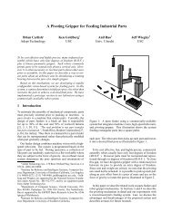
“Are We There Yet?” 11 Fig. 4. Probabilistic Foreground Segmentation and Tracking Pipeline. Upper Left: Raw image. Lower Left: Posterior probability image. Lower Right: Filtered and thresholded posterior image. Upper right: Bounding boxes of tracked foreground objects and annotated confidence levels. unique color. We define a lifting operation L : C → F ⊂ Rq3 by generating a unit vector on the axis corresponding to the input color. The set F is the “feature set,” representing all unit vectors in Rq3. Let fij(k) = L( Îij(k)) ∈ F be a feature (pixel color) observed at time k. Of the T observed features, select the Ftot ≤ Fmax most recently observed unique features; let I ⊂ {1, 2, . . . T }, where |I| = Ftot, be the corresponding time index set. (If T > Fmax, it is possible that Ftot, the number of distinct features observed, exceeds the limit Fmax. In that case, we throw away the oldest observations so Ftot ≤ Fmax.) Then, we calculate an average to generate the initial histogram: ˆ Hij(T ) = 1 Ftot r∈I fij(r). This puts equal weight, 1/Ftot, in Ftot unique bins of the histogram. 2.3 Bayesian Inference We use Bayes’ Rule to calculate the likelihood of a pixel being classified as foreground (F) or background (B) given the observed feature, fij(k). To simplify notation, let p(F |f) represent the probability that pixel (i, j) is classified as foreground at time k given feature fij(k). Using Bayes’ rule and the law of total probability,
Page 1 and 2: “Are We There Yet?” Visual Trac
Page 3 and 4: “Are We There Yet?” 3 people of
Page 5 and 6: “Are We There Yet?” 5 The opera
Page 7 and 8: “Are We There Yet?” 7 of the ba
Page 9: 1.6 Assumptions With this notation,
Page 13 and 14: “Are We There Yet?” 13 of pixel
Page 15 and 16: “Are We There Yet?” 15 vector,
Page 17 and 18: “Are We There Yet?” 17 and heig
Page 19 and 20: F2 Score F2 Score F2 Score 1.0 0.8
Page 21 and 22: 6 Acknowledgements “Are We There
Page 23 and 24: “Are We There Yet?” 23 14. Than
Page 25: “Are We There Yet?” 25 48. Emil

“Are We There Yet?” Visual Tracking of Visitors ... - Ken Goldberg

You also want an ePaper? Increase the reach of your titles

Delete template?

Save as template?