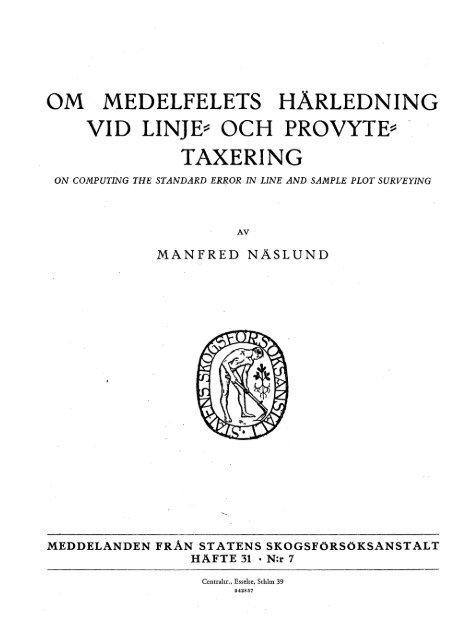
OM MEDELFELETs HÄRLEDNING VID LINJE::: OCH PROVYTE::: - TAXERING

OM MEDELFELETs HÄRLEDNING
VID LINJE::: OCH PROVYTE::: -
TAXERING
ON COMPUTING THE STANDARD ERROR IN LINE AND SAMPLE PLOT SURVEYING
AV
MANFRED NASLUND
MEDDELANDEN FRÅN STATENS SKOGSFöRSöKSANSTALT
HÄFTE 31 • N:r 7
Centraltr., Esselte, Sthlm 39
9428 57

MEDDELANDEN
FRÅN
STATENS
SKOGSFORSOKSANSTALT
MITTElLUNGEN AUS DER
FORSTLICHEN VERSUCHS­
ANST AL T SCHWEDENS
3l. HEFT
HÄFTE 3 I. I 938-39
REPOR TS OF THE SWEDISH
INSTITUTE OF EXPERIMENT AL
FORESTRY
N:o 31
BULLETIN DE L'INSTITUT D'EXPERIMENT A TIO N
FORESTIERE DE SUEDE
N:o 31
CENTRALTRYCKERIET, ESSELTE, STOCKHOLM 1939

REDAKTÖR:
PROFESSOR DR HENRIK HESSELlVIAN

INNEHÅLL:
Sid.
HESSELMAN, HENRIK: Fortsatta studier över tallens och granens
fröspridning samt kalhyggets besåning .................. .
W eitere Studien ii ber die Beziehung zwischen der Samenproduktion
der Kiefer und Fichte und der Besamung der Kahlhiebe. . . . . . . . 58
PETRINI, SvEN: Boniteringstabeller för bok. . . . . . . . . . . . . . . . . . . . . 6 5
Bonitierungstilfeln flir schwedische Buchenbestände . . . . . . . . . . . . . 8 5
FoRssLUND, KARL-HERMAN: Bidrag till kännedomen om djurlivets
i marken inverkan på markomvandlingen. I. Om några hornkvalsters
(Oribatiders) nåring . . . . . . . . . . . . . . . . . . . . . . . . . . . .
Beiträge zur Kenntnis der Einwirkung der bodenbewohnenden Tiere
auf die Zersetzung des Bodens I. Uber die Nahrung einiger Horn­
87
milbe (Oribatei). . . . . . . . . . . . . . . . . . . . . . . . . . . . . . . . . . . . . . . . . .
Redogörelse för verksamheten vid Statens skogsförsöksanstalt
under tiden 1932-3'/w 1937 jämte förslag till arbetsuppgifter
under den kommande femårsperioden. (Bericht Liber die
Tätigkeit der Forstlichen Versuchsanstalt Schwedens während der
Periode I932- 31. 10. 1937 nebst Vorschlag zum Arbeitsplan flir
die komroende Flinfjahrperiode; Account of the work at the Swedish
Institute of Experimental Farestry in the Period I 93 2- 3' j 10
I 93 7, with a Program for the work during the next five-year period)
I. Gemensamma angelägenheter (Gemeinsame Angelegenhei-
99
ten; Common topics) av HENRIK HESSELMAN ............... Io9
II. skogsavdelningen (Forstliche Abteilung; Farestry division)
av HENRIK PETTERSON. . . . . . . . . . . . . . . . . . . . . . . . . . . . . . . . . I lO
III. Naturvetenskapliga avdelningen (Naturwissenschaftliche
Abteilung; Botanical-Geological division) av HENRIK HEssEL-
MAN . . . . . . . . . . . . . . . . . . . . . . . . . . . . . . . . . . . . . . . . . . . I 2 o, 16 2
IV. skogsentomologiska avdelningen (Forstentomologische
Abteilung; EntomologicaJ division) av IvAR TRÄGÅRDH ...... IJ3
V. Avdelningen för föryngringsförsök i Norrland (Abteilung
flir Verjlingungsversuche in Norrland; Division for Afforestation
in Norrland) av EDVARD WIBECK ................... I 54
Utkast till program för studiet av skogsträdens raser vid Statens
skogsförsöksanstalt (Entwurf eines Arbeitsplans ftir das Studium
der Waldbaumrassen an der Forstlichen Versnchsanstalt Schwedens)
av HENRIK HESSELMAN ....................... , ..... I 58
HESSELMAN, HENRIK: Den naturvetenskapliga avdelningens verk=
samhet under åren 1902--1938 och avdelningens framtida
uppgifter. (Die Tätigkeit der Naturwissenschaftlichen Abteilung
während der Jahre 1932-1938 und deren zuktinftige Aufgaben) 163
MALl\ISTRöM, CARL: Hallands skogar under de senaste 300 åren.
En översikt över deras utbredning och sammansättning enligt officiella
dokuments vittnesbörd . . . . . . . . . . . . . . . . . . . . . . . . . . . . . . . 1 7 r
Die Wälder Hallands während der letzten 3oo J ah re. Eine Ubersicht
tiber deren Verbreitung und Zusammensetzung nach amtlichen
Angaben .................................. :. . . . . . . . . . . . 2 7 8

IV
N ÄSLUND, MANFRED: Om medelfelets härledning vid linje= och
provytetaxering . . . . . . . . . . . . . . . . . . . . . . . . . . . . . . . . . . . . . . . . 3 o I
On computing the standard error in line and sample plot surveying
................................................. 332
Redogörelse för verksamheten vid Statens skogsförsöksanstalt
under år 1937. (Bericht ii ber die Tätigkeit der Forstlichen Versuchsanstalt
Schwedens im Jahre 1937; Report on the work of the
Swedish Institute of Experimental Forestry in I 93 7)
Allmän redogörelse av HENRIK HESSELMAN ................. 345
L skogsavdelningen (Forstliche Abteilung; Forestry division)
av HENRIK PETTERSON ................................. 346
Il. Naturvetenskapliga avdelningen (Naturwissenschaftliche
Abteilung; Botanical-Geological division) a v HENRIK HEssELMAN 3 5o
III. skogsentomologiska avdelningen (Forstentomologische
. Abteilung; Entomological division) av IvAR TRÄGÄRDH ...... 353
Redogörelse för verksamheten vid Statens skogsförsöksanstalt
under år 1938. (Bericht tiber die Tätigkeit der Forstlichen Versuchsanstalt
Schwedens im Jahre I938; Report on the work of the
Swedish Institute of Experimental Forestry in I 938)
Allmän ·redogörelse av HENRIK HESSELMAN ........ ; ........ 355
l. skogsavdelningen (Forstliche Abteilung; Forestry division)
av HENRIK PETTERSON ................................. 355
II. Naturvetenskaplig-a avdeln1ngen (Naturwis

==M=A=N=F=. R=E=D=N=Ä=S=L=U=N=D==(!) .
OM MEDELFELETs HÄRLEDNING
VID LINJE- OCH PROVYTET AXERING.
Inledning.
Sedan vid värmlandstaxeringen den tanken blivit väckt att använda
sannolikhetskalkylens hjälpmedel för bestämningen av noggrannheten
hos en objektiv taxering (Kommisst:onen för försökstaxering etc. 1914),
ha ett flertal metoder för härledning av en taxerings medelfel framlagts.
Tillförlitliga sådana beräkningsmetoder utgöra en viktig förutsättning för
en rationell planläggning av våra skogstaxeringar. De framkomna metoderria
ha tidigare underkastats kritiska granskningar (LINDEBERG 1923, 1926,
LANGSARTER 1926, 1927, 1932, NÄsLUND 1930), varav bL a. framgått, att
ett starkt behov. av metodikens vidare utveckling förelåg. Avsikten är här
att lämna ett bidrag till denna fråga, som i samband med de förnyade riksskogstaxeringarna
i de nordiska länderna erhållit ökad aktualitet.
Den tidigare diskussionen av metodiken har huvudsakligen skett i anslutning
tilllinjetaxeringen, men vi skola nu även beröra metodfrågan för den
regelbundna provytetaxeringen, som tilldragit sig ett stort intresse, och för
vars objektiva bedömande en tillfredsställande metod vid medelfelets beräkning
erfordras.
Den i det efterföljande framlagda metoden för medelfelets härledning har
använts av mig vid vissa utredningar på uppdrag av I937 års riksskogstaxeringsnämnd.
Med nämndens benägna tillstånd illustreras framställningen av
exempel hämtade från denna undersökning. För detta tillmötesgående ber
jag att få uttala mitt tack.
Jägmästare E. ÖsTLIN har omhänderhaft den närmaste ledningen av det
omfattande räknearbetet för nämndens räkning, och förste skogsbiträdet
K. SVENSON har utfört räknearbetet vid det förberedande metodstudiet. Till
dessa medhjälpare vill jag rikta ett hjärtligt tack.
22. Meddel. från Statens Skogstörsöksanstalt. Häft. 3I.

302 MANFRED NÄSLUND
KAP. L DEN SENASTE UTVECKLINGEN AV METO­
DIKEN VID MEDELFELETs HÄRLEDNING.
Vi skola här endast uppehålla oss vid den utveckling, föreliggande fråga
haft, sedan jag förra gången behandlade detta ämne (NÄsLUND r930).
LANGSARTER har utfört en omfattande undersökning, vars syfte varit att
genom bearbetning av empiriskt taxeringsmateriallämna ett bidrag till frågan
om den noggrannhet, som uppnås vid linjetaxering av skogar av olika
storlek och sammansättning med användande av olika taxeringsprocenter
(LANGSAETER r932). I denna avhandling diskuterar LANGSARTER åter ingående
metodiken vid medelfelets härledning.
LANGsAETER framlägger i avhandlingens teoretiska del bl. a. en ny metod
för medelfelets beräkning (LANGSAETER r932, s. 46r, formel 2r). I denna formel
ingå differenser av den observerade storheten för linjeavstånd ända ned
..
till ro m. Utan ett extrapoleringsförfarande kan formeln ej användas i praktiken,
och som stöd för denna extrapolering saknas ett entydigt, funktionellt
samband. Metoden har därför huvudsakligen ett teoretiskt intresse, vilket
LANGSARTER själv framhåller.
X samband med en allmän prövning av de vanligaste formlerna för medelfelets
beräkning behandlar LANGsAETER även en av mig framlagd metod
(jfr NÄsLUND r930, s. 330, metod D: 2). Vid tillämpningen av densamma använder
LANGsAETER delvis ett annat förfaringssätt, än det jag anvisat. Tillvägagångssättet
överensstämmer ej med den ursprungliga tankegång, varpå
metoden vilar. J ag skall därför något uppehålla mig härvid.
Medeldifferensens utjämning avser i princip endast att eliminera den genomsnittliga
effekten av en ev. systematisk variation (tendens) från linje tilllinje
hos den taxerade storheten. Någon annan innebörd har ej givits åt differenskurvans
extrapolering till noll. Till grund för utjämningen .skall därför endast
läggas de medeldifferenser, som kunna bildas av i taxeringen ingående linjer.
När LANGSARTER för mycket lågprocentiga taxeringar härleder den aktuella
taxeringens medeldifferens med ledning av medeldifferenserna för ro och
20 m:slinjeavstånd, innebär detta i princip något helt annat och tyder på en
felaktig tolkning av metodens teoretiska underlag (LANGSAETER r932, s. 483).
För vissa jämförelser har jag (NÄsLUND r930, tab. II, s. 335) beräknat soch
2Y2-procents taxeringarnas medelfel med stöd av ro-procents taxeringens
medeldifferens. Detta är emellertid ej någon tillämpning av metoden utan ett
approximationsförfarande, som tillgripits i brist på andra utvägar och har
karaktären av en relativt måttlig extrapolering.
LANGsAETER visar vidare, att min metod under vissa förutsättningar ger
samma resultat som hans metod C: 2 (jfr LANGsAETER r932, s. 47r), vilken

MEDELFELET VID LINJE- OCH PROVYTETAXERING 305
serna (x,- M) fördela sig enligt den normala sannolikhetsfunktionen (HEL­
MERT I9Z4, s. 75). Medelfelets relativa medelfel vid olika gruppantal (n)
framgår av nedanstående sammanställning:
n= 2 3 4 5 6 7 8 9
SsM=J0,7 o/o, 50,o %. 40,8 %. 35.4 %. 3I,6 %, z8,9 %. z6,7 %. Z5,o %.
n= ro 15 20 25 30 40 so
SsM=Z3,6 %, I8,9 %, I6,2 %, I4,4 %, I3,I %, II,3 %, IO,r %·
Osäkerheten i de beräknade medelfelen är betydande för de gruppantal,
som hittills vanligen kommit till användning (8-zo st.). Gäller det att beräkna
medelfelet för en enskild taxering, måste denna således uppdelas i ett
re_lativt stort antal deltaxeringar (grupper). Här komma vi till en allvarlig
begränsning hos metod A.
Vid en uppdelning av taxeringen i ett större antal grupperriskerar man ofta,
såvida antalet linjer eller delsträckor ej är mycket stort, att en systematisk
gång gör sig gällande i gruppresultaten (jfr LANGSARTER Igz6,
NÄsLUND I930). Under sådana förhållanden ger formel (I) för höga medelfeL
Minskningen av det tillfälliga felet köpes sålunda med ökad risk för systematiskt
fel.
Det systematiska felet kan emellertid nedbringas genom att på deltaxeringarna
tillämpa formel (z), men inflytandet av den systematiska gången
från grupp till grupp kvarstår alltid. Risken för ovannämnda systematiska
tendens är dock betydligt mindre, om taxeringslinjerna uppdelas i delsträckor,
som kombineras efter ett visst system (jfr NÄsLUND I930, metod A: z, s.
3ZI). Bortsett från ovannämnda risk för ett systematiskt för högt medelfel
är metoden även ur en annan synpunkt otillfredsställande.
Gemensamt för metod A är, att man ur deltaxeringarnas medelavvikelse
beräknar den aktuella taxeringens medelfel (sM). En sådan extrapolation
stöter alltid på svårigheter och måste betraktas som en svaghet hos metoden.
Vi återkomma härtill i det efterföljande (s. 3I5).
M e t o d C torde ha framtvingats av behovet att vid metod A uppdela den
aktuella taxeringen i ett flertal deltaxeringar. De i en taxering ingående linjerna
uppgå nämligen ej sällan till ett så ringa antal, att man ej ens kan uppdela
dem i ett mindre antal deltaxeringar.
För metod C och formel (z) kan medelfelets relativa medelfel vid ett linjeantal
av omkring IO och däröver approximativt uppskattas till samma storlek
som för metod A och formel (I), varvid n (formel 3) nu betyder antalet
taxeringslinjer. Metod C lämnar därför ofta ett med hänsyn till de tillfälliga
felen relativt säkert medelfeL För taxeringar av småskogar föreligger dock

306 MANFRED NÄSLUND
ett behov att kunna dela upp taxeringslinjerna i mindre enheter (jfr s. 320).
Metoden har emellertid en annan svaghet.
I regel kan man spåra en systematisk gång i taxeringsresultaten för de enskilda
linjerna (LANGSAETER I926, NÄsLUND I930, ÖsTLIND I932, jfr även
fig. I-6, s. 308-I3). Under sådana förhållanden ger formel(2) för högt resultat,
emedan den systematiska tendensen från linje till linje ej bortelimineras.
Enligt ÖsTLIND torde formel (2) beträffande kubikmassan per hektar skogsproduktiv
mark i genomsnitt ge omkring 20 procent för stora medelfel
(Riksskogstaxeringsnämnden I932, ÖsTLIND I932). LANGsAETER uppskattar
detta systematiska fel till IO a 20 procent (Landsskogtakseringen I938).
För vissa behov kan man givetvis bortse ifrån en överskattning av denna
storleksordning och nöja sig med att vara på den säkra sidan. Gäller det däremot
att beräkna medelfelet på skillnaden mellan två taxeringsresultat,
vilket f. n. i samband med den förnyade riksskogstaxeringen är en aktuell
fråga, ökas kravet på bestämningen av den enskilda taxeringens medelfeL
Vi skola närmare· exemplifiera detta.
Antaga vi, att exempelvis virkesförrådet vid första taxeringen är M och
vid den andra k· M, samt medelfelet vid båda uppskattningarna s M procent,
erhålles ett enkelt uttryck för differensens relativa medelfel (sD). Härvid
skilja vi på om förrådet minskar eller ökar.
k I l I,5 l z
Il
Tab. I. Medelfelet på differenser (BD).
The standard error of differences.
l
l
B M i procent.
in percentage.
2,5 ! 3 l 3,5 l 4 l 4,5 l 5
BD i procent. Minskning.
in percentage. Decrease.
o,9
0,8
I3,4
6,4
zo,z
9,6
z6,9
IZ,8
33,6
r6,o
40,4 47,I
Ig,z l 22,4
53,8
25,6
6o,5
z8,8
67,3
32,o
0,7 4,I 6,r 8,r ro, z I Z, z I4,2 I6,3 I8,3 20,3
o,6
0,5
2,9
z,z
4,4
3,4
5,8
4,5
7,3
5,6
8,8
6,7
ro,z
7,8
II,7
g,o
I3,2
ro, r
I4,6
II,2
s D i procent. Ökning.
in percentage. Increase.
I, I
I,z
I4,9
7,8
22,3
II,7
29,7
I5,6 19,5
5Z,o
23,4 27,3
59,5
31,2
66,9
35,I
74,3
39,0
1,3 5,5 8,z 10,9 13,7 I6,4 rg,r 21,9 24,6 27,3
1,4
I,5
4,3
3,6
6,4
5,4
8,6
7,2
ro,B
9,o
12,9
ro,B
15,I
12,6
17,2
14,4
19,4
16,2
21,5
18,o
l 37,2 44,6 l
l
l
l
l

MEDELFELET VID LINJE- OCH PROVYTETAXERING 307
Virkesförrådet minskar (k< r):
Virkesförrådet ökar (k> r):
SM VI+ k 2
SD = I -k ' . . . . . . . . . . . . . . . . . . . . (4)
SM VI+ k2
sn = k- I ' . . . . . . . . . . . . . . . . . . . . (S)
där sn och sM äro uttryckta i procent.
Formlerna (4) och (5) ha tabellerats för vissa värden på k och sM (tab. r).
Härav framgår med skärpa svårigheten att uppskatta små förändringar
samt betydelsen av en god bestämning av de enskilda
taxeringarnas medelfeL
Den förda diskussionen torde ha visat, att man vid ett sökande
efter en lämplig metod för medelfelets härledning måste
uppställa som krav, att medelfelets såväl systematiska som
tillfälliga fel vid behov skola kunna nedbringas så långt
som möjligt.
KAP. III. TEORI OCH METODIK.
Linjetaxering.
De svårigheter, som äro förbundna med beräkningen av medelfelet för en
regelbunden linje- eller provytetaxering, bero huvudsakligen på att taxeringslinjerna
utläggas systematiskt och ej uttagas på slump. När linjeriktningen,
taxeringsprocenten och läget av första taxeringslinjen bestämts, är även belägenheten
av de övriga taxeringslinjerna angiven. Linjernas systematiska
utläggande sker uppenbarligen i syfte att öka taxeringsresultatens säkerhet.
Att så även är fallet framgår av ÖsTLINDs ovannämnda utredning (ÖsTLIND
1932, S. 451).
Det har tidigare framhållits, att taxeringsresultatet ofta varierar systematiskt
från linje tilllinje (jfr. s. 306), och vi skola här i några exempel närmare
analysera taxeringens struktur. För detta syfte har valts förra riksskogstaxeringen
av Västernorrlands och Norrbottens län, vilka ur taxeringssynpunkt
representera olika svårighetsgrader.
Vid riksskogstaxeringen ha taxeringslinjerna indelats i 2 km långa sträckor.
Denna indelning är utförd så, att sträckor med samma z-km nummer bilda
ett mot taxeringsriktningen vinkelrätt fält (block). I det efterföljande äro zkmna
sammanslagna till r-mil sträckor. För r-mil sträckor med samma nummer
införa vi benämningen taxeringsblock eller enbart block.

MEDELFELET VID LINJE- OCH PROVYTETAXERING 315
Kubikmassan inom bark per hektar landareal (Västernorrland) eller landareal
exkl. inägor (Norrbotten) har uträknats för varje linje och block inom de båda
länen, varvid Norrbotten uppdelats på kustland och lappmark. Kubikmassan
har redovisats på tall och gran samt dimensionsgrupperna: I5 cm vid brösthöj d
och däröver, 25 cm och däröver samt 35 cm och däröver. I fig. I-6 har kubi.}{massan
per hektar upplagts grafiskt med linje-, resp. blocknumret som oberoende
variabel. Linjerna äro numrerade från sydost till nordväst och blocken
från sydväst till nordost. Linjeavståndet utgör för Västernorrlands län en
mil och för Norrbottens två mil.
Figurerna visa tydligt, att för såväl linjer som block en markerad
systematisk gång ofta gör sig gällande i taxeringsresultaten.
Denna tendens är ej sällan mycket starkt utpräglad. Härtill bidrar
givetvis att tallens och granens kubikmassor angivits skilda åt, vilket är motiverat
därav, att det föreligger ett behov att kunna beräkna säkerheten hos
dessa uppskattningar var för sig.
Beträffande arealbestämningar har LANGSARTER påvisat samma tendenser
(LANGSAETER I926).
För Norrbottens lappmark har i fig. 7 fördelningen av granens kubikmassa
över I5 cm närmare åskådliggjorts med ledning av taxeringsresultaten från
I-mil sträckorna. Av figuren framgår, att kubikmassan å en lin j esträcka
i viss grad är en funktion av sträckans avstånd till
två koordinataxlar. Det är uppenbart, att vid medelfelsmetodikens
utformning stor hänsyn måste tagas till förekomsten ·
a v här illustrerade fördelnings tendenser.
Innan vi övergå till att diskutera medelfelsberäkningens teori, skola vi något
dröj.a vid de metoder, som grunda sig på att taxeringslinjerna eller delar
därav sammanföras i grupper (jfr NÄsLUND I930, metod A: I och 2).
Vi förutsätta, att den utförda linjetaxeringen är en IO-procents taxering,
och att den är uppdelad i IO grupper, som var och en omfattar en I-procents
taxering. Det efter denna metod beräknade medelfelet är då approximativt
det riktiga medelfelet för den taxering, som erhålles, om man av de IOO stycken
möjliga I-procents taxeringarna av skogen på slump plockar ut IOstycken
och därav bildar en IO-procents taxering (jfr LANGSARTER I932, s. 446).
Det är emellertid ej detta medelfel, vi önska veta, utan medelfelet på
den systematiskt utlagda Io-procentiga linjetaxeringen.
Med taxeringslinjernas systematiska utläggande avses, att varje linje eller
del därav (exv. I-mil sträcka) skall representera den parcell av skogen, som
ligger inom halva Jinjeavståndet på vardera sidan om linjen (delsträckan).
Kände vi resultatet (xi) av en totaltaxering för varje sådan avdelning, skulle
linjetaxeringens medelfel (eM) erhållas enligt formlerna:

MEDELFELET VID LINJE- OCH PROVYTETAXERING 321
Vid den regelbundna provytetaxeringen göres i regel den enskilda provytan
relativt liten, för att den endast i undantagsfall skall behöva fördelas på olika
markslag eller andra arealbestämningar. Det på sina håll tillämpade
förfaringssättet att i sådana fall flytta ytan, så att den endast
omfattar ett markslag, är ur statistisk synpunkt oriktigt och
bör ej komma till an vändning. Under ovan nämnda förutsättningar
blir variationen i princip alternativ, d. v. s. antingen finns egenskapen
å ytan, eller också finns den ej. Det ligger då nära till hands att söka härleda
arealbestämningarnas medelfel med stöd av den alternativa eller
homograda statistikens klassiska satser.
Sådana försök ha gjorts av ScHUMACHER och BULL (1932) samt av Mun­
GETT och GEVORKIANTZ (1934). Härvid har principiellt hela taxeringen hänförts
till ett visst urnschema, varvid de förra tillämpat BERNOULLis och de
senare POISSONS eller LEXIS schema (CHARLIER 1931). LANGsAETER har visat,
att fördelningen av olika markslag har samma tendenser, som vi här funnit
hos kubikmassan (jfr. s. 315). Det är för övrigt helt naturligt, att så skall vara
fallet. En tillämpning av det enklaste urnschemat (BERNOULLis) på hela
taxeringsobjektet måste därför betraktas som alltför schematisk, vilket även
framgått av de ovannämnda undersökningarna. MunGETTs och GEVORKI4NTZs
användning av PolsSONs eller LEXIS teorem är därför en utveckling i rätt
riktning mot verklighetens komplexa urnschemata.
En närmare anpassning av beräkningsmetodiken till de faktiska förhållandena
kan ske på två sätt. Antingen genom kombinationer av PolssoNs
och LEXIS schemata eller också genom uppdelning av taxeringen i mindre
enheter, för vilka BERNOULLIS schema approximativt är tillämpligt. J ag har
i anslutning till metodiken för härledningen av kubikmassans medelfel valt
den senare vägen.
Vi återvända till den i det föregående (s. 316) använda indelningen av skogen
i rutor. Dessa rutor betrakta vi som urnor med approximativt regellöst (slumpvis)
fördelade svarta och vita kulor. Kulorna utgöras av de provytor, vari
den enskilda rutan kan tänkas uppdelad. Härvid betecknar exv. de svarta
kulorna det markslag, vars medelfel skall härledas. Taxeringen av rutan sker
visserligen strängt systematiskt, emedan provytorna utläggas i ett visst förband.
Men om arealens fördelning inom rutan ej visar några systematiska
tendenser, kunna vi approximativt betrakta provytetaxeringen som dragningar
ur en urna, varvid delJ. för varje gång dragna kulan ej lägges tillbaka i
urnan. Antalet dragningar motsvaras härvid av antalet provytor, som vid
taxeringen utfalla i rutan. Under sådana förutsättningar kan provytetaxeringens
medelfel för den enskilda rutan lätt beräknas.
Låt N beteckna totala antalet provytor, vari i:te rutan kan tänkas uppdelad
(rutans areal: provytans areal) och p, antalet vid taxeringen utfallande

l
326 MANFRED N ÄSLUND
Norrbottens lappmark ................
Norrbottens kustland ................
Västernorrlands län ...................
l Tall
Pin e
Gran
Spruce
Tall
Pin e
Gran
Spruce
Tall
Pin e
Gran
Spruce
Tall
Ljungans flodområde : Västernorrlans- Pin e
delen • o ••• o. o o •••••••••••••••••• o Gran
Spruce
Ljungans flodområde:
l Tall
Jämtlandsdelen
Hela Ljungans flodområde ............
Medeltal -
Avetage
Pin e
Gran
Spruce
Tall
· Pine
Gran
Spruce
l
Tab. 4· Medelfelet å kubikmassan per hektar
The standard error of cubic vollime per hectare
15-
'•
Dimensions-
Diameter-
Taxeringsområde
Survey district
Medelfel i procent
standard ettor in percentage
Trädslag
Tree species å taxeringsresultatet vid taxenligt
ering av
The actual survey roohektar
accord. to enligt forme!
12
Surveying
formel 121 formel 14 Ioo hectares
farmula 12 farmula 14 accord. to
farmula 12
Kol. 4
i %
av
kol. 3
Col. 4
in o/0
of
col. 3
Kubik-
massa
per ha
Cubic
volume
per
hectare
I l 2 l 3 l 4 l 5 l 6 l 7
4,15 5,34 18,2 129 ro, 58
5,54 6,o7 24,3 110 6,r5
3,28 4,21 11,5 128 13,77
7,28 7,69 25,6 106 6,55
3,17 3,63 15,5 115 10,32
2,65 3,08 13,0 116 15,64
5>3 I 6,53 11,9 123 13,20
5,4I 5,97 I2,I 110 18,o7
5,73 5,77 14,1 101 13,35
5,99 7,46 14,7 125 14,31
3,96 - 13,2 - 13,28
4,02 - i:3,4 - 16,o2
-
l -
l -
l 116
l -

med hänsyn till grundytans osäkerhet.
accord. to uncertainly of the basal area.
grupp
dass
MEDELFELET VID LINJE- OCH PROVYTETAXERING 327
25-
Medelfel i procent
standard error in percentage
Kol. 9
å taxeringsresultatet vid tax- i%
enligt ering av av
The actual survey Joohektar kol. 8
accord. to enligt for- Col. 9
mel 12 in%
of
Surveying col. 8
formel 121 formel I4 roo hectares
formuta u formuta r4 accord. to
tormula 12
8 l 9 l JO l II
4,41 5,46 19,3 124
7,o6 7,46 30,9 106
5,55 6,17 19,5 III
11,55 I2,IO 40,6 105
4,29 4,74 2I,o IIO
4,15 4,62 20,3 III
7,r8· 8,34 16,1 II6
9,22 9,58 20,6 104
7,16 7,22 17,6 101
8,27 II,OI 20,3 133
5,Io - 16,9 -
6,r9 - 20,6 -
-
l -
l -
l 112
Kubikmassa
per ha
Cubic
volume
per
hedare
l 12.
5,81
2,67
5,27
1,79
4,71
4,04
6,24
5,06
6,47
4,24
6,37
4,61
l -·
35-
Medelfel i procent
standard error in percentage
å taxeringsresultatet vid taxenligt
ering av
The actual survey Joohektar
accord. to enligt formel
12
Surveying
formel 121 formel r4 roo hectares
l tormula u tormula 14 accord. to
tormula u
Kol. 14
i %
av
kol. 13
Col. r4
in%
of
col. r3
Kubik-
massa
per ha
Cubic
volume
per
hectare
Il
Il 13 l 14 l 15 l !6 l 17
6,77 7,04 29,6 104 1,6 I
8,95 9,82 39,2 IIO 0,73
8,92 10,78 31,4 121 0,79
17,63 18,oo 61,9 102 0,25
6,8o 7,43 33,3 109 1,02
7,72 8,29 37,8 107 0,53
9,75 12,05 21,8 124 1,54
14,30 ):5,38 32,0 108 o,B2
12,I4 12,12 29,8 IOO 1,37
14,"6o 16,65 35,8 II4 0,55
7,83 - 26,o - 1,45
10,30 - 34·2 - o,67
-
l -
l -
l
Il O
-
l -

328 MANFRED NÄSLUND
Tab. 5· Jämförelse mellan enligt formel (2) och enligt formel (12) beräknade medelfel.
Comparison between standard error computed accord. to formula (z) and formuta (Iz).
Antal Medelfel i pro- Kol. 6
Number of cent enligt
Dimen-
i %
Trädstandard
error in
Taxeringsområde sions
av
tax- slag percentage accord. to
kol. 7
Survey district eringsgrupp
rutor Tre e
Diam.-
Col. 6
linjer
species
squares
el ass in%
formel 21formel I 2
survey
of
lin e s formuta z formuta rz col. 7
I l 2 l 3 l 4 l 5 l 6 l 7 l 8
Norrbottens lappmark l II 225
Tall r l s- 3,77 4,r5 gr
Pin e 25- 5,84 4,4I .r32
l
35- 8,68 6,77 !28
l
Gran r s- 5,r I 5,5 4 92
Spruce z s- 5,8 I 7,o6 82
35- 8,44 8,95 94
l
Norrbottens kustland:
l
r2 r62
Tall
Pin e
Gran
Spruce
ISz
s--
35r
s-
z s·-
5,43
7,85
13,34
8,96
I2,5 7
3,28
5,55
8,92
7,28
I r,5 5
r66
I4r
!50
r23
I09
35- 23,03 !7,63 I3r
l
Tall r s- 3,I9 3,I7 IOI
I,ine 25- 3,34 4,29 78
l
35- 6,77 6,8o IOO
Västernorrlands län . "l 27 29I ' Gran IS- 3,I9 2,65 I20
l
Spruce 25- 4,37 4,I5 ros
. 35- 8,77 7,72 II4
l
Medeltal -
Average
l
-
l II4
KAP. IV. OM V ALET A V METOD FÖR MEDELFELETs
HÄRLEDNING.
Vid valet av metod för medelfelets härledning gäller den allmänna regeln
att anpassa metoden efter det föreliggande behovet. I vissa fall är det nödvändigt
att arbeta med den största noggrannhet, som kan åstadkommas,
i andra fall äro enklare metoder fullt tillfredsställande, varför de för kostnadernas
nedbringande böra äga företräde.
Det är givetvis omöjligt att ange några generella regler, när den ena eller
andra metoden bör användas. Detta beror dels på det behov, medelfelsberäkningen
skall tillfredsställa, dels på taxeringsmaterialets inre struktur. Vi
kunna därför endast anlägga några allmänna synpunkter på frågan. Härvid
behandla vi linje- och provytetaxeringen var för sig.

330 MANFRED NÄSLUND.
KAP. v. SAMMANFATTNING.
Vid sannolikhetskalkylens tillämpning på praktiska frågeställningar är
det ofta svårt att bevisa tillämpningens berättigande. Sannolikhetskalkylen
i här avsedd bemärkelse vilar på rent matematisk grund och bygger således
på vissa bestämda förutsättningar, som endast med större eller
mindre approximation kunna återfinnas i ett konkret material. Graden av
approximation blir avgörande för kalkylens värde. För sannolikhetskalkylens
praktiska användning är det således av väsentlig betydelse, att tillämpningsmetoder
utvecklas, som ej bygga på några speciella förutsättningar
utan endast på mera allmängiltiga sådana. Varje framträngande mot detta
mål måste betraktas som ett framsteg.
Avsikten med denna uppsats har varit att lämna ett bidrag till en sådan
utveckling av metodiken för medelfelets härledning vid linje- och provytetaxering.
Den här framlagda huvudmetoden (formel 12, s. 317) innebär
ett nytt grepp på denna fråga och gäller i princip även om
systematiska tendenser· föreligga med avseende på taxeringsobjektets
fördelning, vilket är ett ofta förekommande fall.
Metoden har använts av mig för beräkningen av medelfelet å virkesförrådet
vid den förra riksskogstaxeringen av Västernorrlands och Norrbottens län
samt Ljungans flodområde (tab. 4, s. 326). Denna bearbetning utgör ett
empiriskt material av'betydande värde för belysandet av linjetaxeringens
noggrannhet. Undersökningen har dock här endast utnyttjats
i syfte att jämföra olika metoder för medelfelets härledning, under det
att en mera taxatariskt betonad diskussion av detsamma ansetts falla utom
ramen för denna uppsats.
För härledning av medelfelet å arealbestämningar vid provytetaxering
har dessutom utvecklats en specialmetod (s. 322). Metoden
är föga arbetskrävande och synes ej sällan vara användbar.
Anförd litteratur.
BACHER, I., 1933, Moderna synpunkter på fältförsökets metodik och den statistiska
analysen av försöksresultatet. Nord. Jonfbr. Forskning.·
CHARLIER, c. v. L., 1931, Vorlesungen iiber die Grundziige der mathematischen statistik.
Lund.
CRAMER, HARALD, 1926;Sannölikhetskalkylen och några av dess användningar. Stockholm.
CzuBER, E., 1924, Wahrscheinlichkeitsrechnung. Erster Band. Leipzig und Berlin.
F1SHER, R. A., 1932. Statistical Methods for Research Workers. Edinburg.
HELMERT, F. R., r924, Die Ausgleichungsrechnung nach der Methode de:r kleinsten
Quadrate. Leipzig und Berlin.
HESSELMAN, H., 1935, Barrskogens arealfördelning på tall-, gran- och barrblandbestånd
i Norrland och Dalarna. Medd. från Statens skogsförsöksanstalt. H. 28, nr 8.

MEDELFELET VID LINJE- OCH PROVYTETAXERING 331
Kommissionen för försökstaxering etc., 1914, Värmlands läns skogar. Betänkande. Stockholm.
Landsskogtakseringen, 1938, Taksering av Norges skoger. 0stfold fylke. Oslo.
LANGSAETER, A., 1926 och 1927, Om beregning av middelfeilen ved regelmessige linjetakseringer.
Medd. fra det norske skogforsoksvesen, H. 7 och 8.
-- 1932, Noiaktigheten ved linjetaksering av skog I. Medd. fra det norske skogforsoksvesen,
H 15.
L1NDEBERG, J. W., 1923, Uber die Berechnung des Mittelfehlers des Resultates einer
Linientaxierung. Acta forestalia fennica, H: 25.
-- 1926, Zur Theorie der Linientaxierung. Acta forestaHa fennica, H. 3r.
MUDGETT, BRUCE D. and GEVORKIANTZ, S. R., 1934, Reliability of forest surveys. Journal
of the American Statistical Association.
Riksskogstaxeringsnämnden, 1932, Uppskattningen av Sveriges skogstillgångar verkställd
åren 1923-29. Stockholm. ·
SCHUMACHER, FRANCis X. and BULL, HENRY, 1932, Determination of the errors of estimate
of a forest survey, with special reference to the bottom-land hardwood forest
region. J our:nal of Agricultural Research.
SNEDECOR, GEORGE W., 1934, Calculation and interpretation of analysis of variance
and covariance. Ames. Iowa.
TIREN, LARS, 1934, Nyare fältförsöksmetodik, belyst genom några skogsodlingar på
Kulbäckslidens försökspark. Medd. från Statens skogsförsöksanstalt. H. 27, nr 6.
YULE, G. UDNY and KENDALL, M. G., 1937, An introduction to the theory of 'statistics
London.
ÖSTLIND, J. och HAGSTRÖM, H. G., 1922, Felrisken vid provtaxering (manuskript).
ÖsTLIND, J., 1932, Erforderlig taxeringsprocent vid linjetaxering av skog. Skogsvårdsför.
tidskrift.

332 MANFRED NÄSLUND
RESUME.
On computing the standard error in line and sample plot
surveying.
Introduction.
Since the Värmlandian survey has proved the application and suitability of
the probability-computation for determining the degree of accuracy in an objective
survey (the Commission for an experimental survey etc., 1914), several methods
have been suggested for computing the standard error in a survey. Reliable
methods of calculation of this kind are an important condition for planning our
forest sm:veys on rational lines. The methods proposed have previously been subjected
to critical scrutiny (LINDEBERG 1923, 1926, LANGSAETER 1926, 1927, 1932,
NÄsLUND 1930), which revealed, inter alia, the fact that it was highly necessary
to develop the methodics of the subject still further. The object here is to make
a contribution to this question, whkh has become an increasingly urgent one in
conjunction with the renewal of the national forest surveys in the Northern
Countries.
The method proposed in the following artide of computing the standard error
has been employed by me in certain inquiries made on behalf of The National
Forest Survey Commission of 1937.
The most recent development of the methods of computing the
standard error.
We shall here merely confine ourselves to the development which the question
under discussion has undergone since I last dealt with the subject (NÄsLUND 1930).
LANGsAETER has carried out a far-reaching investigation, the aim of which was
by compiling empirkal survey material to contribute towards solving the question
of what degree of accuracy is attairred in the linesurveying of forests of various
size and composition (evenness) with the use of different survey percentages
(LANGSAETER 1932). In this paper LANGSAETER again disensses at length the
methodks of computing the standard error.
In the theoretkal section of his paper LANGsAETER gives, among other things,
a new formula for calculating the standard error (LANGSAETER 1932, p. 461,
formula 21). Thisformula contains differences of the seeond order in the observed
quantity for distances between the lines right down to Io m. The formula cannot
be used without a process of extrapolation, and there is no definitly known function
in support of this extrapolation. The method is therefore, as LANGsAETER
himself points out, only of a certain theoretkal interest.
In making a general trial of the most common formulae for calculating the
mean error, LANGsAETER discusses, among others, a method suggested by me
(cf. NÄsLUND 1930, p. 330, method D: z). When employing it LANGsAETER uses,
in part, a method of procedure different from the one given by me. His procedure

MEDELFELET VID LINJE- OCH PROVYTETAXERING 333'
is not in accord with the original train of thought on which my method is based.
I shall therefore dwell on this point briefly here.
In principle, the purpose of smoothing out the mean difference is merely to
eliroinate the average effect of any systematic tendency there might be from
line to line in the actual survey. No other rueaning has been given to the extrapolation
of the difference-curve to zero. As the basis of the smoothing out process,
therefore, we shall only take those mean differences which may arise from lirres
included in the survey.
When for very low-percentage surveys LANGSAETER calculates the mean difference
of the actual survey with the guidance of the mean differences for ro and 20
m line distances, this implies in principle something quite different and indicates
an erroneous interpretation of the theoretical grounds on which the method is
based (LANGSAETER 1932, p. 483). For certain comparisons I have calculated
(NÄsLUND 1930, tab. II, p. 335) the 5 and 2 Yz % surveys' standard error on the
basis of the ro% survey's mean difference. This is however not an application
of the method but a process of approximation resorted to for lack of other means,
and has the charader of a relatively moderate extrapolation.
LANGsAETER further shows that under certain conditions my method gives
the same results as his method C: 2 (cf. LANGsAETER 1932, p. 471), which has the
advantage of requiring less labour. We need only add the observation tbat this
presupposes, inter alia, a smoOthing-out of the mean-difference curve with the
aid of only 2 points, which of course was not the intention (cf. NÄsLUND 1930,
p. 332, fig. 6).
The method discussed above has been proposed by me in connection with an
examination of the methodics used in computing the standarderror and was then
explanatory and of mainly theoretical interest. However, it has a limited practical
utility, as I have pointed out previously (NÄsLUND 1930, p. 330), sothat it is not
necessary to dwell on that point here.
In Sweden, ÖsTLIND has carried out a comprehensive investigation on behalf
of the Royal Board of Domains with the same object in view: as LANGSAETER's
above-mentioned enquiry (ÖsTLIND 1932). ÖsTLIND discusses here the theory
of computing the standard error in line surveying and deduces a formula for the
standard error, which formula may be regarding as a modification or variant of
LANGSAETER's formula based on differences of the seeond order (LANGSAETER
1926, 1927 and 1930).
In the U. S. A. an opportunity has been afforded by the regular sample
plot survey to make a close study of the object airned at here (ScHUMACHER
and BULL 1932, M UD GETT and GEVORKIANTZ 1934). For this purpose the question
of computing the standard error has been discussed in conjunction with the
theorem of BERNOULLIS, PorssoN and LEXI, to which we shall revert in p. 341.
In the following pages we shall call the regular sample plot survey merely the
sample plot survey, meaning thereby a survey consisting of a number of fairly
small sample plots in a certain regular formation.
The above observations cover the most important known works which have
been published since 1930 and deal with the question of the methodics used in
computing the standard error in regular line and sample plot surveying. It will
have been gathered that for calculating the standarderror in an actualline survey
we still have to take recourse to those methods which were employed when I
dealt with this subject in my former paper, to which the reader is referred in order
24· Meddel. från statens Skogsförsöksanstalt. Häfte 3I.

334 MANFRED NÄSLUND
to avoid unnecessary repetition (NÄsLUND 1930). On the other hand, our experiences
in regard to the accuracy of the line survey have become greatly widened as a
result of the considerable amount of work expended on compiling empirical survey
material (LANGSAETER 193z, ÖsTLIND 193Z, The National Forest Survey Commission
193z).
General views on the question of method.
Of the methods proposed there are principally two that in Sweden have been in
practical use for calculating the standard error in an actual survey. In my previous
paper on the subject these methods were denoted by method A. and method C.
respectively (NÄsLUND 1930), and theseletters willserve the same purpose in the
following discussion.
Method A. The survey lirres or parts thereof are divided into groups (partial
surveys), after which the standarderror (s M) is calculated accordingto the farmula
(r), p. 304, in which x.; denotes the survey results of the i-th group, p, its total
length of line and n the number of groups.
Method C. The standard error is calculated with the aid of differences
between the survey results derived from succeeding survey lines. Standard error
formulae according to this principle are given by ÖsTLIND-HAGSTRÖM (r9zz),
LINDEBERG (I9Z3, 19z6) and LANGSARTER (19Z4, 193Z). For this purpose LANG­
SAETER's farmula based on differences of the seeond order has often been preferred
(LANGSAETER r93Z, method C: z). The standard error is then obtained by
means of the following (z), p. 304, in which x.; is the result survey and P.; the
surveyed length for the i-th survey line, where i indicates the sequence of the
lines. n derrotes the number of survey lines.
Sametimes a earobination of these methods has been used, the lines being
first divided into groups and farmula (z) being then applied to the group results.
Taking these methods as oilr background we shall discuss in detail the problem
as it now presents itself.
The calculated standarderrors are in their turn liable to standarderrors owing
to the limited number of variants (partial surveys, survey lines, as the case ma y be).
By employing method A and farmula (r) the standard error in the standard
error can be obtained from farmula (3) p. 304 where n is the number of
groups. Formula (3) assumes tbat the deviations (xi-M) are distributed in accordance
with the normal function of prohability (HELMERT 19Z4, p. 75). The
relative standard error in the standard error (s, M) by using different numbers
of groups (n) will be seen from the table on p. 305.
The uncertainty in the calculated standard errors is considerable ·in the case
of those numbers of groups which have hitherto been customarily used (8-·zo).
If, then, the standard error is to be calculated for an individual survey, it must
be divided up into a relatively large number of partial surveys (groups). This
brings us to a serious limitation inherent in method A.
In dividing up the survey into a. considerable number of groups there is often
the risk, provided the mimber oflines is not very large, of a systema tic varia tio n
(tendency) appearing in the group results (cf. LANGSARTER 19z6, NÄsLUND 1930).
Under such circumstances farmula (r) produces too high standard errors. Consequently
the reduction of the accidental error is made at the east of an increased
risk of a systematic error.

MEDELFELET VID LINJE- OCH PROVYTETAXERING 335
The systematic error can however be reduced by applying formula (z) to the
partial surveys, but the influence of the systematic variation from group to group
is always present. Nevertheless the risk of a systematic variation, as mentioned
above, is far less if the survey lirres are divided up into partial sections, which are
combined according to a certain system (cf. NÄsLUND 1930, method A: z, p. 3zr).
Apart from the above-mentioned risk of a systematically too high standard error,
the method is also unsatisfactory from another point of view.
A common feature of method A is that the standard error (s M) of the actual
survey is calculated from the standard deviation of the partial surveys. Such an
extrapolation is invariably fraught with difficulties and must be regarded
as a weakness iu the method. We shall revert to this point later on.
Method C has apparently arisen out of the necessity, when applying method A,
for dividing up the actual survey into a number of partial surveys; for not infrequently
the lines included in a survey are so few in number that one cannot even
divide them up into a smaller number of partial surveys.
In respect of method C and f ormula (z) the relative standard error in the standard
error if the line-number is about ro and over can be approximately estimated at
the same size as in respect of method A and formula (r), n now meaning the number
of survey lines. Frequently, therefore, method C produces a standarderror which,
if account is taken of the accidental error, is relatively certain (cf. p. 305). In
surveying small forest areas, however, one must be able to divide up the survey
lines into smaller units (cf. p. 340). However, the method possesses a further
weakness.
It is generally possible to trace a systematic variation in the survey results of
the individual lirres (LANGSAETER 19z6, NÄsLUND 1930, ÖsTLIND 193z; cf. also
figs. r-6, p. 308). Under such circumstances formula (z) produces too high a
result because the systematic tendency from line to line is not eliminated. According
to ÖsTLIND, inregard to the cubic volume per hectare offorestland, farmula
(z) should yield on an average about zo% for large standarderrors (The National
Forest Survey Commission 193Z, ÖsTLIND 193z). LANGsAETER estimates this
systematic error at ro-zo% (The Norwegian Forest Survey 1938).
The discussion so far will no doubt have brought out the fact that in our search
for a suitable method of computing the standard error we must make it an essential
condition that we shall be able, if necessary, to reduce not only the systematic
but also the accidental error of the standard error as far as possible.
Theory and Methodics.
Line surveying.
The difficulties associated with the calculation of the standarderror in a regular
line or sample plot survey are chiefly due to the fact that the survey lines are laid
out systematically and not taken at random. When the direction of the line, the
survey percentage and the position of the first survey line have been decided upon,
the position of the other survey lirres is indicated. The object of laying out the
lines systematically is obviously to enhance the certainty of the results of the
survey; and ÖsTLIND's abovementioned investigation · clearly shows that i t does
SO (ÖSTLIND I93Z, p. 451).

336 MANFRED NÄSLUND
It has previously been pointed out that the result of the survey often varies
systematically from line to line (cf. p. 334), and we propose here to take a
few examples and make a detailed analysis of the structure of the survey. We
have ehosen for this purpose the earlier national forest survey of the provinces
of Västernorrland and Norrbotten, which represent different degrees of difficulty
from the survey point of view.
In the national forest survey the survey lines have been divided up into z-kilometre
stretches (sections). The method of dividing them up is as follows: stretches
having the same z-km numbers form a field perpendicularly to the line-direction
(block). In the following account the z-km stretches are combined into ro-km
stretches. We shall introduce here the term »survey blocks>>, or simply >>blocks>>,
for ro-km stretches hearing the same numbers.
The cubic volume per hectare of land area has been warked out for every line
and block within the two provinces, Norrbotten being divided up into >>Kustland>>
(coast district) and >>Lappmark» (lapp district). Records have been takenofthecubic
volume of pine and spruce and of the diameter-groups: r5 cm at breast height
and over, z5 cm and over, and finally 35 cm and over. In figs. r-6 the cubic
volume per hectare has been expressed in graphs, the line-, respectively the
block-number being taken as independent variables (p. 3o8-3rj).
The figures clearly demonstrate that in respect of both lines
and blocks a marked systema tic varia tio n is often o b serva bl e in
the survey results. Not infrequently this tendency is strongly emphasized.
A contributory factor is, of course, the cubic volumes of the pine and of the spruce
being given separately, this being justified by the fact that it is necessary to be
able to judge of the degree of certainty in these estimates each severally.
LANGSARTER has shown the existence of the same tendencies in regard to area
determinations (LANGSAETER rgz6).
As far as the >>Lappmark>> of Norrbotten province is concerned, the distribution
shown in fig. 7 p. 314 Öf the cubic volume of spruce in diameter-group 15 cm and
over has been further illustrated with the aid of the survey results taken from the
ro-km stretches. It is clear from the figure that the cubic volume is in a
certain degree a function of the distances to two coordinate axes.
Manifestly, when working out the method of calculating the standard error, due
account must be taken of the existence of tendencies of distribution which are
illustrated here.
Before passing on to discussing the theory of standard error calculation we
shall dwell a little on those methods which are based on the idea of combining the
survey lines or parts thereof into groups (cf. NÄsLUND 1930, method A: r & z).
Let us assume that the line survey that has been carried out is a ro % survey
and that it is divided up into ro groups, each comprising a r % survey. The standard
error calculated by this method is then approximately the correct standard error
for that survey which is obtained if, out of the roo possible r % surveys of the
forest, we pick out at random ro, and form of them. a ro% survey (cf. LANGsAETER
193Z, p. 446). It is however not this standarderror we want to ascertain, but the
standard error in the systematically laid-out ten-percentage line survey.
The idea of systematically laying-out the survey linesis in orderthat each line
·Or part thereof (e. g. ro-km." stretch) shall represent that parcel of the forest which
lies within half the line-distance on either side of the line (the partial stretch).

MEDELFELET VID LINJE- OCH PROVYTETAXERING 337
If we knew the result (xi) of a total survey in respect of each one of these parcels
the standarderror of the line survey (BM) would be obtained by means of the formulae:
\ /};.r (-cri -xi ) 2
a= V .................... (6)
n
a
BM = ---= · · · · · · · · · · · · • · · · · · · · · · · · (7)
n
where xi is the result for the i-th line or partial stretch and n is the number of
lirres or partical stretches, all of which are assumed to be of equallength.
Now, we do not know xi> but mustsubstitutefor this quantity an approximate
value. In our future discussion we shall imagine the lirres to be divided up into
partial stretches in the manner previously indicated, with the result that the
line survey will be converted into a quadratic or rectangular system of squares
(cf. fig. 7). At the same time we introduce the terms Xuv and Xuv, by which we
shall derrote respectively the true and the surveyed value of the quantity under
investigation in respect of that square which lies in line u and block v.
We have shown in the foregoing that e. g. the cubic volume in respect of a
square may be regarded roughly as a function of the position of the plot. The
simplest assumption we .can make regarding this associationisthat the investigated
quantity of a square may be considered as the sum of three quantites: I) one part
a which is the same for all squares, z) one part flu, which is eonstant for each line,
and 3) one part yv, which is eonstant for each block. For this purpose flu and Yv
are ehosen in such a way that the sum of all the {J values is equal to o, as is also
the sum of all the y values. On these hypotheses, the cubic volume of a given
square works out at: Xuv = a + {Ju + Yv· The problem is how to get from the
survey material the best values of a, {Ju and Y v· This is clearly obtained if we make
a = M, flu = mu- M, Y v = mv- M, where M derrotes the average for all the
squares, mu the average for the line 1t, and mv the average for the block v. From
this we obtain:
v
Xuv =mu+ mv-M, . . . . . . . . . . . . . . . . . . . . (8)
and consequently the difference between the surveyed and the true value of the
quantity investigated: Xuv- mu- mv + M; further, the sum of the squared
deviations:
'1!, v
u, v
This sum of the squared deviations is thus equal to the individual squares'
deviations from the >>great mean>> (M) after they have been corrected for the
systematic deviations that originate in the different lines and blocks.
The problem conironting us here is analogous to the need, when carrying out
field experiments in the sphere of agricultural research, to be able to eliminate
the effect of differences in the fertility of the soil. The trend of thought developed

MEDELFELET VID LINJE- OCH PROVYTETAXERING 339
The discussion on p. 337 and formula II (or IZ) demonstrate that the possibility
of eliminating systematic deviations on account of the position of the squares
in different lirres and blocks becomes greater if the lirres and the blocks are of
approximately equal length than if there is wide variation, For the purpose,
therefore, of calculating by this method the standarderror inregard to a forest
with a very irregular figure, the forest should be divided up into more regular
sectors (sub-are

MEDELFELET VID LINJE- OCH PROVYTETAXERING 341
In these formulae x,.v derrotes the result of the survey and Puv the line-length
of the square lying in line u and block v, and r the number of squares (lines) in
the v-th block. Then the st;:mdard error of the entire forest (cM) is calculated
analogous to the farmula (r3) p. 339.
Of these two formulae the first is in principle more favourable in regard to the
accidental error in the standard error· because the number of differences becomes
greater, and the seeond form ulainregard to the systematic error. If a systematic
tendency runs through the results of the survey, both formulae give excessi.vely
high standarderrors and farmula (rs) a higher value than farmula (r6). The method
is not able to elimirrate the average tendency from square to square (cf. p. 334).
This method is apparently applicable when a greater degree of
accuracy is required and the former method (formula 12) cannot
be employed, as well as in calculations that need not be so exact,
when the number of lirres is too small to permit of LANGSAETER's
farmula (formula 2, p. 304) being directly applied. Inregard to the size
and form of the squares, the same observations apply as those made on the preceding
method.
Sample plot surveying.
The method indicated in the foregoing seetian for computing the standard error
in line surveying likewise applies to regular sample plot surveying. There are no
peculiar difficulties in the way of its employment. The results of the sample plot
survey are warked out in respect of each square, after which the standard error
is obta.ined from farmula (IZ). For determining the area, however, it is not infrequently
preferable to employ another method of calculation .. We shall now
discuss this method in detail.
In regular sample plot surveying the individual sample plot is, as a rule, made
relatively small so that only in exceptional cases will it be necessary to divide it
up in to different kinds of soil or other areal determinations. The method of procedure
employed in certain quarters, namelythat of rnaving the plot in such cases
so that it only comprises one type of ground, is from a statistical point of view
incorrect and should not be used. Under the conditions mentioned above the variation
will in principle be alternate, i. e. the characteristic is either to be found
in the plot or else it is not. The obvious thing, then, is to try to trace the standard
error in the area determinations by means of the classic principles of alternate
statistics.
Attempts along those lirres have been made by ScHUMACHER and BuLL (1932)
and also by MuDGETT and GEVORK1ANTZ (1934). For this purpose the entire survey
has in principle been refered to a certain urn scheme, the former authors
having applied BERNOULLI's scheme and the latter Po1ssoN's or LEX1's. LANGsAETER
has demonstrated that different types of area determinations have the
same distribution-tendendes as we have found here in the cubic volume (cf. p.

MEDELFELET VID LINJE- OCH PROVYTETAXERING 343
N-P· .
The factor ---• frequently amounts to such trifling values that it may be
N-I .
disregarded. Formula (19) then acquires the following simple form:
.... (zo)
The method outlirred above of finding the standarderror in area-determinations
does not involve much work and can not· unfrequently be employed, but only
provided that there is no very marked systematic tendency in the squares. The
risk of this is of course less the smaller the squares are made; on the other hand,
the number of sample plots within the square should not be too small.
The employment of methodics in Line surveying.
As previously mentioned (p. 332), I have employed the method developed
here for calculating the standard error in the course of a certain enquiry made
on behalf of the National Forest Survey Commission. In the following pages we
shall discuss some of the results of this investigation that are of particular interest
from the point of view of method.
The material consists of the former National Forest Survey of the provinces
of Västernorrland and Norrbotten and the watershed of the river Ljungan. The
width of the belt was 10 metres. The compiling of the results was confined to calculating
the standard error in the cubic volume per hectare according to the
uncertainty of the basal area. Table z (p. 323) gives some data intended to illustrate
the nature of the material from the survey point of view.
When the standarderror is worked out by means offormula (12), a calculation
table of the form given in Tab. 3 p. 324 may suitably be used.
The standard error has been calculated for pine and spruce separately and for
the diameter groups: 15 cm. at breast height and over, 25 cm. and over, 35 cm.
and over. The results of the calculations are combined in Table 4 p. 326.
Formula (14) has throughout given higher standard errors than
form ula (12). The standarderror accord. to form ula ( 14) in respect
of the different diameter groupson an average comprise .116, 112
and 109 per cent respectively of the standard error accord. to
f ormula ( 1 z). This shows that systematic tendencies have occurred in thematerial
and have been eliminated in a corresponding degree when the standard error has
been calculated according to formula (12) (cf. p. 339). In view of the large number
of squares, the standard errors calculated according to formulae (12) and (14)
have been found with a considerable measure of certainty.
For Norrbotten and Västernorrland provinces a comparison has been made
between LANGSAETER's formula (formula z), and formula (12), Tab. 5 p. 328).
The uncertainty of the calculated individual standard errors according to LANG­
SAETER's formula are considerable in view of the small number of lines. We can
therefore only discuss the average tendency in respect of the whole comparative
material. Ta bl e 5 shows t ha t the standard error according to LANG-

344 MANFRED NÄSLUND
SAETER's form ula on an average comprise I 14 per cent of the accord.
to formula (12) computed standard error. .
It will be seen from figs. I-7 and tab. 5 that systematic tendendes occur in
the material. Under such circumstances it has previously been shown (cf. p. 334)
that LANGSAETER's formula gives too high results. According to the experiences
of others (The National Forest Survey Commission I9J2, ÖsTLIND
1932, The Norwegian Forest Survey I938), this over-estimation amounts
on an average to 10-20 per cent., which quite fairly corresponds to the difference
found here between LANGSAETER's formula and formula 12. It would appear,
therefore, that the method expounded here enables an accurate
estimate of the standard error to be made even when the survey
material ex hi bits systema tic distri bution-tendencies.
Summary.
When applying the calculation of the laws of prohability to practical problems
it is often difficult to produce evidence to justify its application. The calculation
of probabilities in the sense intended here is based on purely mathematical grounds
and consequently depends on certain definite hypotheses, which can only exist
in a concrete body of material with a greater or less degree of approximation.
It is this degree of approximation that determines the value of the calculation.
It is therefore essential, if the calculation of probabilities is to be of any practical
use, that methods of application should be worked out which are not dependent
upon any special hypotheses but only on assumptions of more or less universal
applicability. Any step made in this direction must be regarded as an achievement.
The aim of this paper has been to make some contribution towards the development
along these lines of the methodics used in finding the standard error
in line and sample plot surveying.