An elementary model of torus canards - Mathematics & Statistics ...

023131-8 Benes et al. Chaos 21, 023131 (2011)
e ¼ 0, the attracting manifold is S 0
a;1 [S0a;2
, and the repelling
manifold is S 0
r;1 [S0r;2
.
Each of these normally hyperbolic invariant manifolds
persists for sufficiently small e > 0 as attracting and repelling
manifolds that are invariant under the dynamics of the
system (5), as we will now show. We use the superscript e to
denote the persistent manifolds. Of course, the z-axis is
clearly also an invariant set of the full system (5), and so the
existence of the attracting and repelling manifolds S e
a;1 and
S e
r;1 , which coincide with their unperturbed (e ¼ 0) counterparts,
is straightforward. In order to demonstrate the persistence
of the surfaces S 0
a;2 and S0r;2
, we consider separately the
two cases x ¼OðeÞand x ¼Oð1Þ. In the regime x ¼OðeÞ,
the manifolds S 0
a;2 and S0r;2
are manifolds of fixed points of
the fast system (referred to as critical manifolds) and hence
normally hyperbolic invariant manifolds of the full system.
The Fenichel theory 21 then applies directly to yield the persistence
of these manifolds as slow invariant manifolds,
which we label S e
a;2 and Ser;2
. Moreover, we note that these
persistent manifolds are differentiably OðeÞ close to the critical
manifolds.
In the regime of x ¼Oð1Þ, the surfaces S 0
a;2 and S0r;2
are invariant manifolds foliated by periodic orbits of the fast
subsystem. They are also normally hyperbolic invariant
manifolds of the full system. The more general Fenichel
theory of persistence of normally hyperbolic invariant manifolds
20,21 guarantees the persistence of these manifolds for
sufficiently small e. In particular, we use the Fenichel theory
presented in Ref. 35 to conclude that the full system possesses
invariant manifolds, which we also label S e
a;2 and Ser;2
,
that are differentiably OðeÞ close to their unperturbed counterparts.
Of course, in this regime, the dynamics in the h
direction is fast and the dynamics in the z direction is slow.
In both x regimes, S e
sitions of these two persistent invariant manifolds (i.e., their
global geometry) govern the existence of the torus canards
and the varied behavior shown in Fig. 5, as we will now
show. First, observe that orbits on S
a;2 and Ser;2
are cylinders topologically,
defined over the intervals r > 1 and 0 < r < 1, respectively.
Orbits on these invariant manifolds evolve slowly in
z, at an OðeÞ rate, and orbits off these invariant manifolds are
rapidly attracted to them in forward or backwards time,
respectively.
The presence of these manifolds enables us to understand
the dynamics of system (5). In fact, the relative dispo-
e
a;2 will flow beyond the
fold C into the regime r < 1 and will typically end up
SN
either above or below the other persistent invariant manifold
S e
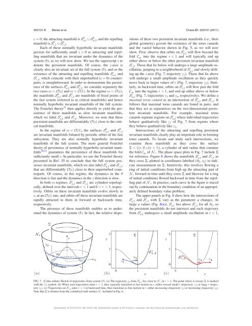
r;2 . Those that lie below will undergo a large amplitude oscillation,
jumping to a neighborhood of S e
a;1 and slowly drifting
up the z-axis (Fig. 7, trajectory c1). Those that lie above
will undergo a small amplitude oscillation as they quickly
move back to larger values of r (Fig. 7, trajectory c2). Similarly,
in backward time, orbits on S e
r;2 will flow past the fold
C into the regime r > 1, and end up either above or below
SN
S e
a;2 (Fig. 7, trajectories c3 and c4, respectively). We define a
maximal torus canard as an intersection of S e
a;2 and Ser;2
. It
follows that maximal torus canards are found in pairs, and
that they act as separatrices on the two-dimensional persistent
invariant manifolds. For example, maximal torus
canards separate regions on S e
a;2 where individual trajectories
behave qualitatively like c1 of Fig. 7 from regions where
they behave qualitatively like c2. Intersections of the attracting and repelling persistent
invariant manifolds clearly play an important role in forming
torus canards. To locate and study such intersections, we
examine these manifolds as they cross the surface
R ¼ fðr; h; zÞjr ¼ 1g, a cylinder of unit radius that contains
the fold C of N SN r. The phase space plots in Fig. 7 include R
for reference. Figure 8 shows the manifolds S e
a;2 and Ser;2
as
they cross R, plotted in coordinates labelled ðhR; zRÞ to indicate
measurement on R. Intuitively, this involves flowing a
ring of initial conditions from high up the attracting part of
N r forward in time until they cross R and likewise for a ring
of initial conditions flowed backward in time from the repelling
part of N r. In practice, each curve in the figure is traced
out by continuation in the boundary condition of an appropriately
defined boundary value problem.
The upper panels in Fig. 8 show how the intersections of
S e
a;2 and Ser;2
with R vary as the parameter a changes. At
large a values (Fig. 8(a)), S e
a;2 lies above Ser;2
for all hR, so
the persistent manifolds do not intersect and each trajectory
undergoes a small amplitude oscillation in r < 1,
from S e
a;2
FIG. 7. (Color online) Sketch of trajectories from system (5). (a) The trajectory c0 from S e
a;2 lies close to N r in r > 1. The point where it crosses R is marked
with the * symbol. (b) When such trajectories enter r < 1, they typically transition to fast motion in r, either toward small r (trajectory c1) or large r (trajectory
c2). (c) Trajectories on S e
r;2 enter r > 1 in backward time, then transition to fast motion in r, either decreasing (trajectory c3) or increasing (trajectory c4). Note that R is distinct from the cylindrical null-surface N z included in Fig. 6.
Downloaded 18 Feb 2012 to 168.122.67.168. Redistribution subject to AIP license or copyright; see http://chaos.aip.org/about/rights_and_permissions