An elementary model of torus canards - Mathematics & Statistics ...

An elementary model of torus canards 

G. Nicholas Benes, Anna M. Barry, Tasso J. Kaper, Mark A. Kramer, and John Burke a) 

Department of Mathematics and Statistics, Center for BioDynamics, Boston University, Boston, 

Massachusetts 02215, USA 

(Received 11 September 2010; accepted 29 April 2011; published online 27 June 2011) 

We study the recently observed phenomena of torus canards. These are a higher-dimensional 

generalization of the classical canard orbits familiar from planar systems and arise in fast-slow 

systems of ordinary differential equations in which the fast subsystem contains a saddle-node 

bifurcation of limit cycles. Torus canards are trajectories that pass near the saddle-node and 

subsequently spend long times near a repelling branch of slowly varying limit cycles. In this article, 

we carry out a study of torus canards in an elementary third-order system that consists of a rotated 

planar system of van der Pol type in which the rotational symmetry is broken by including a phasedependent 

term in the slow component of the vector field. In the regime of fast rotation, the torus 

canards behave much like their planar counterparts. In the regime of slow rotation, the phase 

dependence creates rich torus canard dynamics and dynamics of mixed mode type. The results of 

this elementary model provide insight into the torus canards observed in a higher-dimensional 

neuroscience model. VC 2011 American Institute of Physics. [doi:10.1063/1.3592798] 

Rhythms, and the transitions between different types of 

rhythms, are central objects of study in biology, chemistry, 

and neuroscience. Often these systems exhibit multiple 

time scales, resulting in so-called fast-slow systems. 

Rhythms in fast-slow systems typically consist either of 

alternating fast and slow segments or of fast oscillations 

whose amplitudes are modulated on longer time scales. 

In this article, we study the latter, specifically slow amplitude 

modulation of rapid oscillations in fast-slow systems 

which possess a family of attracting limit cycles and a 

family of repelling limit cycles. Normally, the attracting 

limit cycles are of primary importance, since they are the 

attractors for these systems. However, the repelling limit 

cycles also play crucial roles, in that they serve as boundaries 

between the basins of attraction of different attractors. 

Also, repelling limit cycles turn out to be crucial to 

the recently discovered phenomenon of torus canards. 

Torus canards spend long times near slowly varying families 

of attracting limit cycles and then near slowly varying 

families of repelling limit cycles, in alternation. They 

are the natural analog to the classical canards, which 

arise in the van der Pol equation and other planar, bistable 

models. The key ingredient for torus canards to occur 

is that the families of attracting and repelling limit cycles 

meet in a fold curve, also referred to as a saddle-node 

bifurcation of limit cycles. Torus canards have been 

observed in a mathematical model of action potential 

generation in Purkinje cells. Stable torus canard solutions 

exist for open sets of parameter values, correspond 

to amplitude-modulated spiking of the neural dynamics, 

and arise exactly in the transition region between rapid 

spiking and bursting in this model. Torus canards may 

appear in other bistable systems relevant to science and 

a) Author to whom correspondence should be addressed. Electronic mail: 

jb@math.bu.edu. 

CHAOS 21, 023131 (2011) 

engineering, such as in nonlinear optics, and may further 

understanding of mixed-mode oscillations (MMO) and 

the dynamics in the transition region between different 

types of oscillations. 

I. INTRODUCTION 

Canards are ubiquitous in systems exhibiting multiple 

time scales, see Refs. 2, 3, 6, 8, 14, 17–19, 27, 36–38, 43, 44, 

and 53 for some of the references. They were originally discovered 

3,14 in the van der Pol equation and arise generically 

when systems undergo Hopf bifurcations from spiral fixed 

points to full-blown periodic orbits of relaxation oscillation 

type. These canard solutions are periodic orbits that exist in 

narrow intervals of parameter values near the Hopf bifurcation 

point, and, most interestingly, these orbits spend long 

times near repelling slow manifolds. 2,13,18,37 Other planar 

systems possessing canards include the FitzHugh-Nagumo 

equation, 29 the Bonhoffer-van der Pol equation, 5 and the Kaldor 

equation. 25 

Canards also play central roles in systems exhibiting 

mixed-mode oscillations, see Refs. 7, 8, 12, 19, 26, 27, 44, 

and 53, as well as articles in the focus issue of Chaos. 7 Primary 

and secondary canards in these systems are the boundaries 

demarcating the regimes corresponding to periodic orbits 

with different numbers of small-amplitude oscillations (SAO) 

and large-amplitude oscillations (LAO). For example, these 

equations possess periodic orbits with a certain number of 

SAO followed by one LAO, as well as periodic orbits with 

the same number of SAO followed by two LAO, and the 

boundary between these two parameter regimes is given by a 

family of canards. Moreover, it is worth noting that these 

canards must exist in order for the property of continuous 

1054-1500/2011/21(2)/023131/17/$30.00 21, 023131-1 

VC 2011 American Institute of Physics 

Downloaded 18 Feb 2012 to 168.122.67.168. Redistribution subject to AIP license or copyright; see http://chaos.aip.org/about/rights_and_permissions

023131-2 Benes et al. Chaos 21, 023131 (2011) 

dependence of solutions on parameters to be preserved, just 

as for the van der Pol equation. 3,14 

In essentially all planar systems in which canards are 

known to occur, the critical underlying structure is that of a 

curve of attracting fixed points in the fast subsystem which 

merges with a curve of repelling fixed points at a fold (a.k.a., 

saddle-node) bifurcation. Indeed, in the van der Pol and other 

bistable planar systems, the cubic-like fast null-clines are the 

curves of fixed points, with the outer branches being attracting 

and the middle one repelling. Canard solutions spend 

long times near the middle, repelling branch. In systems with 

two slow variables and one fast variable, there are surfaces of 

attracting fixed points that merge with surfaces of repelling 

fixed points in curves of fold points, such as arise in the systems 

with MMO. There can also be MMO in systems with 

one slow and two fast variables, see for example Ref. 27. 

In this article, we examine the geometrically more complex 

situation in which families of attracting and repelling 

limit cycles (rather than fixed points) merge in a fold of limit 

cycles. The canards that arise are torus canards. They spend 

long times near the families of both attracting and repelling 

limit cycles, and they possess two frequencies, one intrinsic 

to the limit cycles and the other intrinsic to the alternation of 

fast jumps and slow segments. 

Torus canards were recently identified in a biophysical 

model of the Purkinje cell, 36 which is a neuron found in the 

cerebellar cortex (other mathematical models exploring bifurcations 

in Purkinje cells include Refs. 22–24). This model, 

briefly reviewed in Sec. II, consists of five first-order ordinary 

differential equations (ODEs), for the voltage, three gating 

variable corresponding to fast ionic currents, and one gating 

variable corresponding to a slow ionic current. Torus canards 

manifest themselves as quasi-periodic oscillations and appear 

during the transition between the bursting and rapid spiking 

states of the Purkinje cell model. As discussed in Ref. 36, the 

presence of torus canards may suggest some biophysical 

mechanisms that govern the activity in more realistic models 

of Purkinje cells. In many neural models, complicated dynamics 

often appears in the transition interval between bursting 

and rapid spiking states, so a better understanding of 

torus canards may contribute to the general study of these 

transitions, as well. 

Our main contribution here is to analyze an example of 

torus canards in a more rudimentary setting, which allows 

us to develop new insights into the results of Ref. 36. We 

begin with an extremely simple third-order system of ODEs 

which is obtained by rotating a planar system of van der Pol 

type about the axis corresponding to the slow recovery variable. 

As expected, we find that these torus canards are simply 

rotations of the classical canards of the planar problem, 

so all the known results from the planar case carry over in a 

straightforward way. In particular, the family of canards 

exists here in an exponentially narrow interval of the bifurcation 

parameter. 

We now introduce the main model of interest in this article. 

It is obtained by breaking the rotational symmetry in a 

rotated planar system of van der Pol type, 

_r ¼ rðz f ðrÞÞ ; (1a) 

_z ¼ e a 

_h ¼ x ; (1b) 

ffiffiffiffiffiffiffiffiffiffiffiffiffiffiffiffiffiffiffiffiffiffiffiffiffiffiffiffiffiffiffiffiffiffiffiffiffi 

r2 2rb cos h þ b2 p 

; (1c) 

where f(r) ¼ 2r 3 –3r 2 þ 1, and e, x, a, b are parameters with 

0 < e 1. The symmetry breaking term in system (1) is 

specifically chosen to shift the null-surface of the slow z variable 

by a distance b in the Cartesian x-direction. The voltage-like 

variable in this system is the cartesian y coordinate, 

so r measures the amplitude or envelope of the underlying 

oscillation. In what follows, we show that the symmetry 

breaking term is the key feature that gives rise to nontrivial 

torus canards and MMO. In particular, we will show that the 

parameter regime in which torus canards exist in system (1) 

is measurably larger than in the rotationally symmetric case, 

and the alternations between LAO and SAO are rich, since 

these transitions now also depend on orbital phase. 

We will show that the dynamics of torus canards in the 

third-order system (1) depends critically on x, the rate of 

rotation. For fast rotations, the canards exist only in narrow 

intervals of parameter values, similar to the rotationally symmetric 

case. In contrast, it is in the regimes of intermediate 

and slow rotations that we find a wide range of dynamics of 

torus canards and MMO. We present a combination of analytical 

and numerical results to explore the behavior of torus 

canards in these different regimes. 

The results we obtain for system (1) also yield new 

insight into the dynamics of the torus canards observed in the 

Purkinje cell model of Ref. 36. Specifically, we will show 

that in system (1) torus canards and MMO become more robust 

when the rotation rate x decreases, and we find a similar 

result when we decrease the spike frequency for the fifthorder 

Purkinje cell model. We refer the reader to Refs. 1, 11, 

32, 33, 40, 46, 50, and 52 for general treatments of bursting 

in mathematical models in neuroscience, as well as to Refs. 

47 and 48 for canards in maps, another class of problems for 

which the analysis here may have further implications. 

It is possible to convert system (1) into a two-dimensional 

forced oscillator by integrating the _ h component. The 

results presented here for system (1) complement those presented 

earlier in Refs. 4 and 27, where a different class of 

forced van der Pol oscillators is studied. In those works, the 

forcing replaces the parameter a from the planar system with 

an effective value of a sinðxtÞ, so the amplitude of the forcing 

is large and the slow null-cline moves back-and-forth between 

the two outer (attracting) branches of the fast null-cline each 

period. The analogous forcing term in the system studied here 

is, for small b, given by a þ b cosðxtÞ, so the slow null-cline 

remains in the neighborhood of a fold of the fast null-cline. 

This article is organized as follows. In Sec. II, we review 

the torus canard phenomena as observed in Ref. 36. In 

Sec. III, we briefly present results for the simple rotated planar 

system. In Sec. IV, we present the main third-order 

model studied in this article and describe the torus canards 

that it possesses. The analyses of the regimes of fast rotation 

and slow rotation are given in Secs. V and VI, respectively. 

In Sec. VII, we show that our conclusions carry over to a 

large class of systems with general phase-dependent 


023131-3 An elementary model of torus canards Chaos 21, 023131 (2011) 

symmetry breaking terms. Finally, in Secs. VIII and IX, we 

present some of the implications of our main results for the 

Purkinje model, and we discuss some other conclusions and 

open questions. 

II. MOTIVATION: PURKINJE MODEL 

In this section, we briefly describe the torus canard phenomenon 

as observed in an elementary biophysical model of 

a Purkinje cell. 36 This single-compartment model consists of 

five ODEs that describe the dynamics of the membrane potential 

(V) and four ionic gating variables (m CaH , h NaF , m KDR , and 

m KM ) 

C _ 

V ¼ J g L ðV V L Þ g CaH m 2 

CaH ðV V CaH Þ 

g NaF m 3 

NaF;1 h NaF ðV V NaF Þ 

g m KDR 4 

KDRðV VKDRÞ gKMm4 KMðV V Þ; (2a) 

KM 

_m CaH ¼ a CaH ð1 m CaH Þ b CaH m CaH ; (2b) 

_h NaF ¼ a NaF ð1 h NaF Þ b NaF h NaF ; (2c) 

_m KDR ¼ a KDR ð1 m KDR Þ b KDR m KDR ; (2d) 

_m KM ¼ a KM ð1 m KM Þ b KM m KM : (2e) 

The parameter J represents an externally applied current, 

with decreased values corresponding to excitation and 

increased values to inhibition. The forward and backward 

rate functions (aX and b X for X ¼ CaH, NaF, KDR, KM) and 

fixed parameters in Eq. (2a) are defined in Appendix. The 

gating variable m KM for the muscarinic receptor suppressed 

potassium current (a.k.a., M-current) evolves on a much 

slower time scale than the other variables. As such, the dynamics 

in this five-dimensional model can be understood in 

part by studying the four-dimensional fast subsystem, which 

is defined by setting _m KM ¼ 0 and treating m KM as a bifurcation 

parameter in the remaining equations. 

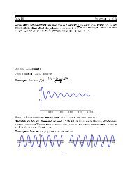
Figure 1 shows the behavior of the full Purkinje model 

at three different values of J, corresponding to examples of 

rapid spiking, amplitude modulated spiking, and bursting. In 

each case, the figure includes a time series of the voltage 

from the full model and the bifurcation diagram for the fast 

subsystem. The former are computed by numerically integrating 

system (2) with an arbitrary initial condition and disregarding 

the transient. The latter are traced out by 

continuation methods using AUTO (Ref. 15). Each bifurcation 

diagram includes a branch of attracting fixed points 

which merges with a branch of repelling fixed points in a 

FIG. 1. (Color online) Behavior of the Purkinje cell model (2) at three different values of J: (a) rapid spiking, at J ¼ 34 nA; (b) amplitude modulated spiking, 

at J ¼ 32.94 nA; (c) bursting, at J 32:93 nA. In each case, the left panel shows the time-series of the voltage, and the right panel shows the bifurcation 

diagram of the corresponding fast subsystem with the trajectory from the full system superimposed. In the fast subsystem, the branches of attracting (solid 

line) and repelling (dotted line) fixed points merge in a fold ( ). The branches of attracting (solid line) and repelling (dashed line) limit cycles merge in a fold 

of limit cycles ( ). The branch of repelling limit cycles terminates on the branch of repelling fixed points in a homoclinic bifurcation (D). Two curves are plotted 

for each branch of limit cycles, indicating the maximum and minimum values of V over the period. 



fold of fixed points and a branch of attracting limit cycles 

which merges with a branch of repelling limit cycles in a 

fold of limit cycles. Topologically, the branches of limit 

cycles are cylinders but for simplicity we plot only the maximum 

and minimum values of V over the period. In each 

case, the solution of the full system is also shown superimposed 

on the bifurcation diagram of the fast subsystem, and 

it is this composition which provides the most insight into 

the dynamics in each regime. 

For J sufficiently small (excitatory), trajectories of the 

full system approach a stable limit cycle which corresponds to 

rapid spiking of the neuron (Fig. 1(a)). The slow variable m KM 

is nearly constant in this state, and the trajectory of the full 

system closely resembles an orbit from the branch of stable 

limit cycles of the fast subsystem. At a larger value of J, the 

system undergoes amplitude modulated spiking (Fig. 1(b)). In 

this case, the trajectory closely follows the branch of attracting 

limit cycles of the fast subsystem as m KM slowly increases 

to the fold point, then follows the branch of repelling limit 

cycles as m KM slowly decreases beyond the fold. Eventually, 

the trajectory leaves this repelling branch and quickly transitions 

back to the attracting branch of limit cycles, restarting 

the sequence. Further increase in J introduces an interval of 

quiescence in the full dynamics (Fig. 1(c)). This occurs when 

the trajectory leaves the fast subsystem’s branch of repelling 

limit cycles and approaches the branch of attracting fixed 

points (rather than the branch of attracting limit cycles). The 

quiescence ends when the trajectory reaches the fold of fixed 

points and quickly transitions back to the branch of attracting 

limit cycles. This pattern of quiescence and rapid spiking 

repeats to generate bursting activity in the full system. Finally, 

we note that for J sufficiently large (inhibitory) the Purkinje 

cell model exhibits unmodulated quiescence corresponding to 

a stable fixed point of the system (not shown). 

The transition from stable rapid spiking to stable amplitude 

modulated spiking occurs via a supercritical torus bifurcation 

in the full system, as shown in Ref. 36. The growth of 

amplitude modulated spiking and the eventual transition to 

bursting in this model involves torus canards. These arise at 

precisely those J values for which certain invariant manifolds 

intersect. In particular, Fenichel theory yields that outside 

a neighborhood of the fold of limit cycles, the cylinders 

of attracting and repelling limit cycles in the fast subsystem 

persist as attracting and repelling invariant manifolds when 

m KM evolves slowly, say _m KM ¼OðÞ. These persistent invariant 

manifolds are smooth and located a small Oð Þ distance 

away from the cylinders of the fast subsystem. The persistent 

invariant manifolds can be extended into the neighborhood 

of the fold of limit cycles by flowing orbits on them forward 

and backward in time. A torus canard is a trajectory that 

spends long time near the attracting manifold, passes through 

the fold, then spend long time near the repelling manifold; 

thus, torus canards occur whenever the attracting and repelling 

manifolds intersect. 

III. THE ROTATED PLANAR SYSTEM 

In this section, we introduce one of the simplest thirdorder 

systems that possesses torus canards, namely we con- 

sider a planar system of van der Pol type, rotated about the 

axis corresponding to the slow recovery variable 

_r ¼ rz ð f ðrÞÞ; 

(3a) 

_h ¼ x ; (3b) 

_z ¼ eðarÞ; (3c) 

where f(r) ¼ 2r 3 –3r 2 þ 1 and e, a, x are parameters with 

0 < e 1. The parameter a is the control parameter that is 

important for canard behavior. Away from r ¼ 0 and for any 

fixed choice of h, the resulting planar cross section of the full 

system (3) has null-clines which resemble those of the classical 

van der Pol oscillator. Furthermore, the h-dynamics 

decouples from the r – z system, so in the full system one 

sees the usual dynamics of a van der Pol oscillator except 

that the fast variable r is interpreted as the amplitude or envelope 

of an underlying oscillation with frequency x. The 

torus canards in Eq. (3) are therefore a trivial extension of 

planar canards to a three dimensional system, and the important 

properties of these torus canards (e.g., range of existence) 

are identical to those in the planar case, as described 

below. 

The phase space of the r – z system (in the relevant domain 

r > 0) is sketched in Fig. 2. The z-null-cline consists of 

the vertical line r ¼ a. The r-null-cline consists of two 

branches—the vertical line r ¼ 0 and the curve z ¼ f(r), 

which has a local maximum at (r, z) ¼ (0, 1) and a local minimum 

at (r, z) ¼ (1, 0). In general, the flow circulates clockwise 

around the fixed point at the intersection of the nullclines, 

at (r, z) ¼ (a, f(a)). 

Within the fast subsystem z is a fixed parameter, so the 

r-dynamics exhibits a subcritical bifurcation at (r, z) ¼ (0, 1), 

with the nontrivial branch restabilized by the cubic term at 

large amplitude. Thus, trajectories flow away from the 

FIG. 2. (Color online) Sketch of the phase space of the r – z system from 

Eq. (3), including the null-clines for a ¼ 1.1. The z-null-cline is plotted as a 

dot-dashed line. The r-null-cline is plotted as a solid (dashed) line where it 

corresponds to a stable (unstable) fixed point of the fast subsystem. The 

null-clines intersect at the fixed point (r, z) ¼ (a, f(a)), marked with the 

symbol. The two-dimensional flow across the null-clines is indicated by single 

arrows, and the one-dimensional flow in the fast subsystem is indicated 

by double arrows. Only r > 0 is considered. 



repelling branches of the r-null-cline (r ¼ 0 in z > 1 and the 

segment of the f(r) curve in 0 < r < 1), rapidly converging 

to the attracting branches (r ¼ 0 in z < 1 and the outer segments 

of the f(r) curve). 

The fixed point at (r, z) ¼ (a, f(a)) of the r – z system 

undergoes a Hopf bifurcation at a ¼ 1. This may be seen 

from linear stability analysis. Let R and Z be defined by 

(r, z) ¼ (a, f(a)) þ (R, Z). The linearization is 

_R 

_ 

Z 

¼L R 

Z 

; where L 

6a 2 ða 1Þ a 

e 0 

; (4) 

so that TrL ¼ 6a 2 ða 1Þ and DetL ¼ea, and the eigenvalues 

r which determine the linear growth rate of perturbations 

from the fixed point satisfy 0 ¼ r 2 r TrLþDetL. 

When a is sufficiently greater than one, both eigenvalues are 

real (ðTrLÞ 2 > 4DetL) and negative (TrL < 0). At ðTrLÞ 2 ¼ 

4DetL, corresponding to a 1 þ e 1=2 =3, the eigenvalues 

become complex with Rer < 0 so the fixed point remains 

stable. At a ¼ 1, we have TrL ¼0 and r ¼ 6ie 1=2 as the 

eigenvalues cross the Imr axis. In a < 1, the eigenvalues 

have Rer > 0, and the fixed point is unstable. Thus, the fixed 

point undergoes a Hopf bifurcation at a ¼ 1. Note that this 

corresponds in the phase space diagram to the instant when 

the z-null-cline crosses the local minimum of the r-null-cline 

at (r, z) ¼ (1, 0). Using standard techniques of normal-form 

analysis, one can show that this Hopf bifurcation is always 

supercritical, so stability is transferred to the branch of small 

amplitude periodic orbits in a < 1. 

To illustrate the dynamics of this model, various orbits 

from the branch of limit cycles are shown in Fig. 3, plotted 

in the r – z phase space. The amplitude of the limit cycles is 

small near onset and grows as a decreases. Eventually, the 

periodic orbit undergoes a rapid jump in amplitude corresponding 

to the canard explosion. The bifurcation diagram in 

Fig. 4(a) summarizes the growth of the periodic orbit. A simple 

geometric argument explains these results. First, note 

that Fig. 3 also includes the r-null-cline, which consists of 

the branches of attracting and repelling fixed points of the 

fast subsystem. Fenichel theory yields that outside a neighborhood 

of the fold at (r, z) ¼ (1, 0), these critical manifolds 

persist as attracting and repelling slow manifolds when e is 

small but nonzero. These persistent slow manifolds are onedimensional, 

so each corresponds to a single trajectory that 

can easily be extended into the neighborhood of the fold by 

following the orbit forward or backward in time. Near the 

Hopf bifurcation, the attracting slow manifold spirals 

directly in to the small amplitude periodic orbit, so the 

attracting slow manifold must lie above the repelling slow 

manifold. At smaller values of a, where the stable periodic 

orbit is instead a large amplitude relaxation oscillation, the 

attracting slow manifold must lie below the repelling slow 

manifold. Continuity requires that these manifolds pass 

through each other as a decreases, and it is this crossing that 

creates the canard explosion. Canard orbits only occur in the 

narrow range of a values for which these manifolds are sufficiently 

close as to allow a single trajectory to spend considerable 

time in the neighborhood of both. The maximal 

canard occurs at the unique a value at which the attracting 

FIG. 3. (Color online) Collection of representative periodic orbits associated 

with the canard explosion at (a) e ¼ 0:1 and (b) e ¼ 0:02. In each panel, the 

orbits shown represent the limit cycles for a range of a values rather than 

solutions at a particular value of a. The canard explosion shown in (b) is already 

sufficiently abrupt that all the unlabeled orbits in this panel occur at 

nearly identical a values, a 0:9988723. 

and repelling slow manifolds intersect and can be identified 

in Fig. 4(b) as the limit cycle with the maximum period. 

Both the location in a and the abruptness of the explosion 

are functions of e: for smaller e, the canard explosion occurs 

closer to a ¼ 1 (i.e., closer to the Hopf point) and in a smaller 

range of values of a. Under an appropriate change of variables, 

the r – z system from Eq. (3) can be put into the canonical 

form given by Ref. 37, and the results from that paper 

predict the maximal canard occurs at a 1 e=18. For 

completeness, we note that some of the solutions also have 

long segments near the repelling branch of the z-axis, see, 

for example, the two outermost orbits in Fig. 3(b). Hence, 

they are also canards because they are near a repelling slow 

manifold for a long time, although we do not focus on this 

aspect of the solutions in this work. 

The behavior of torus canards in the full three-dimensional 

system (3) is now clear. In a > 1, the system contains 

a stable limit cycle with frequency x and radius r ¼ a. At 

a ¼ 1, the limit cycle becomes unstable in a supercritical torus 

bifurcation. The tori in a < 1 resemble donut-shaped 



FIG. 4. (Color online) (a) Bifurcation diagram of the r – z system from Eq. 

(3) for several values of e. The branch of fixed points undergoes a Hopf 

bifurcation at a ¼ 1; this branch is plotted as a solid (dotted) line where it is 

stable (unstable). Each branch of limit cycles (one per e value) is plotted as 

two curves, corresponding to the maximum and minimum values of r over 

the cycle. (b) The period of the orbits for each of the three values of e. The 

period at onset is T ¼ 2p= ffiffi e 

p and is indicated with the symbol. 

rotations of the periodic orbits from the planar system shown 

in Fig. 3. The first frequency identified with the tori is fixed at 

x, while the second frequency varies with a and is associated 

with motion in the r – z cross-section (Fig. 4(b)). The location 

in a and abruptness of the torus canard explosion are identical 

to the planar case for the same e. Near the torus bifurcation, 

the orbits around the tori are SAO which remain in the neighborhood 

of r ¼ 1. Beyond the torus canard explosion (i.e., 

smaller a), the orbits around the tori are LAO which include 

periods of quiescence as the trajectory passes near r ¼ 0. 

Therefore, small and large amplitude oscillations in system 

(3) occur in mutually exclusive ranges of the parameter 

a, and as a result this system does not include any MMO. 

For MMO to exist, one would need a trajectory to alternate 

between SAO and LAO at a fixed value of a. In what follows, 

we show that breaking the rotational symmetry of system 

(3) generates MMO by creating a region where SAO 

and LAO coexist, depending on the phase of the orbit. 

Remark: System (3) is similar to the equations used in 

Refs. 30 and 31 to model elliptic bursters—i.e., a two dimensional 

fast-slow system that exhibits canard behavior, trivially 

extended to three dimensions by rotation about a slow 

null-cline. The resulting dynamics of a single elliptic burster 

is consistent with the description presented here for the dynamics 

of system (3). Those works focus on the synchronization 

properties of networks of bursters, where the rotational 

symmetry of the individual burster is effectively broken by 

phase dependent coupling to the rest of the network. 

Remark: For orbits on the torus, there is the possibility 

of resonance between the two frequencies associated with 

the motion. In the regime of large x, these are higher order 

resonances—i.e., Oðe 1 Þ : 1—and do not have a noticeable 

effect on the dynamics. However, these resonances may play 

an important role in the regime of small x; see Ref. 39 for a 

discussion of this effect in the context of a mechanical selfoscillator. 

IV. THE MAIN THIRD-ORDER SYSTEM AND ITS 

TORUS CANARDS 

In this section, we introduce the main third-order system 

that we study and show the torus canards that it possesses. 

As stated in the Introduction, we obtain the main system (1) 

by adjusting the _z equation to shift the z-null-surface a distance 

b in the cartesian x-direction, thereby breaking the 

phase invariance of the rotated planar system (3). The equations 

are 

_z ¼ e a 


_h ¼ x ; (5b) 

ffiffiffiffiffiffiffiffiffiffiffiffiffiffiffiffiffiffiffiffiffiffiffiffiffiffiffiffiffiffiffiffiffiffiffiffiffi 

r2 2rb cos h þ b2 p 

; (5c) 

where b > 0 is the parameter that controls the strength of the 

symmetry breaking, and we recall that f(r) ¼ 2r 3 –3r 2 þ 1. In 

Cartesian coordinates, this system is 

_x ¼ xðz 

ffiffiffiffiffiffiffiffiffiffiffiffiffiffi 

f ð x2 þ y2 p 

ÞÞ xy ; (6a) 

_y ¼ yðz 

ffiffiffiffiffiffiffiffiffiffiffiffiffiffi 

f ð x2 þ y2 p 

ÞÞ þ xx ; 

ffiffiffiffiffiffiffiffiffiffiffiffiffiffiffiffiffiffiffiffiffiffiffiffiffiffi 

(6b) 

_z ¼ e a ðx bÞ 2 þ y2 q 

: (6c) 

The vector field is not analytic at fðx; y; zÞjx ¼ b; y ¼ 0g due 

to the branch point of the square root in the _z equation, but 

this does not affect the torus bifurcation or the creation of 

torus canards which are of interest here. Furthermore, while 

we focus on a general choice of f ðrÞ here, one can assume 

analyticity also at r ¼ 0 by choosing f ðrÞ to be a function of 

r 2 only. Generalizations of this system that include arbitrary 

symmetry breaking terms and do not suffer from this branch 

point are presented in Sec. VII. 

Notice that system (5) includes three time scales, 

because the OðxÞ dynamics of the h-variable is now coupled 

to the fast Oð1Þ and slow OðeÞ dynamics familiar from the 

planar case. In the analysis that follows, we focus on the two 

regimes where x is comparable to either the fast or the slow 

dynamics. In the former, x ¼Oð1Þ so system (5) includes 

one slow and two fast variables. In the latter, x ¼OðeÞ so 

system (5) includes two slow and one fast variables. We also 

present numerical results for intermediate values of x. 

We begin with a brief description of the wide range of 

dynamics exhibited by system (5), as shown in Fig. 5. At sufficiently 

large a > 1, the system exhibits stable, uniform amplitude 

spiking at frequency x. As a decreases, uniform 

amplitude spiking becomes unstable, and stability is transferred 

to SAO (Fig. 5(a), where the envelope r(t) remains 

close to r ¼ 1). At different values of a, the system exhibits 

LAO (Fig. 5(c), where r(t) spends some time in the 



FIG. 5. (Color online) (a–c) Behavior of system (5) at three different values 

of the parameter a: (a) SAO, at a ¼ 0.9945; (b) MMO, at a ¼ 0.99398; (c) 

LAO, at 0.9935. In each of these panels, the remaining parameters are fixed 

at b ¼ 0.01, e ¼ 0:1, x ¼ 0:9 and the plot includes both yðtÞ ¼rðtÞ sin hðtÞ 

and the envelope r(t). (d) MMO at a ¼ 0.99398, b ¼ 0.01, e ¼ 0:1, x ¼ 0:01, 

corresponding to slow rotation. For clarity, only r(t) is included in this 

frame. (e) Summary of the dynamics exhibited by system (5), shown in the 

ðx; aÞ parameter plane at b ¼ 0.01, e ¼ 0:1. The boundaries in (e) were computed 

using the continuation technique outlined in the Remark at the end of 

Sec. IV. 

neighborhood of r ¼ 0) and MMO (Fig. 5(b), where the trajectory 

alternates between large and small amplitude oscillations). 

As shown in Fig. 5(e), the MMO occur over a range 

of intermediate a values between the regions of SAO and 

LAO, and this range in a varies with x. The MMO are more 

robust for small x (i.e., the two slow and one fast regime) 

but persist for large x (i.e., the one slow two fast regime). In 

what follows, we show that torus canards are responsible for 

creating the MMO region. 

We now proceed with the analysis of system (5). It is 

useful to define two surfaces in the three dimensional phase 

space of this system, 

N r ¼ fðr; h; zÞjz ¼ f ðrÞg; 

N z ¼ ðx; y; zÞja 2 ¼ðx bÞ 2 þ y 2 

n o 

: 

(7) 

FIG. 6. (Color online) The null-surfaces N r and N z of system (5). The 

curve C SN traces out the local minimum of N r. The point P0 is a local maximum 

of N r. The curve at the intersection of these two null-surfaces 

(N r \ Nz) is shown for reference. The lower part of the figure shows a projection 

onto the (x, y) plane. The projection of C SN is a circle of unit radius, 

centered at the origin. The projection of N z is a circle of radius a, centered 

at (x, y) ¼ (b, 0). In this figure, a ¼ 1.3 and b ¼ 0.2. 

These are plotted in Fig. 6. The surface N z is the z-nullsurface 

of Eq. (5). It is a cylinder of radius a with axis 

fðx; y; zÞjx ¼ b; y ¼ 0g. Inside the cylinder, _z is positive, and 

outside it is negative. The surface N r is the main branch of 

the r-null-surface of Eq. (5)—above the surface _r is positive 

and below it is negative; the other branch of the r-null-surface 

is the z-axis. The curve C ¼ fðr; h; zÞjr ¼ 1; z ¼ 0g 

SN 

traces out the fold at the local minimum of N r, and the point 

P0 ¼ fðr; h; zÞjr ¼ 0; z ¼ 1g is a local maximum of this 

surface. 

The surface N r, excluding a small neighborhood of CSN and P0, is a normally hyperbolic invariant manifold of system 

(5) when e ¼ 0, as is N z with a neighborhood of P0 

excluded. In the remainder of this section, we briefly examine 

how these manifolds persist for 0 < e 1, using Fenichel 

theory, 21,34 following in particular the presentation of 

Ref. 35. We exclude small neighborhoods of the ring C and SN 

the point P0, where the manifolds are not normally hyperbolic. 

We label the different segments of these manifolds 

according to whether they are attracting or repelling in the 

fast subsystem, with the subscripts a and r denoting attracting 

and repelling, respectively. Let S 0 

a;1 denote the portion of 

the z-axis with z < 1, which is the attracting portion of this 

critical set, and include the superscript zero to denote e ¼ 0. 

Let S 0 

r;1 be the portion of the z-axis with z > 1, which is the 

repelling portion. Next, let S 0 

a;2 denote the attracting portion 

of the null-cline N r, i.e., that portion with r > 1, and, let 

be that portion with 0 < r < 1 which is repelling. So at 

Downloaded 18 Feb 2012 to 168.122.67.168. Redistribution subject to AIP license or copyright; see http://chaos.aip.org/about/rights_and_permissions 

S 0 

r;2


e ¼ 0, the attracting manifold is S 0 

a;1 [S0a;2 

, and the repelling 

manifold is S 0 

r;1 [S0r;2 

. 

Each of these normally hyperbolic invariant manifolds 

persists for sufficiently small e > 0 as attracting and repelling 

manifolds that are invariant under the dynamics of the 

system (5), as we will now show. We use the superscript e to 

denote the persistent manifolds. Of course, the z-axis is 

clearly also an invariant set of the full system (5), and so the 

existence of the attracting and repelling manifolds S e 

a;1 and 

S e 

r;1 , which coincide with their unperturbed (e ¼ 0) counterparts, 

is straightforward. In order to demonstrate the persistence 

of the surfaces S 0 

a;2 and S0r;2 

, we consider separately the 

two cases x ¼OðeÞand x ¼Oð1Þ. In the regime x ¼OðeÞ, 

the manifolds S 0 

a;2 and S0r;2 

are manifolds of fixed points of 

the fast system (referred to as critical manifolds) and hence 

normally hyperbolic invariant manifolds of the full system. 

The Fenichel theory 21 then applies directly to yield the persistence 

of these manifolds as slow invariant manifolds, 

which we label S e 

a;2 and Ser;2 

. Moreover, we note that these 

persistent manifolds are differentiably OðeÞ close to the critical 

manifolds. 

In the regime of x ¼Oð1Þ, the surfaces S 0 

a;2 and S0r;2 

are invariant manifolds foliated by periodic orbits of the fast 

subsystem. They are also normally hyperbolic invariant 

manifolds of the full system. The more general Fenichel 

theory of persistence of normally hyperbolic invariant manifolds 

20,21 guarantees the persistence of these manifolds for 

sufficiently small e. In particular, we use the Fenichel theory 

presented in Ref. 35 to conclude that the full system possesses 

invariant manifolds, which we also label S e 

a;2 and Ser;2 

, 

that are differentiably OðeÞ close to their unperturbed counterparts. 

Of course, in this regime, the dynamics in the h 

direction is fast and the dynamics in the z direction is slow. 

In both x regimes, S e 

sitions of these two persistent invariant manifolds (i.e., their 

global geometry) govern the existence of the torus canards 

and the varied behavior shown in Fig. 5, as we will now 

show. First, observe that orbits on S 

a;2 and Ser;2 

are cylinders topologically, 

defined over the intervals r > 1 and 0 < r < 1, respectively. 

Orbits on these invariant manifolds evolve slowly in 

z, at an OðeÞ rate, and orbits off these invariant manifolds are 

rapidly attracted to them in forward or backwards time, 

respectively. 

The presence of these manifolds enables us to understand 

the dynamics of system (5). In fact, the relative dispo- 

e 

a;2 will flow beyond the 

fold C into the regime r < 1 and will typically end up 

SN 

either above or below the other persistent invariant manifold 

S e 

r;2 . Those that lie below will undergo a large amplitude oscillation, 

jumping to a neighborhood of S e 

a;1 and slowly drifting 

up the z-axis (Fig. 7, trajectory c1). Those that lie above 

will undergo a small amplitude oscillation as they quickly 

move back to larger values of r (Fig. 7, trajectory c2). Similarly, 

in backward time, orbits on S e 

r;2 will flow past the fold 

C into the regime r > 1, and end up either above or below 

SN 

S e 

a;2 (Fig. 7, trajectories c3 and c4, respectively). We define a 

maximal torus canard as an intersection of S e 

a;2 and Ser;2 

. It 

follows that maximal torus canards are found in pairs, and 

that they act as separatrices on the two-dimensional persistent 

invariant manifolds. For example, maximal torus 

canards separate regions on S e 

a;2 where individual trajectories 

behave qualitatively like c1 of Fig. 7 from regions where 

they behave qualitatively like c2. Intersections of the attracting and repelling persistent 

invariant manifolds clearly play an important role in forming 

torus canards. To locate and study such intersections, we 

examine these manifolds as they cross the surface 

R ¼ fðr; h; zÞjr ¼ 1g, a cylinder of unit radius that contains 

the fold C of N SN r. The phase space plots in Fig. 7 include R 

for reference. Figure 8 shows the manifolds S e 

a;2 and Ser;2 

as 

they cross R, plotted in coordinates labelled ðhR; zRÞ to indicate 

measurement on R. Intuitively, this involves flowing a 

ring of initial conditions from high up the attracting part of 

N r forward in time until they cross R and likewise for a ring 

of initial conditions flowed backward in time from the repelling 

part of N r. In practice, each curve in the figure is traced 

out by continuation in the boundary condition of an appropriately 

defined boundary value problem. 

The upper panels in Fig. 8 show how the intersections of 

S e 

a;2 and Ser;2 

with R vary as the parameter a changes. At 

large a values (Fig. 8(a)), S e 

a;2 lies above Ser;2 

for all hR, so 

the persistent manifolds do not intersect and each trajectory 

undergoes a small amplitude oscillation in r < 1, 

from S e 

a;2 

FIG. 7. (Color online) Sketch of trajectories from system (5). (a) The trajectory c0 from S e 

a;2 lies close to N r in r > 1. The point where it crosses R is marked 

with the * symbol. (b) When such trajectories enter r < 1, they typically transition to fast motion in r, either toward small r (trajectory c1) or large r (trajectory 

c2). (c) Trajectories on S e 

r;2 enter r > 1 in backward time, then transition to fast motion in r, either decreasing (trajectory c3) or increasing (trajectory c4). Note that R is distinct from the cylindrical null-surface N z included in Fig. 6. 



FIG. 8. (Color online) Plots of the manifolds S e 

a;2 and Ser;2 

as they cross the surface R, plotted in coordinates ðhR; zRÞ measured on R. The upper panels show 

the manifolds move through each other as a varies. (a) At a ¼ 1.00448, S e 

a;2 lies above Ser;2 

; (b) at a ¼ 0.99398, they intersect; (c) at a ¼ 0.98348, Sea;2 

lies 

below S e 

r;2 . Other parameters in (a–c): x ¼ 0:01, b ¼ 0.01, e ¼ 0:1. The lower panels show different regimes for the rotation rate: (d) fast, at x ¼ 0:9; (e) intermediate, 

at x ¼ 0:3; and (f) slow, at x ¼ 0:01. Other parameters in (d–f): a ¼ 0.99398, b ¼ 0.01, e ¼ 0:1. Intersections are indicated in each panel with the 

symbol. 

similar to c2 from Fig. 7. Decreasing the parameter a causes 

S e 

a;2 to move down and Ser;2 

to move up in zR, so at smaller a 

values (Fig. 8(c)), S e 

a;2 lies below Ser;2 

for all hR. In this case, 

each trajectory from S e 

a;2 undergoes a large amplitude oscillation 

in r < 1, similar to c1 from Fig. 7. At the intermediate 

value of a shown in Fig. 8(b) the manifolds intersect, so both 

large and small amplitude orbits are possible, depending on 

the initial condition. The lower panels in Fig. 8 show how 

the manifolds deform as x varies. At the particular a value 

used in these panels, the intersection of S e 

a;2 and Ser;2 

persists 

from small x (Fig. 8(f)) well into the regime of large x 

(Fig. 8(d)). As x increases, the hZ variation of the two manifolds 

becomes nearly identical and so the intersection 

becomes less robust to changes in the parameter a (which 

shift S e 

r;2 and Ser;2 

in opposite directions in zR). 

The persistence of the intersections of S e 

a;2 and Ser;2 

is in 

part a consequence of simple geometry. In the two-dimensional 

planar system described in Sec. III, the attracting and 

repelling slow manifolds were each one-dimensional invariant 

sets, so their intersection occurred at a unique value of the parameter 

a. In the three-dimensional system considered here, 

S e 

a;2 and Ser;2 

are each two-dimensional invariant surfaces. 

The one-dimensional intersections of such surfaces are structurally 

stable and therefore persist over a range of a values. 

The maximal torus canards lie along the intersections of 

S e 

a;2 and Ser;2 

. Torus canards occur near these intersections 

where the separation between the manifolds is necessarily 

small. Restricting our attention to trajectories on S e 

Fig. 8(b)), this strip of torus canards is narrow, including 

only a small fraction of the trajectories on S 

a;2 , this 

means that there is a strip of torus canard trajectories surrounding 

each maximal torus canard. When x is small (as in 

e 

a;2 . When x is 

larger (as in Fig. 8(d)), the strip of torus canards is broader 

and may grow to include the entire surface. 

The intersection of S e 

a;2 and Ser;2 

also implies the existence 

of MMO. A single MMO trajectory cycles through R 

many times, and for any nonzero x, the value of hR will in 

general change with each cycle. A detailed study of the 

sequence of hR values generated by the global return map 

R ! R is beyond the scope of this article. However, the 

global return does appear to mix the two ranges of hR that lie 

on either side of the maximal torus canards. We find numerically 

that the hR sequence almost always includes hR values 

where S e 

a;2 lie above Ser;2 

, as well as values where Se a;2 lies 

below S e 

r;2 . This explains why the range over which the persistent 

invariant manifolds S e 

a;2 and Ser;2 

intersect (and hence 

the range over which torus canards occur) matches exactly 

the range over which MMO are observed in Fig. 5(e). In the 

regime of small x, MMO consist of many SAO followed by 

many LAO due to the fact that the angle hR changes by a 

small amount each cycle (Fig. 5(d)). When x is larger, the 

MMO transitions more frequently between large and small 

amplitude oscillations (Fig. 5(b)). 

Note that the maximal torus canards are typically not 

global attractors of the dynamics of the full system (5) and 

need not appear in the MMO sequence. Nevertheless, the 

maximal torus canards allow S e 

a;2 to simultaneously include 

both SAO and LAO orbits, thereby playing a crucial role in 

guiding the long time dynamics of the system and creating 

MMO. 



FIG. 9. (Color online) Similar to Fig. 8, but at a larger value of b. Parameters: 

a ¼ 0.9955, b ¼ 0.1, e ¼ 0:1, x ¼ 0:9. 

Clearly, the magnitude of x is particularly important in 

determining how robust the torus canard phenomenon is to 

changes in parameters. We analyze the cases of large and 

small x in Secs. V and VI, confirming the numerical results 

about the persistent invariant manifolds, their intersections, 

and their separation. 

Remark: We have chosen to use the cylinder fr ¼ 1g as 

our cross-section R in the numerical simulations. As a result, 

there are threshold values of b (depending on a and x) such 

that the SAO and LAO in the numerical simulations will hit 

the cross-section only for values of b below the threshold. 

For example, in Fig. 9, we show the images of S e 

a;2 

and Se 

r;2 

on R for a value of b that is an order of magnitude larger 

than that used in Fig. 8 and that is just below the threshold. 

To observe the dynamics of the SAO, LAO, and MMO for 

larger values of b (with the other parameters fixed), one 

would need to use a different, more complicated cross-section 

that is tailored to the shape and amplitude of the symmetry-breaking 

term. In this sense, the threshold is artificial. 

We do not pursue other choices of cross-sections here. 

Remark: The above description focuses on locating the 

maximal torus canards by tracing out the manifolds S e 

a;2 

and S e 

r;2 , then searching for their intersections. The maximal 

torus canards can also be found directly as solutions to a 

boundary value problem, where the boundaries lie far up 

the attracting and repelling parts of N r. Numerical continuation 

of the maximal torus canards provides an efficient 

way to compute several important properties of these trajectories. 

For example, the tangencies between S e 

a;2 and Se 

r;2 

correspond to saddle-node bifurcations of the branch of 

maximal torus canards. The boundaries of the MMO region 

in Fig. 5(e) were computed directly in AUTO by continuation 

of these saddle-node bifurcations in two parameters, a 

and x. 

V. FAST ROTATION—AVERAGING FOR LARGE x 

In this section, we analyze the system (5) for large x 

using averaging. This corresponds to the regime in which 

system (5) includes one slow and two fast variables. We 

show that the system includes a periodic orbit which undergoes 

a torus bifurcation at 

a 1 þ b 2 =4 : (8) 

This torus bifurcation plays a similar role in the creation of 

torus canards as the Hopf bifurcation in the planar case. We 

employ the method of averaging 28,45 in the regime of large 

x to establish this basic result about the torus bifurcation. 

We limit the analysis here to the leading order averaging, 

and then, at the end of this section, comment on higher order 

effects. We present numerical evidence that the higher order 

effects are not crucial for the values of b considered here. 

We define h0 ¼ hð0Þ, so the _ h component of this system 

is trivially solved by hðtÞ ¼xt þ h0. The z-component of the 

vector field is periodic with period 2p=x. We use ~z to denote 

this variable in the averaged system, and let z ¼ ~z þ dfðr; ~z; tÞ 

with d ¼ OðebÞ. Then, 

and 

_z ¼ _~z þ d @f @f @f 

þ d _r þ d 

@t @r @~z _~z (9) 

1 

_~z ¼ 1 þ d @f 

@~z 

_z d @f 

_r 

@r 

@f 

d 

@t 

¼ 

@f 

1 þ d 

@~z 

e a 

ffiffiffiffiffiffiffiffiffiffiffiffiffiffiffiffiffiffiffiffiffiffiffiffiffiffiffiffiffiffiffiffiffiffiffiffiffiffiffiffiffiffiffiffiffiffiffiffiffiffiffiffiffi 

r2 2rb cosðxt þ h0Þþb2 p 

d @f 

_r 

@r 

@f 

d 

@t 

: 

1 

(10) 

We will choose the function f so that the oscillatory part of 

the square root is canceled from the above equation. With 

this goal in mind, it is natural to choose d ¼ eb instead of the 

weaker assumption that d ¼OðebÞ. Thus, 

1 

_~z ¼ e 1 þ eb @f 

@~z 


a r2 2rb cosðxt þ h0Þþb2 p 

b @f @f 

_r b 

@r @t 

: 

(11) 

Next, we show that _r ¼OðeÞalong the trajectories of interest. 

In particular, the initial conditions of these trajectories 

satisfy either rð0Þ > 1 or 0 < rð0Þ < 1. Provided the solution 

is outside a neighborhood of the fold C , it follows 

SN 

from Fenichel theory that the orbit will be exponentially 

attracted to S e 

a;2 in forward time or Ser;2 

in backward time, 

and in both cases _r ¼OðeÞto leading order. Therefore, for 

orbits for which r(t) stays outside of a small neighborhood of 

r ¼ 1, Eq. (11) simplifies to 

1 

_~z ¼ e 1 þ eb @f 

@~z 

ffiffiffiffiffiffiffiffiffiffiffiffiffiffiffiffiffiffiffiffiffiffiffiffiffiffiffiffiffiffiffiffiffiffiffiffiffiffiffiffiffiffiffiffiffiffiffiffiffiffiffiffi 

a r2 2rb cosðxt þ h0Þþb2 p 

b @f 

@t þOðe2 bÞ : 

(12) 

We separate the square root into a sum of its average and 

oscillatory parts using the identity 



ffiffiffiffiffiffiffiffiffiffiffiffiffiffiffiffiffiffiffiffiffiffiffiffiffiffiffiffiffiffiffiffiffiffiffiffiffiffiffiffiffiffiffiffiffiffiffiffiffiffiffi 

r2 2rb cosðxt þ h0Þþb2 p 

ðr bÞ 4br 

¼ E p; 

p ðr bÞ 2 

! 

ffiffiffiffiffiffiffiffiffiffiffiffiffiffiffiffiffiffiffiffiffiffiffiffiffiffiffiffiffiffiffiffiffiffiffiffiffiffiffiffiffiffiffiffiffiffiffiffiffiffiffi 

þ r2 2rb cosðxt þ h0Þþb2 p ðr bÞ 4br 

E p; 

p ðr bÞ 2 

" ! # 

; 

where Eð ; Þ is the incomplete elliptic integral of the second 

kind. 10 Clearly, if we choose f such that 

@f 

@t 

¼ 1 

b 


r2 2rb cosðxt þ h0Þþb2 hp 

ðr bÞ 

E 

p 

p; 

ðr 

4br 

bÞ 2 

!# 

; (13) 

then we see that f is independent of ~z so that @f=@~z ¼ 0 and 

Eq. (12) for ~z reduces to 

_~z ¼ e a 

ðr bÞ 

E 

p 

p; 

ðr 

4br 

bÞ 2 

" ! # 

þOðe 2 bÞ : (14) 

Equation (14) is the leading order averaged equation. For the 

values of b shown in Fig. 10, the leading order term dominates 

and the remainder is second order in e and also linearly 

proportional to b. 

The main result (8) about the torus bifurcation is now at 

hand. In particular, we expand the incomplete elliptic integral 

in powers of b and find 

_~z ¼ e a r 

b 2 

4r þOðeb3 ; e 2 bÞ : (15) 

Now, since the fold of N r is at r ¼ 1, it follows that the torus 

bifurcation should occur when a 1 þ b 2 =4, which establishes 

Eq. (8). This parabola is shown in Fig. 10 and fits well 

to the data points obtained from numerically computed torus 

bifurcations. 

FIG. 10. (Color online) Location of the torus bifurcation in system (5), plotted 

in the (a, b) parameter plane. Exact values for x ¼ 1 and e ¼ 0:1 are 

indicated with the symbol and were determined at several fixed b values 

by numerical continuation of periodic solutions in the parameter a. The 

approximation (8), derived from the leading order averaging, is plotted as a 

solid curve. 

For each value of b shown in Fig. 10, torus canards exist 

for a small interval of a values just below the torus bifurcation. 

While the first-order averaging is insufficiently sensitive 

to find these intervals analytically, they may be found 

(and we found them) numerically. They are narrow intervals 

and get narrower as x gets larger (data not shown). 

Remark: In using Eq. (15) in the limit that b ! 0, one 

has to exercise care with how small b is relative to e, as one 

of the remainder terms eventually becomes more important 

than the b 2 term in parentheses. We do not pursue this small 

correction for very small values of b here. 

Remark: It is important to note that the assumption 

made above that _r ¼OðeÞ only holds outside a small neighborhood 

of the fold C SN , because the Fenichel theory only 

applies outside this neighborhood. Nevertheless, the orbits 

we study here briefly pass through this neighborhood. Hence, 

to make the above averaging fully rigorous, one needs to use 

the theory of Ref. 42 to determine the size, which is Oðe p Þ 

for some 0 of _r in this brief interval. Also, it may be 

possible to get a much sharper bound on the closeness of the 

images on R in the regime of fast rotations (Fig. 8(d)) by 

using the ideas in Ref. 41. 

VI. SLOW ROTATION—BLOW-UP FOR SMALL x 

In this section, we use geometric desingularization 16 to 

understand the dynamics in the slow rotation regime. This 

corresponds to the regime in which system (5) includes two 

slow and one fast variables. The geometric desingularization 

method, which is also known as the blow-up method, enables 

one to naturally extend geometric singular perturbation 

theory 21,34 to fast-slow problems with relaxation oscillations 

to overcome the loss of hyperbolicity at fold points. 17,37,38 

As mentioned in Sec. IV, the MMO in system (5) become 

more robust when h is a slowly varying parameter—i.e., they 

occur over a wider range in the parameter a for each fixed 

value of b > 0. To better understand the dynamics in this regime, 

we assume x ¼ e ~x, where ~x is Oð1Þ with respect to e 

and adopt the blow-up method of Refs. 16, 17, and 49. In 

particular, we blow up the ring C SN along the fold of the rnull-surface 

N r. 

Since we are concerned with dynamics near r ¼ 1 (recall 

that C SN ¼ fðr; h; zÞjr ¼ 1; z ¼ 0g), we make a change of variables 

s ¼ r – 1 and introduce the new parameter k ¼ a 1. 

After expanding in powers of b, we find that system (5) 

becomes 

where 

_s ¼ zð1 þ sÞ 3s 2 

5s 3 

2s 4 ; (16a) 

_h ¼ e ~x ; (16b) 

_z ¼ eðgðs; h; k; bÞþhðs; h; bÞþOðb 3 ÞÞ ; (16c) 

_e ¼ 0 ; (16d) 

_k ¼ 0 ; (16e) 

_b ¼ 0 ; (16f) 

gðs; h; k; bÞ ¼ s þ k þ b cos h ; (17a) 



The blow-up is given by 

hðs; h; bÞ ¼ b 2 sin 2 h 

: (17b) 

2ð1 þ sÞ 

s ¼ qs ; z ¼ q 2 z ; e ¼ q 2 e ; k ¼ qk ; b ¼ qb ; (18) 

which defines a map 

U : S 5 ½0; dŠ S 1 ! R 3 R R R 

ðs; z; e; k; b; q; hÞ 7! ðr; h; z; e; k; bÞ : 

(19) 

The transformation Eq. (18) blows up the ring C SN into a cylinder, 

where the variable h is unaltered. We include both the 

coordinates and the parameters in the blow-up because we 

want to locate the maximal torus canards and also predict 

how they vary with the parameters. 

To analyze the blown-up dynamics, we will look at the 

charts K 1 and K 2 that correspond, respectively, to setting 

z ¼ 1 and e ¼ 1, 

K1 : s ¼ q 1s1 ; z ¼ q 2 1 ; e ¼ q2 1 e1 ; k ¼ q 1k1 ; b ¼ q 1b1 ; 

(20) 

K2 : s ¼ q 2s2 ; z ¼ q 2 2 z2 ; e ¼ q 2 2 ; k ¼ q 2k2 ; b ¼ q 2b2 : 

(21) 

The chart K1 is the entry and exit chart, which we will use to 

study how orbits enter and exit a neighborhood of C SN . The 

chart K 2 is the rescaling chart, which we will use to analyze 

the dynamics of orbits as they pass through the neighborhood 

of C SN . 

The change of coordinates j12 from K1 to K2 is given by 

s2 ¼ s1e 1=2 

1 ; z2 ¼ e 1 

1 ; k2 ¼ k1e 1=2 

1 ; b2 ¼ b1e 1=2 

1 ; 

(22) 

and j 1 

12 is given by 

s1 ¼ s2z 1=2 

2 ; e1 ¼ z 1 

2 ; k1 ¼ k2z 1=2 

A. Dynamics in the chart K 1 

2 ; b1 ¼ b2z 1=2 

2 : 

(23) 

This chart is used to analyze the dynamics around the 

entry into and exit from the fold region. After rescaling time 

by a factor of q 1, the equations of motion in this chart are 

_s1 ¼ 1 þ q 1s1 

3s 2 1 

1 

2 s1e1ðg þ q 1hÞ 5q 1s 3 1 2q 2 1 s4 1 ; 

(24a) 

_h ¼ q 1e1 ~x ; (24b) 

_e1 ¼ e 2 1ðg þ q1hÞþOðq 2 1Þ ; (24c) 

_q 1 ¼ 1 

2 q1e1ðg þ q1hÞþOðq 3 1Þ ; (24d) 

_k1 ¼ 1 

2 k1e1ðg þ q1hÞþOðq 2 1Þ ; (24e) 

_b1 ¼ 1 

2 b1eðg þ q1hÞþOðq 2 1Þ ; (24f) 

where g ¼ gðs1; h; k1; b1Þ and h ¼ hðq 1s1; h; b1Þ. In this 

chart, we have invariant hypersurfaces corresponding to each 

of e1 ¼ 0, q 1 ¼ 0, k1 ¼ 0, and b 1 ¼ 0; in the first two of these 

surfaces, any hypersurface h ¼ h0 2 S 1 is also invariant. The 

intersection of all these hypersurfaces is an invariant line, 

‘1 ¼ fðs1;h;e1;q 1;k1;b1Þjh ¼ h0;e1 ¼ 0;q1 ¼ 0;k1 ¼ 0;b1 ¼ 0g: 

This line has two equilibria, pa ¼ð1= ffiffi p 

3; 

h0; 0; 0; 0; 0Þ and 

pr ¼ð 1= ffiffiffi p 

3; 

h0; 0; 0; 0; 0Þ; theformerisattracting(onthe 

line) and the latter is repelling. The point pa has one stable 

eigenvector in the s direction and 5 zero eigenvalues in the 

directions of h, q, k, b, ands=12 ffiffiffi p 

3 þ e. Thepointprhas one unstable eigenvector in the s direction and 5 zero eigenvalues 

in the directions of h, q, k, b, and s=12 ffiffiffi p 

3 e. 

The normally hyperbolic invariant manifold S 0 

a;2 connects 

directly to pa. For small values of e > 0, orbits on the persistent 

invariant manifold S e 

a;2 enter the neighborhood of 

C near p SN a. Similarly, the normally hyperbolic invariant 

manifold S 0 

r;2 connects to pr, and for small e > 0, orbits on 

the persistent invariant manifold S e 

r;2 enter in backward 

time near pr. B. Dynamics in the chart K2 

This chart is used to analyze the flow from the point pa 

to the point pr—i.e., the flow through the blow-up region. 

After rescaling time by a factor of q 2, the dynamics here is 

_s2 ¼ z2ð1 þ q2s2Þ 3s 2 2 5q2s 3 2 2q 2 2s42 ; (25a) 

_h ¼ q 2 ~x ; (25b) 

_z2 ¼ g þ q 2h ; (25c) 

_q 2 ¼ 0 ; (25d) 

_k2 ¼ 0 ; (25e) 

_b2 ¼ 0 ; (25f) 

where g ¼ gðs2; h; k2; b2Þ and h ¼ hðq 2s2; h; b2Þ. In the 

invariant surface q 2 ¼ 0, we have 

_s2 ¼ z2 3s 2 2 ; (26a) 

_z2 ¼ s2 þ k2 þ b2 cos h ; (26b) 

where h, k2, and b2 are fixed parameters. If jk2j < jb2j, then 

for h ¼ 6cos 1 ð k2=b2Þ, we have 

which is Hamiltonian with 

_s2 ¼ z2 3s 2 2 ; (27a) 

_z2 ¼ s2 ; (27b) 

H ¼ 1 

18 e 6z2 3z2 9s 2 1 

2 þ 

2 

; (28a) 

@H 6z2 _s2 ¼ e ; (28b) 

@z2 



@H 6z2 

_z2 ¼ e : (28c) 

@s2 

The curve CðtÞ ¼ðs2;CðtÞ; z2;CðtÞÞ ¼ ðt; 3t 2 1=6Þ corresponding 

to H ¼ 0 separates periodic orbits from unbounded 

solutions and corresponds to the graph of 

z2 ¼ 3s 2 2 

1 

: (29) 

6 

After multiplying this equation by e1, we can use Eq. 

(23) to transfer this orbit to chart K1, 

1 ¼ 3s 2 1 

1 

6 e1 : (30) 

As z2 !1, we have e1 ! 0, and so s1 ! 61= ffiffi p 

3 along C. 

We also have k1 ! 0, b1 ! 0, and q1 ¼ q2z 1=2 

2 0 along C, 

so the endpoints of the curve are pa and pr. Moreover, 

implicit differentiation yields 

so along C we have 

0 ¼ 6s1ds1 

1 

6 de1 ; (31) 

ds1 

¼ 6 

de1 

1 

12 ffiffi p : (32) 

3 

Thus, C lies on the center manifolds of both p a and p r and 

connects the two points. 

C. Perturbation from the singular limit 

In this section, we use the Melnikov approach employed 

by Ref. 37 to show that the connection C from pa to pr breaks 

for e 6¼ 0 and that the intersection of the center manifolds of 

p a and p r is transverse. We then use the transversality to 

compute the first order approximation of the parameter values 

required to produce such intersections, which correspond 

to maximal torus canards. 

We first define a distance function Dðq 2; k2; b2Þ that 

uses the value of the Hamiltonian to measure the distance 

between a trajectory followed from p a in forward time and a 

trajectory followed from pr in backward time. Applying 

Proposition 3.5 of Ref. 37 to our system, we have 

Dðq2; k2; b2Þ ¼dqq2 þ dkk2 þ dbb2 þ dqqq 2 2 þOð3Þ ; (33) 

where the coefficients of the linear terms are 

ð1 dp ¼ rHðCðtÞÞ 

1 

ð 1 

dk ¼ 

1 

ð1 db ¼ rHðCðtÞÞ 

1 

z2;Cs2;C 5s 3 2;C 

0 

rHðCðtÞÞ 

0 

1 

0 

cos h 

dt; (34a) 

dt; (34b) 

dt: (34c) 

Note that in each integral rH is dotted with the first-order 

term from the corresponding Taylor series, with each of the 

other parameters being fixed at zero. Also, h is a constant in 

the last equation, as is consistent to leading order. Using 

rHðCðtÞÞ ¼ e 6z2;C s2;C 

18t2 t 

¼ e1 

Þ 1=6 ; 

we have 

ð1 dq ¼ 

1 

1 

e 

18t2 t2 

db ¼ 

dk ¼ 

ð 1 

1 

ðz2;C 3s 2 2;C 

(35) 

6 þ 2t4 pffiffiffiffiffi 

e 2p 

dt ¼ ; 

648 

(36a) 

ð1 1 18t2 

e 

1 

1 cos h 

18t2 

e 

6 

pffiffiffiffiffi 

1 e 2p 

dt ¼ ; 

6 36 

pffiffiffiffiffi 

e 2p 

dt ¼ cos h : 

36 

(36b) 

(36c) 

At higher order, we find 

ð1 dqq ¼ 2 e 6z2;C s 5 ð1 2;C dt ¼ 2 

1 

1 

1 18t2 

e 

t 5 dt ¼ 0 ; (37) 

and the dominant term of the Oð3Þ corrections in Eq. (33) is 

Oðq 2b 2 2 Þ. 

Applying the condition Dðq 2; k2; b2Þ ¼0 to locate the 

intersections, we find 

q2 18 þ k2 þ b2 cos h ¼Oðq2b 2 2Þ : (38) 

Since q 2 ¼ e 1=2 , k2 ¼ ke 1=2 , and b2 ¼ b e 1=2 , we have 

1 

18 e þ k þ b cos h ¼Oðb2 Þ : (39) 

Therefore, in terms of the original parameter a, maximal 

torus canards occur at 

a ¼ 1 

e 

18 

b cos h þ Oðb 2 Þ : (40) 

We require b e 1=2 for the remainder to be higher order. 

These results coincide with those from Ref. 37 in the case 

b ¼ 0. For b 6¼ 0 and small x, the relation in Eq. (40) can be 

used to show that, to leading order, maximal torus canards 

persist over a range in a of size 2b. This matches the numerical 

results presented in the upper panels of Fig. 8. Moreover, 

for any value of a within this range, Eq. (40) can be used to 

calculate hR for the intersections of the persistent invariant 

manifolds on R. 

We note that the variable h is not included in the blowup 

because we want to consider it over the entire range of 

values on S 1 . Nevertheless, we can still examine its dynamics 

in the new variables and time-scale used in the blow-up and 

we get _ h ¼ qex. In general, if _ h ¼ e a x then in the blow-up 

we have _ h ¼ q 2a 1 e a x. Since the case q ¼ 0 is important for 

considering the singular limit of the blow-up, this suggests 

that a ¼ 1=2 is a critical value in this model, and that 

_h ¼ e 1=2 may correspond to a bifurcation in the behavior of 

this model. In fact, the above analysis carries over for 

_h ¼ e a x with a > 1=2, but for a < 1=2, one is already closer 

to the fast rotation regime. This is consistent with the 



observation in Sec. III that the two frequencies associated 

with the tori at onset (at least when b ¼ 0) are x and e1=2 , 

confirming the intuition that the large and small regimes of 

x should be measured relative to a e1=2 frequency scale. 

Remark: The perturbation theory of Ref. 37, with its 

Melnikov function D, is developed in the context of smallamplitude 

autonomous perturbations. As noted above, we 

have used it here for system (5) under the assumption that h 

is a constant, so that the perturbation is autonomous. We 

now show briefly that the time-dependence of h leads to 

higher order terms. In this respect, we first observe that the 

dominant term in Eq. (25c) is b2 cos h, and that the other 

h dependent term can be neglected since it is of Oð3Þ, 

with magnitude proportional to q2b2 2 . Hence, h is slowly 

varying in time, and when integrated against the extremely 

rapidly decaying factor of e 18t2 from rH, only the value of 

hðtÞ at t ¼ 0 contributes, as may be seen from a steepest 

descent calculation. Therefore, the h-dependent perturbation 

terms may be treated as being effectively constant. 

Remark: In the regime x ¼OðeÞ, there are folded singularities 

on the ring C . Preliminary calculations show that 

SN 

they are directly related to the maximal torus canards. The 

analysis of these folded singularities and the relationship to 

torus canards and MMO are the subjects of a separate 

article. 9 

VII. MORE GENERAL SYMMETRY BREAKING 

In this section, we describe briefly how the results 

obtained above for system (5) carry over to a rotated planar 

system of van der Pol type with more general symmetry 

breaking. As such, we define the new system 


_h ¼ x ; (41b) 

_z ¼ eðaþbrðhÞrÞ; (41c) 

where rðhÞ is a general, smooth, periodic function of 

h 2½0; 2pÞ. In this case, the z-null-surface is N z ¼ fðr; h; zÞj 

r ¼ a þ brðhÞg, which is a cylinder of approximate radius a 

that is distorted by rðhÞ. As before, the parameter b measures 

the strength of the symmetry breaking. For small b, system 

(5) reduces at leading order to Eq. (41) with rðhÞ ¼cos h, 

and this linearized system avoids the branch point at 

fðx; y; zÞjx ¼ b; y ¼ 0g present in system (5). We note that, 

in the slow regime, the analysis of Sec. VI may be carried 

out for system (41), and one finds that maximal torus canards 

occur when 

a ¼ 1 

e 

18 

brðhÞþOðb 2 Þ ; (42) 

similar to Eq. (40) but with the function rðhÞ replacing 

cos h, and again with b < e1=2 . We also expect that maximal 

canards persist into the fast x regime, but are less robust to 

changes in a, as was the case in system (5). 

These expectations are confirmed numerically in Fig. 11, 

which shows the persistent invariant manifolds S e 

a;2 and Ser;2 

on R for the case rðhÞ ¼ð0:55 þ 0:45 cos hÞ cos ð2h p=6Þ. 

This particular functional form is chosen to break the reflection 

symmetries of cos h, and also to introduce additional zeros 

in rðhÞ. Figure 11(c) shows the persistent invariant 

manifolds when x is small. In this regime, Eq. (42) correctly 

predicts the intersections of the manifolds—both the range in 

a over which they persist, and their location in hR for any 

particular choice of a within this range. The other panels in 

Fig. 11 show how the persistent invariant manifolds deform as 

x increases to the fast regime. 

VIII. ROBUST MMO IN THE PURKINJE MODEL 

In Sec. IV, we showed that MMO in system (5) can be 

made more robust by slowing the dynamics of the rotation 

variable h. In Ref. 36, and as we briefly highlighted in 

Sec. II, MMO were reported to occur in the Purkinje cell 

model (2) over a small range in parameter J, at the transition 

between the bursting and amplitude modulated states (e.g., 

Figure 2 of Ref. 36). The analysis presented here for system 

(5) suggests that to increase the range of J over which MMO 

appear in the Purkinje cell model, one should modify the 

original model in such a way as to decrease the spike frequency. 

The details of the modification are described in Appendix. 

The result is a decrease in the typical spiking 

frequency from about 600 Hz in the original model to about 

300 Hz in the modified model—a decrease in the effective x 

by about 50%. 

We plot an example of the voltage dynamics for the 

modified Purkinje model in Fig. 12. This example illustrates 

FIG. 11. (Color online) The persistent invariant manifolds of system (41) for the case rðhÞ ¼ð0:55 þ 0:45 cos hÞ cosð2h p=6Þ, shown as they cross R. The 

three panels show different regimes for the rotation rate: (a) fast, at x ¼ 0:9; (b) intermediate, at x ¼ 0:3; and (c) slow, at x ¼ 0:01. Note the different vertical 

scale in (a). Other parameters: a ¼ 0.99398, b ¼ 0.01, e ¼ 0:1. 



FIG. 12. (Color online) Example of a MMO occurring in the modified Purkinje model of Sec. VIII, with slower fast currents. The choice of J ¼ 34.6 nA 

results in a complicated pattern of bursts (labeled B) interspersed with amplitude modulation (labeled A). 

a complicated MMO, consisting of variable numbers of 

bursts and amplitude modulations. We find that the range of 

parameter J over which these MMO appear is DJ 0:005, 

an increase of at least two orders of magnitude compared to 

the range of J over which MMO occur in the original Purkinje 

model. These results confirm the prediction of the main 

model for the biophysical Purkinje model: namely, that slowing 

the rotation increases the robustness of MMO. 

IX. CONCLUSIONS AND DISCUSSION 

In this article, we carried out a study of torus canards, a 

phenomenon recently reported in a biophysical model of a 

Purkinje cell. 36 We found it useful to exploit the analogous 

dynamics for canards in planar systems, such as the van der 

Pol oscillator, in which a fixed point undergoes a Hopf bifurcation 

when the null-cline of the slow variable passes a fold 

in the null-cline of the fast variable. A canard is a trajectory 

from the attracting slow manifold that spends a long time in 

the neighborhood of the repelling slow manifold. The family 

of canards exist in a narrow range of parameter values just 

beyond the Hopf bifurcation and is associated with rapid 

growth of small amplitude limit cycles into large amplitude 

relaxation oscillations. The analogous behavior in one higher 

dimension is a torus bifurcation of a limit cycle that occurs 

as the null-surface of a slow variable passes a fold in the 

null-surface of a fast variable. A torus canard is a trajectory 

from the persistent invariant manifold of attracting limit 

cycles that spends a long time in the neighborhood of the 

persistent invariant manifold of repelling limit cycles. The 

family of torus canards found nearby the torus bifurcation 

may exist over a much larger range of parameters and plays 

an important role in organizing the global behavior of trajectories 

in the system. 

We began with a brief review of the torus canards that 

exist in the Purkinje cell model. We then showed that torus 

canards also occur in a much simpler three-dimensional model 

which consists of a rotated planar system of van der Pol type. 

In this case, the torus canards are simply copies of the planar 

canards, trivially extended to a three dimensional phase space 

by rotation about the z-axis. The main model considered in 

this paper is a variation of the rotated planar system, modified 

to break the rotational symmetry. We did this by introducing a 

phase-dependent term in the (slow) z-dynamics. The resulting 

model, system (5), exhibits nontrivial torus canards. 

We studied explicitly how the rotation rate x affects the 

behavior of torus canards in this model. In the regime of fast 

rotation, we showed via the method of averaging that the 

phase-dependent term shifts the location of the torus bifurcation 

associated with the torus canards, but that the behavior 

of the torus canards themselves is otherwise essentially the 

same as in the planar case. In the regime of slow rotation, we 

used the method of geometric desingularization (a.k.a., the 

blow-up method) to identify the particular trajectories on the 

attracting persistent invariant manifold that correspond to 

maximal torus canards. These exist over a large range of parameter 

values and separate orbits which execute a LAO 

from those which execute a SAO. The coexistence of such 

orbits results in MMO in the long-time behavior of individual 

trajectories. The results from the detailed analysis of system 

(5) carry over to system (41), which includes an 

arbitrary symmetry breaking term. 

Finally, returning to the Purkinje cell model, we determined 

how to substantially enlarge the parameter interval 

over which torus canards and MMO occur. This was achieved 

using insight gained from our elementary model, system (5). 

These results may be useful for developing a better understanding 

of transitions between bursting states and amplitude 

modulated states in this and other models in neuroscience. 

ACKNOWLEDGMENTS 

The research of A.M.B., G.N.B., and J.B. was supported 

by the Center for BioDynamics at Boston University 

and the NSF (DMS 0602204, EMSW21-RTG). The 

research of T.K. was supported by NSF-DMS 0606343. 

M.A.K. holds a Career Award at the Scientific Interface 

from the Burroughs Wellcome Fund. We thank Mathieu 

Desroches, Bernd Krauskopf and Hinke Osinga for useful 

discussions and John Guckenheimer for helpful comments 

on the manuscript. 

APPENDIX: PURKINJE MODEL 

The value of the parameters used in the Purkinje cell 

model (2) are given in Table I. The equations 51 used for the 

forward and backward rate functions are 

a ¼ k CaH CaH 

1 þ e 

b CaH ¼ k CaH 

1:6 

; (A1a) 

0:072ðV 5Þ 

0:02ðV þ 8:9Þ 

; (A1b) 

1 þ eðV þ 8:9Þ=5 



TABLE I. Parameters used in the Purkinje cell model (2). In addition, we 

use C ¼ 1 nF for the cell’s capacitance. 

Channel 

a NaF ¼ k NaF 

b NaF ¼ k NaF 1 

a KDR ¼ k KDR 

b KDR ¼ k KDR 1 

1 

1 þ e ðVþ59:4Þ=10:7 

1 

1 þ e ðVþ59:4Þ=10:7 

1 

1 þ e ðVþ29:5Þ=10 

1 

1 þ e ðVþ29:5Þ=10 

Reversal 

potential (mV) 

1:15 

0:15 þ 

1 þ eðVþ33:5Þ=15 Conductance 

(lm ho) 

leak (L) V L ¼ 70 g L ¼ 2 

High-threshold calcium (CaH) V CaH ¼ 125 g CaH ¼ 1 

Fast sodium (NaF) V NaF ¼ 50 g NaF ¼ 125 

Delayed rectifier potassium (KDR) V KDR ¼ 95 g KDR ¼ 10 

M-current (KM) V KM ¼ 95 g KM ¼ 0:75 

1:15 

0:15 þ 

1 þ eðVþ33:5Þ=15 1 

; 

(A1c) 

(A1d) 

0:25 þ 4:35 e jVþ10j=10 

h i 1 

; 

(A1e) 

1 

; 

0:25 þ 4:35 e jVþ10j=10 

h i 1 

; 

(A1f) 

0:02 

a ¼ 

; (A1g) 

KM 

1 þ e ðVþ20Þ=5 

b KM ¼ 0:01 e ðVþ43Þ=18 ; (A1h) 

and the equilibrium function for the fast potassium gating 

variables is 

mNaF;1 ¼ 1 þ e ðVþ34:5Þ=10 

h i 1 

: (A2) 

The sodium channel is sufficiently fast that we make the 

standard approximation in Eq. (2a) that m NaF takes the value 

m NaF;1. The constants k CaH , k NaF , and k KDR are included in Eq. 

(A1) to adjust the time scales of these currents. In Sec. II, as 

in Ref. 36, all these constants are set to one. In Sec. VIII, we 

choose k CaH ¼ 0:9, k NaF ¼ 0:5, and k KDR ¼ 0:5. Slowing these 

currents decreases, the characteristic rapid spiking frequency 

exhibited by solutions from about 600 Hz to about 300 Hz. 

1 

V. N. Belykh, I. V. Belykh, M. Colding-Jørgensen, and E. Mosekilde, 

“Homoclinic bifurcations leading to the emergence of bursting oscillations 

in cell models,” Eur. Phys. J. E 3, 205 (2000). 

2 3 

E. Benoît, “Systemes lents-rapides dans R et leur canards,” Asterisque 

109–110, 159 (1983). 

3 

E. Benoît, J. F. Callot, F. Diener, and M. Diener, “Chasse au canard,” Collect. 

Math. 31–32, 37 (1981). 

4 

K. Bold, C. Edwards, J. Guckenheimer, S. Guharay, K. Hoffman, J. Hubbard, 

R. Oliva, and W. Weckesser, “The forced van der Pol equation II: 

Canards in the reduced system,” SIAM J. Appl. Dyn. Syst. 2, 570 (2003). 

5 

B. Braaksma, “Critical phenomena in dynamical systems of van der Pol 

type,” Ph.D. thesis (Utrecht University, Netherlands, 1993). 

6 

M. Brøns and K. Bar-Eli, “Canard explosion and excitation in a model of 

the Belousov-Zhabotinskii reaction,” J. Phys. Chem. 95, 8706 (1991). 

7 

M. Brøns, T. J. Kaper, and H. G. Rotstein, “Introduction to focus issue: 

Mixed mode oscillations: Experiment, computation, and analysis,” Chaos 

18, 015101 (2008). 

8 

M. Brøns, M. Krupa, and M. Wechselberger, “Mixed mode oscillations 

due to the generalized canard phenomenon,” in Bifurcation Theory and 

Spatio-Temporal Pattern Formation, Fields Inst. Communications (Amer. 

Math. Soc., Providence, RI), Vol. 49, pp. 39–63. 

9 

J. Burke, M. Desroches, and T. Kaper, “Folded singularities, mixed-mode 

oscillations, and torus canards” (unpublished). 

10 

P. F. Byrd and M. D. Friedman, “Handbook of elliptic integrals for scientists 

and engineers,” in Grundlehren der Mathematische Wissenschaften, 

LXVII (Springer-Verlag, Berlin, 1954). 

11 

G. Cymbaluyk and A. Shilnikov, “Co-existent tonic spiking modes in a 

leech neuron model,” J. Comput. Neurosci. 18, 269 (2005). 

12 

M. Desroches, B. Krauskopf, and H. M. Osinga, “The geometry of slow 

manifolds near a folded node,” SIAM J. Appl. Dyn. Syst. 7, 1131 (2008). 

13 

M. Diener, “The canard unchained or how fast=slow dynamical systems 

bifurcate,” Math. Intell. 6, 38 (1984) 

14 

M. Diener and F. Diener, “Chasse au canard: I–IV,” Collect. Math. 31– 

32(1–3), 37 (1981). 

15 

E. J. Doedel, B. E. Oldeman, A. R. Champneys, F. Dercole, T. Fairgrieve, 

Y. Kurnetsov, R. Paffenroth, B. Sandstede, X. Wang, and C. Zhang, 

AUTO: Software for continuation and bifurcation problems in ordinary 

differential equations, available at http://indy.cs.concordia.ca/auto/. 

16 

F. Dumortier, “Techniques in the theory of local bifurcations: Blow-up, 

normal forms, nilpotent bifurcations, singular perturbations,” in Bifurcations 

and Periodic Orbits of Vector Fields, edited by D. Szlomiuk 

(Kluwer, Dordrecht, 1993). 

17 

F. Dumortier and R. Roussarie, “Canard cycles and center manifolds,” 

Mem. Am. Math. Soc. 121, 577 (1996). 

18 

W. Eckhaus, “Relaxation oscillations including a standard chase on French 

ducks,” in Asymptotic Analysis II, LNM 985 (Springer-Verlag, New York, 

1983), pp. 449–494. 

19 

G. B. Ermentrout and M. Wechselberger, “Canards, clusters, and synchronization 

in a weakly coupled interneuron model,” SIAM J. Appl. Dyn. 

Syst. 8, 253 (2009). 

20 

N. Fenichel, “Persistence and smoothness of invariant manifolds for 

flows,” Indiana Univ. Math. J. 21, 193 (1971). 

21 

N. Fenichel, “Geometric singular perturbation theory for ordinary differential 

equations,” J. Differ. Equations 31, 53 (1979). 

22 

F. R. Fernandez, J. D. T. Engbers, and R. W. Turner, “Firing dynamics of 

cerebellar Purkinje cells,” J. Neurophysiol. 98, 278 (2007). 

23 

S. Genet and B. Delord, “A biophysical model of nonlinear dynamics 

underlying plateau potentials and calcium spikes in Purkinje cell 

dendrites,” J. Neurophysiol. 88, 2430 (2002). 

24 

S. Genet, L. Sabarly, E. Guigon, H. Berry, and B. Delord, “Dendritic signals 

command firing dynamics in a mathematical model of cerebellar Purkinje 

cells,” Biophys J. 99, 427 (2010). 

25 

J. Grasman and J. J. Wentzel, “Co-existence of a limit cycle and an equilibrium 

in Kaldor’s business cycle model and its consequences,” J. Econ. 

Behav. Organ. 24, 369 (1994). 

26 

J. Guckenheimer, “Singular Hopf bifurcation in systems with two slow 

variables,” SIAM J. Appl. Dyn. Syst. 7, 1355 (2008). 

27 

J. Guckenheimer, K. Hoffman, and W. Weckesser, “The forced van der 

Pol equation I: The slow flow and its bifurcations,” SIAM J. Appl. Dyn. 

Syst. 2, 1 (2003). 

28 

J. Guckenheimer and P. Holmes, Nonlinear Oscillations, Dynamical Systems, 

and Bifurcations of Vector Fields, 2nd ed., Applied Mathematical 

Sciences Series 42 (Springer-Verlag, New York, 1990). 

29 

J. Guckenheimer and C. Kuehn, “Homoclinic orbits of the FitzHugh- 

Nagumo equation: Bifurcations in the full system,” SIAM J. Appl. Dyn. 

Syst. 9, 138 (2010). 

30 

E. M. Izhikevich, “Subcritical elliptic bursting of Bautin type,” SIAM J. 

Appl. Math. 60, 503 (2000). 

31 

E. M. Izhikevich, “Synchronization of elliptic bursters,” SIAM Rev. 43, 

315 (2001). 

32 

E. M. Izhikevich, Dynamical Systems in Neuroscience (MIT, Cambridge, 

MA, 2007). 

33 

E. M. Izhikevich, N. S. Desai, E. C. Walcott, and F. C. Hoppensteadt, 

“Bursts as a unit of neural information: Selective communication via resonance,” 

Trends Neurosci. 26, 161 (2003). 

34 

C. K. R. T. Jones, “Geometric singular perturbation theory,” in Dynamical 

Systems, Montecatini Terme, LNM 1609 (Springer-Verlag, New York, 

1995), pp. 44–120. 

35 

C. K. T. Jones and S.-K. Tin, “Generalized exchange lemmas and orbits 

heteroclinic to invariant manifolds,” Discrete Contin. Dyn. Syst., Ser. S 

2(4), 967 (2009).

An elementary model of torus canards - Mathematics & Statistics ...

You also want an ePaper? Increase the reach of your titles

Delete template?

Save as template?