Download (16Mb) - Covenant University Repository

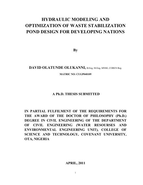
HYDRAULIC MODELING AND 

OPTIMIZATION OF WASTE STABILIZATION 

POND DESIGN FOR DEVELOPING NATIONS 

By 

DAVID OLATUNDE OLUKANNI, B.Eng, M.Eng, MNSE, COREN Reg. 

MATRIC NO: CUGP040109 

A Ph.D. THESIS SUBMITTED 

IN PARTIAL FULFILMENT OF THE REQUIREMENTS FOR 

THE AWARD OF THE DOCTOR OF PHILOSOPHY (Ph.D.) 

DEGREE IN CIVIL ENGINEERING OF THE DEPARTMENT 

OF CIVIL ENGINEERING (WATER RESOURSES AND 

ENVIRONMENTAL ENGINEERING UNIT), COLLEGE OF 

SCIENCE AND TECHNOLOGY, COVENANT UNIVERSITY, 

OTA, NIGERIA 

APRIL, 2011 

i

DECLARATION 

I, Olukanni David Olatunde, declare that this work was done completely by me under the 

supervision of Professor K. O. Adekalu (Main Supervisor) of the Department of 

Agricultural Engineering, Obafemi Awolowo University, Ile-Ife, Osun State, Nigeria and 

Professor J. J. Ducoste (Co-Supervisor) of the Department of Civil, Construction and 

Environmental Engineering, North Carolina State University, Raleigh, North Carolina, 

U.S.A. The thesis has not been presented, either wholly or partly for any degree 

elsewhere. Appropriate acknowledgment has been given where reference has been made 

to the work of others. 

……………………………………… 

Olukanni, D. O. 

ii

CERTIFICATION 

This thesis titled Hydraulic Modeling and Optimization of Waste Stabilization 

Pond Design for Developing Nations carried out by Olukanni, David Olatunde under 

our supervision meets the regulation governing the award of the degree of Doctor of 

Philosophy (Ph.D) in Civil Engineering of the Covenant University, Ota, Ogun State, 

Nigeria. I certify that it has not been submitted for the degree of Ph.D or any other degree 

in this or any other University, and is approved for its contribution to knowledge and 

literary presentation. 

……………………………….. ……………………………… 

Professor K. O. Adekalu Professor. J. J. Ducoste 

(Main Supervisor) (Co-Supervisor) 

……………………………… …………………………… 

Professor J. C. Agunwamba Professor A. S. Adedimila 

(External Examiner) (Head of Department, Civil Engineering) 

iii

DEDICATION 

This thesis is dedicated to my family, Dorcas Eyiyemi (wife), and our son, David 

Olaoluwa Peace, who since birth has been patient and cooperative with us through the 

period of our studies both home and abroad. I love you so much and I know that you are 

the joy to your generation. Remain forever blessed! 

iv

Acknowledgements 

Praise and glory be to the Almighty God from whom all blessings flow. He has enabled 

me to come through to the end of another phase of my educational career. I have received 

numerous help, assistance and guidance from a large number of people over the three 

years that I have worked on this thesis. Of these, I will only be able to mention a few. 

I appreciate my supervisors: Professor Kenneth Adekalu (Obafemi Awolowo University, 

Ile-Ife, Nigeria) and Professor Joel Ducoste (North Carolina State University, Raleigh, 

USA) who find time to scrutinize this work and make useful comments and suggestions. 

Professor Adekalu was instrumental to the course to take at the beginning of this research. 

He prayed alongside with me for the successful award of the Fulbright scholarship while 

Professor Ducoste was very supportive on the CFD models of the laboratory-scale waste 

stabilization ponds that were undertaken. Thank you for the high standard you set for this 

thesis. Without your support and advice, this thesis could not have been produced the way 

it is. The benefits of being able to travel to meet and work with leading researchers around 

the world have been tremendous. 

I wish to express my profound gratitude to the Chancellor, Dr. David Oyedepo for His 

love, support and prayers towards the completion of this program. You have been a 

blessing to me and I will extend this gesture to generations to come. I salute your love for 

God and humanity. 

I also acknowledge the Vice Chancellor of Covenant University, Prof. (Mrs.) Aize 

Obayan, Deputy Vice-Chancellor, Prof. Charles Ogbulogo and the Registrar, Dr. Daniel 

Rotimi for their endless drive and support in making this program a success. Your word of 

encouragement and love has been tremendous. I cannot forget Pastor Yemi Nathaniel, the 

former registrar for his fatherly love and prayers. May God bless you all. 

I appreciate the effort of the former Dean of College of Science and Technology, Prof. 

James Katende for supporting my candidacy for the Fulbright scholarship, without which 

this work would not have been completed. Many thanks to the Dean of Postgraduate 

School and the current Dean of the College of Science and Technology, Prof. C. O. 

Awonuga and Prof. F. K. Hymore for their support to the Postgraduate program at 

v

Covenant University. I am equally grateful to the Head of Department of Civil 

Engineering, Prof. A.S. Adedimila and Prof. J.B. Adeyeri for their efforts towards the 

success of this program. My heartfelt gratitude goes to Prof. K. O. Okonjo and Prof. J. O. 

Bello who gave their time and support to see that this work gets completed in good time. 

My appreciation also goes to the entire staff of my department, both academic and non- 

academic for their contributions towards the successful completion of this study. 

My acknowledgement will be incomplete without mentioning the input of the Department 

of State and Cultural Affairs, United States of America who at the crucial stage of this 

research, awarded me the Fulbright scholarship (administered by Institute of International 

Education) to two universities in United States of America: University of Oklahoma, 

Norman, where I attended a summer intensive study program for 3 months under the 

supervision of Associate Director, Donna Deluca and her entire team. I appreciate your 

love and kindness. The second university I attended was North Carolina State University, 

Raleigh, where I carried out 9 months intensive study and research for the completion of 

my Ph.D thesis. I will not forget to mention my first contact at Raleigh, John and Jean 

Hawes for picking me at the airport and hosting me in their home in Raleigh for few days 

before getting my apartment. These elderly couples are so much appreciated for the love 

and sacrifice shown to me. 

My research work crosses a number of areas: Leslie and Vicky were very helpful in their 

approach to the teaching of technical report writing at the University of Oklahoma. 

Rosario, Sumeet and Chang have been invaluable with regard to setting me up for the 

modeFRONTIER optimization tool. Professors Duncan, Agunwamba and Shilton are 

recognized authority on waste stabilization pond technology. They provided literature 

materials to me that helped in understanding design of the model waste stabilization pond. 

I appreciate you so much. 

I also acknowledged my parents Mr. and Mrs. OLUKANNI for their support in prayers 

and endurance of taking care of our son during the period when my wife and I were 

studying. I thank them for giving me a good foundation in education. I pray that they will 

reap the fruits of their labor abundantly. Amen. I also acknowledge the prayers of my in- 

vi

laws, Mr. and Mrs. BAYODE who call quite often while I was studying abroad. I express 

my gratitude to my immediate family, particularly my wife, Eyiyemi and son, David 

Olaoluwa who supported me while I was away for complete one year in the United States 

of America for the Fulbright program. My gratitude goes to my siblings; Biodun, Bukky, 

Funmi, Wole, Wumi and also my loved ones; Oye, Diran and Olaitan for being part of the 

wonderful family. I appreciate the role of Pastor Mike Ogboluchi at getting the WEST 

software at the beginning of this work and the duo of Dr. Adebayo and Lorenzo Watson 

for their kindness while I was away in the United States of America. 

I sincerely say thank you to all and those whose names have not been able to mention both 

home and abroad who have contributed to the success of this program. God bless you all. 

vii

TABLE OF CONTENTS 

Title page ……………………………………..……………..…............................................i 

Declaration.............................................................................................................................ii 

Certification …………………………….................…………………….....……........…...iii 

Dedication ……………………....……………….……………………….........…...............iv 

Acknowledgements.......……...…….……………………..…………… ….............…….....v 

Table of Contents ………….……………………………………………..……......…......viii 

List of Plates........................................................................................................................xv 

List of Figures ………………….…………………………………………..………........xvi 

List of Tables …...……..………………………………………………............................xxiv 

Abbreviations and symbols...........................................................................................xxvii 

Abstract... …………………...……………………………………………...…….........xxxii 

Chapter 1: 

Introduction…………………………………………………….………………..….…….1 

1.1 Background to the study…….………………….………..….….……...…….…...1 

1.2 Problem statement……………………………………………………………….5 

1.3 Aim of the research………….……………………………...….…….…….….....6 

1.4 Objectives………...…………………..……………………….……….…………6 

1.5 Scope of study……………..………….…………..………....…….....…...……..6 

1.6 Justification of study………………..………….…………………………..…....7 

1.7 Limitation of the work…………………………………………………………..7 

Chapter 2: Literature review………………………………………..……..………….....8 

2.1 The pressure on water demand ………………….….…….…………...……..…..8 

2.2 Wastewater treatment systems in use........…….….…….……..............................9 

2.3 Waste stabilization ponds………………………….………………..……….......11 

viii

2.3.1 Treatment units in Waste Stabilization. Ponds….…………………………....12 

2.3.2 Anaerobic ponds……………………………………………………....……..13 

2.3.2 .1 Design approach for anaerobic pond.........…………………….......…….15 

2.3.3 Facultative ponds……………………………………………………….……17 

2.3.3.1 Design criteria for facultative pond………………………………….…..17 

2.3.3.2 Surface BOD loading in facultative ponds………………………….…...19 

2.3.4 Model approaches for faecal coliform prediction in facultative pond…….......20 

2.3.4.1 Continuous stirred reactor (CSTR) model approach........................….…21 

2.3.4.2 Dispersed flow (DF) model approach……………………………….…..23 

2.3.5 Maturation Pond……………………………………………………………....24 

2.4 Waste Stabilization Ponds in Some Selected Institutions in Nigeria………….…..26 

2.4.1 Waste stabilization pond in University of Nssuka, Nigeria…….…….….29 

2.4.2 Waste stabilization pond in Obafemi Awolowo University, 

Ile-Ife, Nigeria….………………………………………….………......30 

2.4.3 Waste stabilization pond in Ahmadu Bello University, Zaria, 

Nigeria……………………………………………….…………....…...32 

2.5 Residence time-models in waste stabilization ponds ………….………..……....35 

2.5.1 Plug flow pattern…………………………………………..…………......35 

2.5.2 Completely mixed flow pattern………………………….………….…....37 

2.5.3 Dispersed hydraulic flow regime……………………….……………......39 

2.6 Wind effect and thermo-stratification on hydraulic flow regime…………………42 

2.7 Tracer experiment………………………………………………….………………43 

2.8 Effects of baffles on the performance of waste stabilization …….…….……...….44 

2.9 Computational Fluid Dynamics Approach to Waste Stabilization Ponds...............48 

2.10 Laboratory scale ponds……………………………………………….………….56 

2.11 Optimization of waste stabilization pond design…………………….…………..59 

2.12 Summary of literature review……………………………………….….………...61 

Chapter 3: 

Methodology….……………………………………….…………..………….......….....62 

3.1 Description of the study area……………….…………………………..………..62 

ix

3.2 Collection of data on Water demand…………………………….……….…….....65 

3.3 Estimation of wastewater generated ………………………….…….…….…..…..66 

3.4 Study of existing wastewater treatment system……….……..…..……….………66 

3.5 Analysis of wastewater samples…………………….….………..….….………....70 

3.6 Design of the laboratory-scale plant layout……………….….…….…………......70 

3.6.1. Design Guidelines for the University, Ota……..………….……..……..73 

3.6.1.1 Temperature (T)…………………….….………….……….……73 

3.6.1.2 Population (P)……………………….…………..………….…...73 

3.6.1.3 Wastewater generation (Q) and Design for 20 years period........73 

3.6.1.4 BOD Contribution per capita per day (BOD)………………..…73 

3.6.1.5 Total Organic Load (B)……………………….…….…………..74 

3.6.1.6 Total Influent BOD Concentration (Li)…….……….….....……..74 

3.6.1.7 Volumetric organic loading (λv) ……………………..…….......74 

3.6.1.8 Influent Bacteria Concentration (Bi)………………….………..74 

3.6.1.9 Required effluent standards………..………………….…….....74 

3.7 Waste stabilization pond design……..……………………………….....….…......75 

3.7.1 Design of Anaerobic Pond. ……………………….…………….…..……75 

3.7.2 Design of Facultative pond…………………….………….…….….........76 

3.7.3 Design of Maturation Pond…………………….……………….…..........77 

3.8 Design of Laboratory scale model............................................................................79 

3.8.1 Modeling of the Anaerobic Laboratory-scale pond.. ………………........79 

3.8.2 Modeling of the Facultative Laboratory-scale pond……..……..…..........81 

3.8.3 Modeling of the Maturation Laboratory-scale pond..……..…….…….....82 

3.9 Laboratory Studies………..……..…………………………......…………………...85 

3.9.1 Construction of the laboratory-scale waste stabilization ponds….….…...85 

3.9.2 Materials used for the construction of the inlet and outlet structures…....86 

3.9.3 Design of inlet and outlet structures of the WSP………..…………….....91 

3.9.4 Operation of the Laboratory-Scale waste stabilization pond………........94 

3.9.5 Sampling and data collection……………………………………………95 

3.9.5.1 Water temperature………………………………………………….95 

3.9.5.2 Influent and effluent samples………………………………………95 

x

3.10 Laboratory methods ………….…………………..……………..……….……….95 

3.10.1 Feacal coliform………………………….……………..…………..….....96 

3.10.2 Chloride………………………………………….………………..……..96 

3.10.3 Sulphate…………………………………..…………..……………..…..96 

3.10.4 Nitrate…………………………….……..………….……….…….….....96 

3.10.5 Phosphate…………………………………...……………………...…....96 

3.10.6 Total Dissolved Solids..………………………………………….….…...96 

3.10.7 Conductivity..……………………………………………...………..…...97 

3.10.8 pH……………….…………..…………..…………………………..… ..97 

3.11 Tracer Experiment……………….….……...…………….………………….… ....97 

3.11.1 Determination of First Order Kinetics (K value) for Residence time 

distribution (RTD) characterization.….……………………………..… ..99 

3.11.2 The gamma extension to the N-tanks in series model approach.….... 101 

3.12 Methodology and application of Computational Fluid Dynamics model…....… 103 

3.12.1 Introduction…………………………………………..…………….…. ..103 

3.12.2 CFD Model Application ……………………….….……………….….. .106 

3.12.2.1 Simulation of fluid mechanics fecal coliform inactivation…… 106 

3.12.2.2 Constants used in the application modes………………………109 

3.12.2.3 Mesh generation for the computational fluid dynamics model..110 

3.12.2.4 Model test for the simulation of residence time distribution 

curve in the CFD……………………………………………...113 

3.12.2.5 Model test for the simulation of faecal coliform inactivation in 

the unbaffled reactor…..………….………..….……………...114 

3.12.2.6 Model test for the simulation of faecal coliform inactivation in 

the baffled reactors…………………………………………….116 

3.12.3 Application of segregated flow model to compare RTD prediction 

and the CFD predictions for feacal coliform reduction……………..…122 

3.12.4 Summary of the CFD model methodology…..……………….........…..124 

3.13.1 Optimization methodology and application..………..….……………………125 

3.13.1.1 Integration of COMSOL Multiphysics (CFD) with 

ModeFRONTIER optimization tool……..………….….…..….…...125 

xi

3.13.1.2 The workflow pattern............................................................................126 

3.13.1.3 Building the process flow......................................................................127 

3.13.1.4 Creating the application script...............................................................128 

3.13.1.5 Creating the data flow...........................................................................129 

3.13.1.6 Creating the template input...................................................................130 

3.13.1.7 Mining the output variables from the output files.................................131 

3.13.2 Defining the goals..................................................................................................132 

3.13.2.1 The Objective functions for the optimization loop….…..…..………...132 

3.13.2.2 The constraints for the optimization loop………….……...….……….133 

3.13.2.3 Cost objective Optimization ……………………….……...….……....133 

3.13.2.4 The DOE and scheduler nodes set up....................................................136 

3.13.2.5 Model parameterization of input variables …………….…..….……...137 

3.13.2.6 DOE Algorithm…………………………………………….……...….….......140 

3.13.2.7 Simplex algorithm………..…………………………………...…...….....140 

3.13.2.8 Multi-Objective Genetic Algorithm II (MOGA-II) ….......…................141 

3.13.2.9 Faecal coliform log-removal for transverse and longitudinal 

baffle arrangements………….…...………………………….……..….143 

3.13.3 Sensitivity Analysis on the model parameters………..……………..…..…….145 

3.13.4 Running of output results from modeFRONTIER with the CFD tool….…...……....146 

3.13.5 Summary of the optimization methodology………………………….…......….…....146 

Chapter 4: Modeling results and Analysis 

4.1 Model results for the RTD curve and FC inactivation for unbaffled reactors…..147 

4.2 Initial Evaluation of baffled WSP designs in the absence of Cost using CFD.…151 

4.2.1 Application of segregated flow model to compare the result of RTD 

prediction and the CFD predictions for feacal coliform reduction….……..163 

4.3 Results of the N-Tanks in series and CFD models …………………...….….......166 

4.3.1 General discussion on the results of the N-Tanks in series and CFD 

Models……………………………………………………………………....173 

4.4 Results of some selected simulation of faecal coliform inactivation for 80% 

Pond-width baffle Laboratory- scale reactors……………………………….....176 

xii

4.5 Optimization model results………………….…………….…………….……........181 

4.5.1 The single objective SIMPLEX optimization configuration results………...181 

4.5.2 The Multi-objective MOGA II optimization configuration results………....195 

4.5.3 Scaling up of Optimized design configuration………………………….…..216 

4.5.3.1 Scaling up of Anaerobic Longitudinal baffle arrangement…….......216 

4.5.3.2 Scaling up of Facultative Transverse baffle arrangement……….....218 

4.5.3.3 Scaling up of Maturation Longitudinal baffle arrangement………..219 

4.5.3.4 Summary of results of scaling up of design configuration…….…....220 

4.5.4 Results of sensitivity analysis for Simplex design at upper and lower 

boundary……………….…………………………………………….……..220 

4.5.5 Results of sensitivity analysis for MOGA II design at upper and lower 

boundary…………………………………………………….…..…........235 

4.5.6 Summary of the optimization model result.………………………..…..........249 

Chapter 5: Laboratory-Scale WSP post-modeling results and verification of the 

Optimized models………………………………………………..……..250 

5.1 Introduction………………………………………………………………..…….250 

5.2 Microbial and physico-chemical parameters……………………………..………251 

5.2.1 Feacal coliform inactivation in the reactors………………………..…….....251 

5.2.2 Phosphate removal………………………………………………..………...256 

5.2.3 Chloride removal…………………………………………….……………..258 

5.2.4 Nitrate removal……………………………………………….…………….259 

5.2.5 Sulphate removal…………………………………………….……………..260 

5.2.6 pH variation………………………………………………….……………..265 

5.2.7 Total dissolved solids removal…………………………….……………….266 

5.2.8 Conductivity variation…………………………………….………………..266 

5.2.9 Summary of laboratory experimentation………………….………………..267 

Chapter 6: Discussion of results……………………….………………………….269 

6.1 Experimental results of Laboratory-scale waste stabilization ponds 

in series…....................................................................................................269 

xiii

6.2 Hydraulic efficiency of CFD model laboratory-scale waste stabilization 

ponds in series..……………………….……….………………………..…270 

6.3 Optimization of laboratory-scale ponds by Simplex and MOGA II 

Algorithms………………………….………………………………….......274 

6.4 Summary of discussion…………………………………………………....275 

Chapter 7: Conclusions and recommendations for further work…….….….…277 

7.1 Conclusions…………………………………………………….…….……277 

7.2 Contributions to knowledge………………………………………………278 

7.3 Recommendation for further work…………………………….….…..…..279 

References………………………………………………………………………....280 

Appendix A………………………………………………………..……………....298 

A1 COMSOL Multiphysics Model M-file for Transverse baffle 

anaerobic reactor………………………..……………………………,…......298 

A2 COMSOL Multiphysics Model M-file for longitudinal baffle 

anaerobic reactor………………………….…..…………………………......302 

A3 COMSOL Multiphysics Model M-file for Transverse baffle 

facultative reactor………………………………………...…………...……306 

A4 COMSOL Multiphysics Model M-file for longitudinal baffle 

facultative reactor……………………………………………..…………..310 

A5 COMSOL Multiphysics Model M-file for Transverse 

Maturation reactor…………………………………………………………..314 

A6 COMSOL Multiphysics Model M-file for longitudinal 

Maturation reactor………………………………………………………….318 

Appendix B………………………………………………………………………322 

B1 Transverse baffle arrangement scripting…………………………………...322 

B2 Longitudinal baffle arrangement scripting…………………………………324 

xiv

List of Plates 

Plate 3.1 Tanker dislodging wastewater into the treatment chamber….….….………67 

Plate 3.2 The water hyacinth reed beds showing baffle arrangement 

at opposing edges…………………………………………….…….……...68 

Plate 3.3 The inlet compartment showing gate valve…………………….….………68 

Plate 3.4 The Outfall waterway leading into the valley below the cliff…….….……69 

Plate 3.5 Effluent discharging through the outfall into the thick 

vegetation valley…………………………………………………….….….69 

Plate 3.6 Front view of the laboratory-scale pond.......................................................88 

Plate 3.7 Areal view of the laboratory-scale pond close to source of sunlight...........88 

Plate 3.8 An elevated tank serving as reservoir..........................................................89 

Plate 3.9 Inlet-outlet alternation of laboratory-scale WSP…………………….……89 

Plate 3.10 Laboratory-scaled anaerobic ponds………………………………………90 

Plate 3.11 Laboratory-scaled facultative ponds……………………………………...90 

Plate 3.12 Laboratory-scaled maturation ponds…………………………………......91 

Plate 3.13 Inlet and outlet structure of the laboratory-scale 

waste stabilization pond…………………………………………………92 

Plate 3.14 Two 25-mm PVC hoses linked with the T-connector………………….....92 

Plate 3.15 Control valves screwed to position for wastewater flow…………………93 

Plate 3.16 Outlet structures connected to two pieces of ½ inch hoses 

for effluent Discharge…………………………………………….……….93 

Plate 3.17 Tracer experiment with Sodium Aluminum Sulphosilicate…….……......97 

Plate 3.18 Tracer chemical diluting with the wastewater before 

getting to the outlet………………………………………………….…....98 

Plate 3.19 Improvement in wastewater quality along the units…………….…….....98 

xv

List of Figures 

Figure 2.1 Waste stabilization pond configurations 12 

Figure 2.2 Operation of the Anaerobic Pond 14 

Figure 2.3 Operation of the facultative pond 23 

Figure 3.1 Bar chart of staff and student population trend 63 

Figure 3.2 Template for calculating the per-capita water use 65 

Figure 3.3 A sketch of the laboratory-scale WSP and operating conditions 72 

Figure 3.4 Configuration of the designed WSP for Covenant University 79 

Figure 3.5 Different baffle arrangements with 70% pond width 

anaerobic pond 99 


facultative pond 100 


maturation pond 100 

Figure 3.8 Data conversion for reactor length to width ratio to N for 

N-tanks in series model 102 

Figure 3.9 Description of length to width ratio for the laboratory-scale 

model 102 

Figure 3.10 Triangular meshes for the model anaerobic reactor 111 

Figure 3.11 Triangular meshes for the model facultative reactor 111 

Figure 3.12 Triangular meshes for the model maturation reactor 112 

Figure 3.13 Model Navigator showing the application modes 113 

Figure 3.14 Correlation data of the predicted-CFD and observed effluent Faecal 

coliform counts in baffled pilot-scale ponds 115 

Figure 3.15 General arrangements of conventional longitudinal baffles of 

different lengths in the anaerobic pond 117 


different lengths in the facultative pond 117 


different lengths in the maturation pond 118 

xvi

Figure 3.18 Mesh structure in a 4 baffled 70% Transverse Anaerobic reactor 118 

Figure 3.19 Mesh structure in a 4 baffled 70% Longitudinal Anaerobic reactor 119 

Figure 3.20 Mesh structure in a 4 baffled 70% Transverse Facultative 119 

Figure 3.21 Mesh structure in a 4 baffled 70% Longitudinal Facultative 

reactor 120 

Figure 3.22 Mesh structure in a 4 baffled 70% Transverse Maturation 

reactor 120 

Figure 3.23 Mesh structure in a 4 baffled 70% Longitudinal Maturation 

reactor 121 

Figure 3.24 Workflow showing all links and nodes in the user application 

interface 127 

Figure 3.25 Logic End properties dialogue interface 128 

Figure 3.26 Data variable carrying nodes and the input variable properties 

Dialogue interface 129 

Figure 3.27 Template for the calculator properties and JavaScript 

expression editor 130 

Figure 3.28 Output variable mining interface and input template editor 131 

Figure 3.29 DOS Batch properties and batch test editor for mined data 132 

Figure 3.30 Constraint properties dialogue in the workflow canvas 135 

Figure 3.31 Objective properties dialogue in the workflow canvas 135 

Figure 3.32 DOE properties dialog showing the initial population of designs 136 

Figure 3.33 Scheduler properties dialog showing optimization wizards 137 

Figure 3.34 Designs table showing the outcomes of different reactor 

configurations 144 

Figure 3.35 History cost on designs table showing the optimized cost 144 

Figure 4.1 Residence time distribution curve for unbaffled anaerobic reactor 148 

Figure 4.2 Anaerobic unbaffled reactor coliform inactivation 148 

Figure 4.3 Residence time distribution curve for unbaffled facultative reactor 149 

Figure 4.4 Facultative unbaffled reactor coliform inactivation 149 

Figure 4.5 Residence time distribution curve for unbaffled maturation reactor 150 

Figure 4.6 Maturation unbaffled reactor coliform inactivation 150 

xvii

Figure 4.7 Overall log reductions for the WSP system over a range of baffle lengths 154 

Figure 4.8 Residence time distribution curve for transverse 4-baffle 70% 

anaerobic reactor 157 

Figure 4.9 Velocity streamline and coliform inactivation for transverse 4 baffles 

70% pond width anaerobic reactor 157 


Facultative reactor 158 

Figure 4.11 Velocity streamline and coliform inactivation for transverse 4 baffle 70% 

pond width facultative reactor 158 


Maturation reactor 159 

Figure 4.13 Velocity streamline and coliform inactivation for transverse 4 baffle 70% 

pond width Maturation reactor 159 

Figure 4.14 Residence time distribution curve for longitudinal 4-baffle 70% 

Anaerobic reactor 160 

Figure 4.15 Velocity streamline and coliform inactivation for longitudinal 70% pond 

width anaerobic reactor 160 


Facultative reactor 161 

Figure 4.17 Velocity streamline and coliform inactivation for longitudinal 4 baffle 

70% pond width facultative reactor 161 


Maturation reactor 162 

Figure 4.19 Velocity streamline and coliform inactivation for transverse anaerobic 

Reactor 162 

Figure 4.20 Comparion between CFD model and N-tanks in series residence time 

density curves for 2 baffles 70% pond width Facultative reactor 167 

xviii






density curves for 2 baffles 70% pond width Maturation reactor 169 






density curves for 2 baffles 80% pond width facultative reactor 170 











Figure 4.32 Faecal coliform inactivation in a longitudinal 4-baffle 80% pond width 


Figure 4.33 Faecal coliform inactivation in a transverse 6-baffle 80% pond width 



facultative reactor 178 



xix




maturation reactor 179 

Figure 4.38 SIMPLEX history cost on design for the combination of even and odd 

Transverse baffle arrangement in anaerobic reactor 182 

Figure 4.39 SIMPLEX optimal faecal coliform removal design with least 

cost for transverse baffle arrangement in anaerobic reactor 184 

Figure 4.40 SIMPLEX maximum faecal coliform removal design for 

transverse baffle arrangement in anaerobic reactor 185 

Figure 4.41 SIMPLEX optimal faecal coliform removal design with least cost 

for transverse baffle arrangemnt in facultative reactor 186 


for transverse baffle arrangement in maturation reactor 187 

Figure 4.43 SIMPLEX history cost on design for longitudinal baffle arrangement 

in anaerobic reactor 188 


longitudinal baffle arrangement in anaerobic reactor 190 

Figure 4.45 SIMPLEX minimum faecal coliform removal design for 

Longitudinal baffle arrangement in anaerobic reactor 191 

Figure 4.46 SIMPLEX optimal faecal coliform removal design for 

longitudinal baffle arrangement in facultative reactor 192 

Figure 4.47 SIMPLEX minimum faecal coliform removal design for 

longitudinal baffle arrangement in facultative 193 

Figure 4.48 MOGA-II history costs on design for even transverse baffle 

arrangement in anaerobic reactor 195 

Figure 4.49 MOGA-II history cost on design for transverse baffle 

arrangement in facultative reactor 196 

Figure 4.50 MOGA-II history costs on design for transverse baffle arrangement 

in maturation reactor 197 

Figure 4.51 Trade off plot for Anaerobic Transverse design space 198 

xx

Figure 4.52 Trade off plot for Facultative Transverse design space 199 

Figure 4.53 Trade off plot for Maturation Transverse design space 200 

Figure 4.54 MOGA-II optimal faecal coliform removal design with least cost 

for even baffle transverse arrangement in anaerobic reactor 202 

Figure 4.55 MOGA-II maximum faecal coliform removal design for even baffle 

transverse arrangement in anaerobic reactor 203 


for even baffle transverse arrangement in facultative reactor 204 


for even baffle transverse arrangement in maturation reactor 205 


transverse arrangement in maturation reactor 206 

Figure 4.59 Trade off plot for anaerobic longitudinal design space 207 

Figure 4.60 Trade off plot for facultative longitudinal design space 208 

Figure 4.61 Trade off plot for maturation longitudinal design space 209 


for even baffle longitudinal arrangement in anaerobic reactor 211 


for even baffle longitudinal arrangement in facultative reactor 212 

Figure 4.64 MOGA-II maximum faecal coliform removal design for even 

baffle longitudinal arrangement in facultative reactor 213 


for even baffle longitudinal arrangement in maturation reactor 214 


for transverse baffle arrangement in anaerobic reactor (k = 13.686) 222 

Figure 4.67 SIMPLEX sensitivity optimal faecal coliform removal design for 

transverse baffle arrangement in facultative reactor (k = 13.686) 222 


transverse baffle arrangement in maturation reactor (K= 13.686) 223 


longitudinal baffle arrangement in anaerobic reactor (k = 13.686) 225 

xxi


longitudinal baffle arrangement in facultative reactor (k = 13.686) 225 


longitudinal baffle arrangement in maturation reactor (k = 13.686) 226 


transverse baffle arrangement in anaerobic reactor (k = 4.562) 229 


transverse baffle arrangement in facultative reactor (k = 4.562) 229 


transverse baffle arrangement in maturation reactor (k = 4.562) 230 


longitudinal baffle arrangement in anaerobic reactor (k = 4.562) 232 


longitudinal baffle arrangement in facultative reactor (k = 4.562) 232 


longitudinal baffle arrangement in maturation reactor (k = 4.562) 233 

Figure 4.78 MOGA II sensitivity analysis optimal faecal coliform removal design 

for transverse baffle arrangement in anaerobic reactor (k = 13.686) 236 


for transverse baffle arrangement in facultative reactor (k = 13.686) 236 


for transverse baffle arrangement in maturation reactor (k = 13.686) 237 


for longitudinal baffle arrangement in anaerobic reactor (k = 13.686) 239 


for longitudinal baffle arrangement in facultative reactor (k = 13.686) 239 


for longitudinal baffle arrangement in maturation reactor (k = 13.686) 240 


for transverse baffle arrangement in anaerobic reactor ( k = 4.562) 243 

xxii


for transverse baffle arrangement in facultative reactor (k = 4.562) 243 


for transverse baffle arrangement in maturation reactor (k = 4.562) 244 


for longitudinal baffle arrangement in anaerobic reactor (k= 4.562) 246 


for longitudinal baffle arrangement in facultative reactor (k = 4.562) 246 


for longitudinal baffle arrangement in maturation reactor (k = 4.562) 247 

Figure 5.1 Different tested laboratory-scale reactor configuration 252 

Figure 5.2 Laboratory effluents sampling during the experiment 252 

xxiii

List of Tables 

Table 2.1 Important factors in the selection of wastewater treatment systems 

in developed and developing countries 9 

Table 2.2 Advantages and disadvantages of various sewage treatment systems 10 

Table 2.3 Typical Dimensions and configurations of some Waste Stabilization 

Pond in Nigeria 28 

Table 2.4 Summary of engineering properties and physical assessment at 

ABU, Zaria 33 

Table 2.5 Summary of the assessment at ABU, Zaria 34 

Table 2.6 Classification of wastewater based on composition 34 

Table 3.1 Student Population Trend in Covenant University since Inception 63 

Table 3.2 Dimensions of laboratory scale models of WSP 84 

Table 3.3 Mesh statistics for the unbaffled laboratory-scale pond models 112 

Table 3.4 Mesh statistics for 4-baffled laboratory-scale pond models 121 

Table 3.5 Range of adjusted parameter values 134 

Table 3.6 Scheduler based on Multi Objective Algorithm (MOGA-II) 

Design table 142 

Table 4.1 Results of different simulated configurations using the CFD model 153 

Table 4.2 CFD Results and associated costs for 70% pond-width Transverse 

baffle arrangement 155 

Table 4.3 CFD Results and associated costs for 70% pond-width Longitudinal 

baffle arrangement 156 

Table 4.4 Actual simulated hydraulic retention time (in days) for the three 

reactors 164 

Table 4.5 Comparison of the RTD and the CFD predictions for feacal coliform 

Reduction 165 

Table 4.6 Laboratory system geometry and flow rate conditions in published 

literature 175 

Table 4.7: Laboratory-scale system geometry and flow rate conditions in 

this study 175 

xxiv

Table 4.8 SIMPLEX designs for transverse baffle arrangement 183 

Table 4.9 SIMPLEX designs for longitudinal baffle arrangement 189 

Table 4.10 Simplex Optimal design results 194 

Table 4.11 MOGA-II designs for transverse baffle arrangement 201 

Table 4.12 MOGA-II designs for longitudinal baffle arrangement 210 

Table 4.13 MOGA-II Optimal design results 215 

Table 4.14 Summary of results of scaling up of design configuration 220 

Table 4.15 Sensitivity Analysis Results for Transverse baffle arrangement 

(k =13.686) 221 

Table 4.16 Simplex Sensitivity Analysis Results for Longitudinal baffle 

arrangement (k =13.686) 224 

Table 4.17 SIMPLEX sensitivity analysis optimal design results for k = 13.686 227 

Table 4.18 Sensitivity Analysis Results for Transverse baffle arrangement 

(k = 4.56) 228 

Table 4.19 Sensitivity Analysis Results for Longitudinal baffle arrangement 

(k= 4.562) 231 

Table 4.20 SIMPLEX sensitivity analysis optimal design results for k = 4.562 234 

Table 4.21 MOGA-II Sensitivity Analysis Results for Transverse baffle 

(k= 13.686) 235 

Table 4.22 MOGA-II Sensitivity Analysis Results for Longitudinal arrangement 

(k = 13.686) 238 

Table 4.23 MOGA-II Sensitivity Analysis Optimal Design Results k = 13.686 241 

Table 4.24 MOGA-II Sensitivity Analysis Results for Transverse arrangement 

(k = 4.562) 242 

Table 4.25 MOGA-II Sensitivity Analysis Results for Longitudinal arrangement 

(k= 4.56) 245 

Table 4.26 MOGA-II Sensitivity Analysis Optimal Design Results k = 4.562 248 

Table 5.1 Experimental data of feacal coliform inactivation in the reactors 253 

Table 5.2 Experimental data of Phosphate removal for all the reactor configurations 257 

Table 5.3 Experimental data of Chloride removal for all the reactor configurations 258 

Table 5.4 Experimental data of Nitrate removal for all the reactor configurations 259 

xxv

Table 5.5 Experimental data of Sulphate removal for the reactor configurations 260 

Table 5.6 Experimental data of nutrient removal for the anaerobic reactor 

Configurations 262 

Table 5.7 Experimental data of nutrient removal for the facultative reactor 

Configurations 263 

Table 5.8 Experimental data of Sulphate removal for the reactor configurations 264 

Table 5.9 Experimental data of PH variation for all the reactor configurations 265 

Table 5.10 Experimental data of TDS removal for all the reactor configurations 266 

Table 5.11 Conductivity experimental data for all the reactor configurations 267 

Table 6.1 Reported values of B( 

20 ) 

k and φ in the first-order rate constant 

removal equation of faecal coliform in waste stabilization ponds 270 

xxvi

Abbreviations and Symbols 

ABU Ahmadu Bello University, Zaria 

APHA American Public Health Association 

ASCII American Standard Code for Information Interchange 

ASS Atomic Absorption Spectrophotometry 

Af area of facultative pond/reactor 

Am area of maturation pond/reactor 

BOD5 biochemical oxygen demand for 5 days 

Be number of FC/100ml of effluent 

Bi number of FC/100ml of influent 

c tracer concentration 

CEC cation exchange capacity 

CFD computational fluid dynamics 

CLMT Canaan Land Mass Transit 

COD chemical oxygen demand 

CSTR complete stared treatment reactor 

DOS disk operating system 

DO dissolved oxygen 

DOE design of experiment 

Di diffusion coefficient 

Da depth of anaerobic pond/reactor 

Df depth of facultative pond/reactor 

Dm depth of maturation pond/reactor 

DF dispersed flow 

xxvii

d dispersion number 

dx,dy,dz differential change in distance 

dt differential change in time 

D coefficient of longitudinal dispersion 

E eddy viscosity coefficient 

FC faecal coliform 

F volume force in the x and y direction 

FEPA Federal Environmental Protection Agency 

Fr Froude number 

g acceleration due to gravity 

GA genetic algorithm 

H 2 S hydrogen sulphide gas 

HRT hydraulic retention time 

JAMB joint admission and matriculation board 

KB(T) first-order rate constant removal of pollutant at temperature T 

K1(20) first-order rate constant removal of pollutant at temperature T 

K BODP BOD removal constant rate in the plug flow pond model 

KBOD D BOD removal constant rate in the dispersed flow pond model 

KBOD C completely mixed first-order rate constant for BOD removal 

Le effluent BOD5 concentration 

Li influent BOD5 concentration 

l length of flow path 

L pond length 

Lo baffle opening 

Lr Scale ratio 

xxviii

MOGA multi-objective genetic algorithm 

NH3-N Ammonia- nitrogen 

OAU Obafemi Awolowo University, Ile-Ife, Nigeria 

p pressure 

pH activity of hydrogen ions = log10(hydrogen ion concentrations) 

POTW public owned treatment works 

PPDU physical planning and development unit 

PVC polyvinyl chloride 

Qm waste water flow rate in model 

Qp waste water flow rate in prototype 

Q mean design wastewater flow 

Q r recycled flow rate 

RBC rotating biological contactors 

R(c) rainfall/evaporation rate. 

R 2 coefficient of correlation 

Re Reynolds number 

RTD residence time distribution 

Sφ source term of scalar variable φ 

SO4 sulphate 

SS suspended solids 

SSE sum of squares of errors 

SL scaling factor 

T temperature 

t time taken by tracer from the inlet to outlet 

t* retention time in any pond 

xxix

TN Total Nitrogen 

t mean hydraulic retention time obtained from tracer 

experiments 

TSS total suspended solid 

UN United Nations 

USA United States of America 

USEPA United State Environmental Protection Agency 

USAID United States Agency for International Development 

UDF user defined function 

UNN University of Nigeria, Nssuka 

u velocity 

UASB upflow anaerobic sludge blanket 

u,v,w velocity in x,y and z directions 

UV ultraviolet radiation 

Vm velocity of model 

Vp velocity of prototype 

WW wastewater 

w baffle spacing, pond width 

WA Western Australia 

WHO World Health Organization 

WSP waste stabilization pond 

WWTP wastewater treatment plant 

θ theoretical hydraulic retention time 

λ s 

surface BOD loading 

λ v 

volumetric organic loading rate 

xxx

0 C degree Celsius 

∞ infinity 

ρ wastewater density 

µ dynamic viscosity 

φ scalar variable 

σ source/ sink of constituent 

2D two dimensional 

3D three dimensional 

Γ gamma function 

ξ empirical wind shear coefficient 

ψ wind direction 

ω rate of earth`s angular rotation 

ϕ local latitude 

η dynamic viscosity 

δ st 

time-scaling coefficient 

υ kinematic viscosity 

xxxi

ABSTRACT 

Wastewater stabilization ponds (WSPs) have been identified and are used extensively to 

provide wastewater treatment throughout the world. It is often preferred to the 

conventional treatment systems due to its higher performance in terms of pathogen 

removal, its low maintenance and operational cost. A review of the literature revealed that 

there has been limited understanding on the fact that the hydraulics of waste stabilization 

ponds is critical to their optimization. The research in this area has been relatively limited 

and there is an inadequate understanding of the flow behavior that exists within these 

systems. This work therefore focuses on the hydraulic study of a laboratory-scale model 

WSP, operated under a controlled environment using computational fluid dynamics (CFD) 

modelling and an identified optimization tools for WSP. 

A field scale prototype pond was designed for wastewater treatment using a typical 

residential institution as a case study. This was reduced to a laboratory-scale model using 

dimensional analysis. The laboratory-scale model was constructed and experiments were 

run on them using the wastewater taken from the university wastewater treatment facility. 

The study utilized Computational Fluid Dynamics (CFD) coupled with an optimization 

program to efficiently optimize the selection of the best WSP configuration that satisfy 

specific minimum cost objective without jeopardizing the treatment efficiency. This was 

done to assess realistically the hydraulic performance and treatment efficiency of scaled 

WSP under the effect of varying ponds configuration, number of baffles and length to 

width ratio. Six different configurations including the optimized designs were tested in the 

laboratory to determine the effect of baffles and pond configurations on the effluent 

characteristics. The verification of the CFD model was based on faecal coliform 

inactivation and other pollutant removal that was obtained from the experimental data. 

The results of faecal coliform concentration at the outlets showed that the conventional 

70% pond-width baffles is not always the best pond configuration as previously reported 

in the literature. Several other designs generated by the optimization tool shows that both 

shorter and longer baffles ranging between 49% and 83% for both single and multiobjective 

optimizations could improve the hydraulic efficiency of the ponds with different 

variation in depths and pond sizes. The inclusion of odd and even longitudinal baffle 

arrangement which has not been previously reported shows that this configuration could 

improve the hydraulic performance of WSP. A sensitivity analysis was performed on the 

model parameters to determine the influence of first order constant (k) and temperature 

(T) on the design configurations. The results obtained from the optimization algorithm 

considering all the parameters showed that changing the two parameters had effect on the 

effluent faecal coliform and the entire pond configurations. 

This work has verified its use to the extent that it can be realistically applied for the 

efficient assessment of alternative baffle, inlet and outlet configurations, thereby, 

addressing a major knowledge gap in waste stabilization pond design. The significance of 

CFD model results is that water and wastewater design engineers and regulators can use 

CFD to reasonably assess the hydraulic performance in order to reduce significantly faecal 

coliform concentrations and other wastewater pollutants to achieve the required level of 

pathogen reduction for either restricted or unrestricted crop irrigation. 

xxxii

CHAPTER ONE 

INTRODUCTION 

1.1 Background to the Study. 

The practice of collecting, treating and proper management of wastewater prior to disposal 

has become a necessity in developing and modern societies. This is because the 

consequences due to poor management of wastewater treatment systems have become 

enormous. Moreover, the need to minimize waste and make the most valuable use of 

nutrients present in wastewater is receiving global interest. Bixio et al. (2005) pointed out 

that the world’s freshwater resources are strained; therefore, reuse of wastewater, 

combined with other water conservation strategies can lessen anthropogenic stress arising 

from over-extraction and pollution of receiving waters. 

As reported by the World Health Organization (2000), “despite tremendous efforts in the 

last two decades to provide improved water and sanitation services for the poor in the 

developing world, 2.4 billion people world-wide still do not have any acceptable means of 

sanitation, while 1.1 billion people do not have an improved water supply”. This indicates 

that less than 1% and 15% of the wastewaters collected in sewered cities and towns in 

Africa and Latin America, respectively, are treated in effective sewage treatment plants. 

Mara (2001) also reported that out of the world population of just over 6 billion, 4 billion 

lack wastewater treatment and this is expected to rise to 7.8 billion by 2025. Most of these 

live in developing countries where energy-intensive electro-mechanical wastewater 

treatment (the type favoured in industrialized countries) is too expensive and too difficult 

to operate and maintain. 

Wastewater is the water that has been adversely affected in quality by anthropogenic 

influence. It comprises liquid waste discarded by domestic residences, commercial 

properties, industry, and/or agriculture. Banda (2007) emphasized the significant 

composition of wastewater as the degradable organic compounds and these form an 

1

excellent diet for bacteria and are exploited in biological treatment of wastewater. In order 

to reduce the transmission of the excreta-related diseases and the damage to aquatic biota, 

Mara (2004) express the necessity to treat wastewater to meet the consent requirements of 

the effluent quality set by the regulatory agencies. 

The safe disposal of wastewater has been a great concern in developing nations, most 

especially in Nigeria. In 2008, estimated population of Nigeria was 151.5 million (UN, 

2008) yielding an average density of 151 persons per sq km covering an area of 923,768 

sq km (356,669 sq miles). The population is projected to grow to 206 million by 2025 

(Microsoft Encarta Encyclopedia, 2005). Treatment ponds serve thousands of 

communities around the world. In many cases, they are the only form of environmental 

protection that stands between raw sewage and natural waterways. Unfortunately, 

ignorance and lack of knowledge are responsible for poor wastewater treatment in many 

of these nations (Mara, 2004). 

Among the current, globally available processes used for wastewater treatment, waste 

stabilization pond (WSP) has been identified as the ideal treatment of municipal 

wastewaters in the tropics. This technology is well known for its simplicity of construction 

and operation (Mara, 2004). Shilton and Bailey (2006) noted that the only thing standing 

between raw sewage and the environment, into which it is ultimately discharged, is a 

waste stabilization pond. WSP has been emphasized to be the first choice wastewater 

treatment facilities in developing countries as these operate extremely well in tropical 

regions at low-cost (Mara et al. 1992; Mara, 1997; Mara and Pearson, 1998). The WSP 

system typically consists of a series of continuous flow anaerobic, facultative, and 

maturation ponds. The anaerobic pond, which is the initial treatment reactor, is designed 

for eliminating suspended solids and some of the soluble organic matter. The residual 

organic matter is further removed through the activity of algae and heterotrophic bacteria 

in the facultative pond. The final stage of pathogens and nutrients removal takes place in 

the maturation pond. These three types of ponds when used in series, have demonstrated 

up to 95% removal of BOD and fecal coliform. (Mara, 2004; Hamzeh and Ponce, 2007). 

2

In Nigeria, WSPs have been installed in some universities for domestic wastewater 

treatment. From preliminary investigation, the design population for most of these 

Nigerian ponds has been exceeded and has lead to serious overloading problems from 

deficient hydraulic designs (Agunwamba, 1994 and 2001; Oke and Akindahunsi, 2005; 

Olukanni and Aremu, 2008). Despite abundant lands, large surface area ponds and 

favourable temperatures, the waste stabilization ponds are not able to produce treated 

effluents that meet the minimum standard limits set by Nigeria’s Federal Environmental 

Protection Agency (FEPA, 1991). Most waste stabilization ponds in residential academic 

institutions discharge their effluents into the environment without adequate treatment 

which cause great negative impact on the aquatic life of the receiving streams. 

Research is therefore needed to address the weakness in the pond`s treatment capacity. It 

is believed that processes exist within ponds that, if understood better, could be optimized 

to enable effective treatment of wastewater with limited cost of construction and 

maintenance. This is the main focus of the research project. Previous studies have shown 

that the WSP treatment efficiency is often hydraulically compromised (Shilton and Mara, 

2005; Shilton and Harrison 2003a). The majority of the hydraulic studies on WSPs have 

been performed on full-scale field ponds, which have transient flows and large surface 

areas exposed to wind and temperature variations (Marecos and Mara, 1987; Moreno, 

1990; Agunwamba, 1992; Fredrick and Lloyd, 1996; Adewumi et al, 2005). 

Researchers have been challenged to reliably predict the impact of pond design 

modifications, such as placement and number of baffles and different flow rates on the 

pond performance using field scale WSPs. Antonini et al., (1983) and later Shilton and 

Bailey (2006) noted that operation and weather variations that occur during field 

experimental tests limit the study of retention time distribution only with scale models 

studied under controlled conditions. 

Banda (2007), Shilton and Harrison (2003a), Sperling et al. (2002), Muttamara and 

Puetpailboon (1996,1997) and Kilani and Ogunrombi (1984) all observed higher fecal 

coliform removal in WSPs that were fitted with baffles of various configurations than 

3

unbaffled WSPs. These researchers concluded that the 70% pond width baffle is the 

optimal pond configuration that provides the best WSP treatment efficiency. A number of 

previous studies have also discussed the idea of optimizing the cost of treatment plant 

construction and operation of WSPs (Oke and Otun, 2001; Shilton and Harrison, 2003b; 

Bracho et al, 2006). These researchers have concluded that while additional baffles 

produce better hydraulic efficiency, the inclusion of construction cost may provide a better 

understanding on the cost effectiveness of increasing baffle number on the WSP treatment 

efficiency. 

Some research studies have also shown that pond depth could be increased beyond the 

generally accepted value of 2.5m for anaerobic, 1.5m for facultative and 1m for 

maturation particularly in tropical countries with an abundance of sunlight (Agunwamba, 

1991; Mara and Pearson, 1998; Mara, 2004). Agunwamba, (1991) applied a graphical 

method to cost minimization in WSPs subject to area, depth, and efficiency constraints. 

Although shallow ponds have been reported to produce better effluents than deeper ponds 

at equal retention time, the former require a larger area to treat waste of equal strength 

(Agunwamba, 1991; Hamzeh and Ponce, 2007). Hence, there is a need to balance 

efficiency and pond area during WSP design process. Such a compromise may be 

developed through a rigorous optimization technique, which yields a design at a minimum 

cost while satisfying the constraints imposed by land requirement and efficiency. 

Based on the situation already presented, it becomes important to investigate and improve 

further on the functioning and performance of waste stabilization pond currently in use. 

WSP has been designed, operated and evaluated in many developed and African countries 

for the treatment of wastewater. However, research on the hydraulic modeling and 

optimization of the pond configuration is still limited. It is worth noting that WSP models 

proposed in manuals are to serve as guide and local experience from pilot and full scale 

plants of a particular type is needed. Pond hydraulics in Nigeria has been scantily 

researched because of climatic variation, low velocity and long residence time, and the 

systems are difficult to systemically study in the field. An alternative is to undertake 

research on scale-model ponds operated under controlled conditions in a laboratory. 

4

Limited studies have been performed using numerical models to help quantify and 

elucidate the WSP performance. Recently, researchers have extensively become interested 

in the use of computer simulation using the PHOENICS, FLUENT, FIDAP, MIKE 21, 

FLOWWIZARD, POLYFLOW, and GHENT Computational Fluid Dynamics (CFD) 

modelling tools to investigate potential hydraulic improvements due to different inlet, 

outlet and baffling configurations which allow quantitative evaluation of treatment 

performance given by any pond shape or configuration. In addition to predicting the 

hydraulics of ponds, it is relatively easy for these models to incorporate first order 

kinetics. 

The use of COMSOL Multiphysics model building and dynamic simulation in this study 

has given a better insight to the behavior of the system, so that optimal performance of the 

system through the use of modeFRONTIER optimization tool is ensured, resulting in cost 

reduction without jeopardizing the treatment efficiency. These approaches use 

mathematical models that give a reliable image of the existing and optimized systems 

respectively. The optimization program utilizes a single objective (Simplex) that is based 

on minimizing cost alone and a multi-objective function that utilizes genetic algorithm and 

is based on simultaneously minimizing cost and maximizing the treatment efficiency. The 

results of this study will serve as a guide for the design of treatment and reuse systems that 

will boost the environmental protection drive of the Nigerian Government. 

1.2 Problem Statement 

The efficiency of existing ponds system is often compromised by hydraulic problems and 

it is necessary to reliably predict how various modifications of pond design might affect 

pond performance. In addition, no rigorous assessment of WSPs that account for cost in 

addition to hydrodynamics and treatment efficiency has been performed. The research in 

this area has been relatively limited. Hence, there is need to balance efficiency and pond 

configuration during WSP design process. 

5

1.3 Aim of the Research 

This study is aimed at developing a CFD-based optimization model as an innovative tool 

for the design of waste stabilization ponds that incorporates the effects of different pond 

footprint and number, length, and placement of baffles on the WSP treatment 

performance. 

1.4 Objectives 

The principal objectives to achieve the aim of this research are as follows: 

1. To determine the total water supply, the per capita demand and the initial physico- 

chemical and biological characteristics of raw wastewater in a typical residential 

institution. 

2. To design, construction and evaluation of a laboratory-scale treatment plant model 

to study how to improve on the existing treatment system designs. 

3. To calibrate and test a CFD model using the data collected in (2) 

4. To run the CFD-based model on COMSOL Multiphysics software under different 

flow scenarios- the effects of different pond foot print size, incorporation of 

different baffles configurations and length on the treatment performance of waste 

stabilization ponds. 

5. To use the developed model for the optimization of the design of the treatment 

system by adopting mode FRONTIER tool. 

1.5 Scope of study 

The scope of this study is limited to laboratory-scale modeling of the treatment system 

and effluent recirculatory methods. Variation of influent and effluent parameters 

(physical, chemical, biological and physico-chemical characteristics) were determined 

and CFD has been used as a reactor model to simulate faecal coliform removal, the 

velocity field and the residence time distribution in the baffled WSPs. 

6

1.6 Justification of study 

Based on the situation already presented, the current study is to investigate the 

performance of waste stabilization pond and address the literature gaps: 

1. Though some institutions have WSP facilities in place for treating their 

wastewater, an evaluation of these WSPs have shown that they hardly meet the 

standard for effluent discharge and reuse purposes. 

2. The efficiency of existing ponds system is often compromised by hydraulic 

problems and it is necessary to reliably predict how various modifications of pond 

design, such as placement and number of inlets, use of baffles, etc, might affect 

pond performance. 

3. Simulation models are now been increasingly used to gain better insight into water 

resources and environmental processes. Therefore, the development of an 

appropriate simulation model will facilitate the design an efficient WSP. 

1.7 Limitations of the work 

1. The simulation performed in this study did not include potential physics that may 

occur in field WSPs such as surface wind shear, solar radiation, relative humidity 

and air temperature that may impact WSP design decisions. In addition, the 

optimized solution was based only on the disinfection process, the kinetics of fecal 

coliform, and a specific cost objective function along with the associated 

constraints. 

2. The addition of the full scale physics, other target contaminant removal, microbial 

disinfection kinetics, as well as different objective functions with constraints may 

result in alternative optimal design solutions. 

3. The CFD model was based on steady flow rate condition, while in the field pond; 

the flow rate can vary continuously both diurnally and with rainfall. The 

wastewater density in the CFD model was taken to be uniform throughout the 

pond which may not be so on the field due to sludge material build up which could 

increase the inlet velocity higher than that which was allowed for in the CFD 

model. 

7

CHAPTER TWO 

LITERATURE REVIEW 

2.1 The pressure on water demand. 

The increasing scarcities of water in the world along with rapid population increase in 

urban areas are reasons for concern on the need for appropriate water management 

practices. Throughout history, the prosperity of nations has always been known to 

correlate very closely with the management of water resources and the well-being of 

future generations depends largely on its wise management (Olukanni and Alatise, 2008). 

According to the World Bank, “The greatest challenge in the water and sanitation sector 

over the next two decades will be the implementation of low cost sewage treatment that 

will at the same time permit selective reuse of treated effluents for agricultural and 

industrial purposes”(Navaraj, 2005). 

Population growth will continually increase the demand for water thereby forcing water 

agencies to look for alternative ways to manage the available resources. It is well known 

that most of the projected global population increases will take place in the third world 

countries that already suffer from land, water, food and health problems. However, 

liberation of water for the environment through substitution with wastewater has now been 

promoted as a means of reducing anthropogenic impact (Hamilton et al. 2005 a, b). The 

reuse of such treated wastewater as irrigation water which returns vital nutrients to the soil 

that would be expensive to add in other forms, therefore, can be used as strategy to release 

freshwater for domestic use, and to improve the quality of river waters used for abstraction 

of drinking water (by reducing disposal of effluent into rivers) (Oron, 2002; Adekalu and 

Okunade, 2002). Therefore, the key challenge facing many countries is to develop 

strategies to meet the increasing water demands of society but which do not further 

degrade the integrity of the environment. 

8

2.2 Wastewater Treatment Systems in Use 

There are currently a wide variety of systems that can be successfully applied to 

wastewater treatment. They should, however, be selected on the basis of the specific local 

context. In developing countries, the number of choices may be higher as a result of the 

more diverse discharge standards encountered. In any case, effective standards vary from 

the very conservative to the very relaxed (Pena, 2002). Some of different wastewater 

treatment processes which are in use globally are; activated sludge plant, package plants, 

external aeration activated sludge, biological filter, oxidation ditch, aerated lagoon and 

waste stabilization Pond (WSP). Of all these treatment processes currently available, 

WSPs are the most preferred wastewater treatment process in developing countries. WSPs 

are robust and operationally simple wastewater technology that provides a considerable 

degree of economical treatment especially where land is often available at reasonable 

opportunity costs and skilled labor is in short supply (Wood et al., 1995; Agunwamba, 

2001; Mara, 2004; Abbas et al., 2006; Kaya et al., 2007; Naddafi et al., 2009). 

Table 2.1 below shows the various factors being considered in the selection of an 

appropriate treatment system both in developed and developing countries. 

Table 2.1 Important factors in the selection of wastewater treatment systems in developed 

and developing countries. 

Factors Developed Countries Developing Countries 

Critical Important Important Critical 

Efficiency 

Reliability 

Sludge disposal 

Land requirements 

Environmental costs 

Operational costs 

Construction costs 

Sustainability 

Simplicity 

Source: Sperling (1995) 

9

The table shows that the important factors in developed countries are: efficiency, 

reliability, sludge disposal, and land requirements, whereas in developing countries the 

critical factors are operational costs, construction costs, sustainability and simplicity. 

Table 2.2 also provides a comparison of the current treatment systems in use worldwide, 

identifying the advantages and disadvantages of ponds with those of high-rate and low- 

rate biological wastewater treatment processes. 

Table 2.2 Advantages and disadvantages of various sewage treatment systems (Arthur, 1983) 

Plant 

performance 

Economic 

factors 

FC= Faecal Coliform 

SS= Suspended Solids 

G= Good 

F= Fair 

P= Poor 

Criteria Package 

plant 

Activated 

Sludge 

plant 

10 

Extended 

aeration 

activated 

sludge 

Biologic 

al filter 

Oxidati 

on ditch 

Aerated 

lagoon 

Waste 

stabilizat 

ion pond 

system 

BOD 

removal 

F F F F G G G 

FC removal P P F P F G G 

SS removal F G G G G F F 

Helminth 

removal 

P F P P F F G 

Virus 

removal 

P P P P F F G 

Simple and 

cheap 

construction 

P P P P F F G 

Simple 

operation 

P P P F F P G 

Land 

Requirement 

G G G G G F P 

Maintenance 

costs 

P P P F P P G 

Energy 

Demand 

P P P F P P G 

Sludge 

removal 

costs 

P F F F P F G

2.3 Waste Stabilization Ponds (WSP). 

WSPs above all other methods of treatment technologies are now regarded as the first 

choice for treatment of wastewater in many parts of the world (Agunwamba, 2001; Mara, 

2004; Abbas et al., 2006; Kaya et al., 2007; Naddafi et al., 2009). It is particularly well 

suited for tropical and subtropical countries because the intensity of the sunlight and 

temperature are key factors for the efficiency of the removal processes (Mara, 2001, 2004; 

Mara and Pearson, 1998). Agunwamba et al. (2003), Hamzeh and Ponce, (2007) and Mara 

(2004) describes WSPs as large shallow basins enclosed by natural embankments in which 

decomposition of organic matter in wastewater is processed naturally (biologically). 

Bacteria and algae in the WSP stabilize the organic waste and lower the effluent pathogen 

levels. 

WSPs have also been used widely in cold climate regions (Abis, 2002). A detailed 

description of the overwhelming advantages of waste stabilization ponds over 

conventional sewage treatment plants in terms of capital cost, operation and maintenance 

costs, pollutants removal and the heavy metal removal was stated by Mara (2004). 

However, waste stabilization ponds release odour when they are overloaded. They work 

through employing natural influences (wind, sun, gravity and biological processes) that 

serve to provide primary and secondary treatment over a period of days. 

Khowaja (2000) expressed that ponds in this system are classified according to the relative 

dominance of two processes; anaerobic digestion and aerobic bacterial oxidation by which 

organic material (BOD), suspended solids and bacteria are removed. They are designed to 

achieve different forms of treatment up to three stages in series, depending on the organic 

strength of the input waste and the effluent quality objectives. Well-designed WSP can 

achieve very high BOD, nitrogen and phosphorous removal rates (Mara and Pearson, 

1998). Mara and Pearson (1986) maintained that pond research programs are designed to 

further knowledge on pond systems by achieving certain specified objectives. 

Although waste stabilization ponds are simply constructed, their effectiveness depends 

upon a complex interaction of physical, chemical and biological processes. Ponds within a 

11

system have been classified according to the principal biological process. Middlebrooks et 

al., (1977); Water Environment Federation, (1998) in Abis (2002) expressed that ponds 

are also classified by their treatment objective and even by their hydraulic regime. Several 

different ponds are usually used together in series to provide a complete treatment system. 

Figure 2.1 below shows different waste stabilization pond configurations. 

Figure 2.1 Waste stabilization pond configurations: AN = anaerobic pond; F = facultative 

pond; M = maturation pond (Pescod and Mara, 1988). 

2.3.1 Treatment Units in Waste Stabilization Ponds. 

Waste stabilization ponds have been described as large shallow basins enclosed by earthen 

embankments in which wastewater is biologically treated by a natural process. The three 

principal units consists of anaerobic, facultative and maturation ponds. These pond 

12

systems are normally arranged in a single or parallel series depending on the requirements 

of the final effluent quality (Agunwamba, 1991; Mara 2004, Lloyd et al., 2003; 

Guganesharajah, 2001; U.S. EPA, 2002). In these units, wastewater is treated by natural 

process based on the activities of both algae and bacteria. Ponds in these units are 

classified according to the relative dominance of anaerobic bacteria oxidation by which 

organic material (BOD), suspended solids and bacteria are removed (Khowaja, 2000; 

Shilton and Bailey, 2006; Fyfe et al., 2007). The removal efficiency of pathogens in 

wastewater treatment plants is one of the most important treatment objectives for the 

public health protection especially when effluent reuse schemes are implemented. In 

natural system such as WSP, pathogens are progressively removed along the ponds series 

with the highest removal efficiency taking place in the maturation ponds (Mara et al, 

1992). 

2.3.2 Anaerobic Ponds 

These units are the smallest of the series. Commonly they are 2-5 m deep and receive high 

organic loads equivalent to 100g BOD5/m 3 d which is equivalent to more than 3000kg 

BOD/ha-d for depth of 3m. These high organic loads produce strict anaerobic conditions 

(no dissolved oxygen) throughout the pond. In general terms, anaerobic pond function 

much like open septic tank and work extremely well in warm climates (Mara et al., 1992). 

These units are used as the first treatment stage for high-strength wastewaters in systems 

comprising a series of ponds. In this way, anaerobic ponds produce a reduction in influent 

organic load of 50 percent or more (Droste, 1997). Figure 2.2 describes the processes that 

occur in anaerobic pond with organic matter and nutrients as effluent. The wastewater 

goes through the decomposition process to produce a higher quality 70% less BOD as the 

effluent. 

13

Figure 2.2 Operation of the Anaerobic Pond. 

The work done by Mara et al. (1992) and Mara and Mills (1994) has shown that anaerobic 

pond work extremely well in warm climate. In such conditions and provided that the 

anaerobic pond has been properly designed and is not significantly overloaded, it will 

achieve around 60% BOD5 removal at 20° C and as much as 75% at 25 o C. Modern 

anaerobic ponds operate with a minimum hydraulic retention time of 1 day and their 

inclusion in a pond system provides a land area saving of over 75 percent at temperature 

above 16 o C (Mara and Mills, 1994; Pescode 1996). One-day hydraulic retention time is 

sufficient for wastewater with a BOD5 up to 300 mg/l and temperatures higher than 20° C. 

Research findings by Silva (1982) reported that anaerobic ponds operated extremely well 

at short retention times and it was not good practice to design anaerobic ponds at long 

retention times as this did not offer any advantage. The liquid retention time, pond 

temperature, nutrient availability and pond geometry are the main design operating 

parameters that affect the organic load removal in the anaerobic ponds. Designers have 

always been preoccupied by the possible odour they might cause. Mara (2001, 2004) 

strongly advised that well-designed anaerobic ponds with pH of 7.5 do not produce odour. 

14

In addition, limiting sulphate compounds (SO4) concentration in raw wastewater to less 

than 300 mg/l is one way of eliminating odour release in anaerobic ponds. This could be 

achieved if the source of potable drinking water complies with the WHO (2003) guideline, 

which limits the sulphate concentration in raw water to 250 mg/l. The removal of organic 

matter in anaerobic ponds follows the same mechanisms that take place in any anaerobic 

reactor (Mara et al., 1992; Pena, 2002). 

2.3.2.1 Design approach for anaerobic pond 

In order to keep anaerobic conditions within the pond, these treatment units are designed 

based on the volumetric BOD5 loading. Meiring et al. (1968) proposed that the permissible 

volumetric organic BOD loading rate should be within a range of 100 - 400 g/m 3 /day to 

ensure the satisfactory treatment performance of anaerobic ponds. The upper limit of the 

volumetric organic BOD loading rate (400 g/m 3 /day) was established to avoid the risk of 

odour release due to the hydrogen sulphide gas (H2S). 

Mara (2004) revised the design BOD loading rate from 300 g/m 3 /day to 350 g/m 3 /day 

following the WHO (2003) guideline for the drinking water, which limits the sulphate 

concentration in raw water to 250 mg/l. It was suggested that the design BOD loading rate 

(350 g/m 3 /day) could not produce odour at the recommended sulphate concentration (250 

mg/l). In addition, the design of anaerobic ponds would use less land compared with the 

earlier BOD loading rate (300 g/m 3 /day). Due to scarcity of reliable data, the development 

of a suitable design equation for anaerobic ponds has not yet been achieved. Nevertheless, 

the results of the Kenyan Pond Study (Mara et al, 1990) indicated that the general 

recommendations given by Mara and Pearson (1986) can be used safely for design 

purposes in tropical regions. 

The design approach discussed by the researchers above assumed that the completely 

mixed hydraulic flow pattern was realized in anaerobic ponds due to the use of the low 

ratio of length to width of the pond dimensions. This procedure was not based on the 

actual hydraulic flow patterns that existed in anaerobic ponds. Agunwamba (1991) shows 

how optimal design could be achieved by a graphical approach. This illustrates better with 

15

unique clarity the relationship between the various variables and allows for the imposition 

of constraints whose state equations are lacking. Research findings by Pena et al (2000, 

2002) and Tchobanoglous et al (2003) have shown that the completely mixed hydraulic 

flow pattern is not achieved in operational anaerobic ponds due to the changes in wind 

velocity, temperature, influent momentum and the density variation of the wastewater 

despite the use of square shape dimensions in the anaerobic pond geometry. 

Although the process design of anaerobic pond is based on volumetric organic BOD 

loading rate (Mara, 2004), this classic method currently used to design and evaluate the 

treatment efficiency of WSP do not account for the hydraulic short-circuiting and 

stagnations that are inherent in many WSP (Buchauer, 2007; Pena, et al., 2000). One can 

indeed raise a question about the effectiveness of classic pond design methods in using the 

nominal hydraulic retention times when designing and assessing the treatment efficiency 

of waste stabilization ponds. In addition, the classic methods treat the design parameters 

(population, influent flow, BOD, temperature, faecal coliform numbers etc) with high 

certainty. However, it was noted by Sperling (1996) that design parameters are not known 

with high certainty in developing countries because of the limited research resources and 

he introduced modern methods of designing waste stabilization ponds based on 

uncertainty principles. 

Wood et al (1998) emphasized that the traditional WSP models encounter problems in 

predicting pond performance because they cannot account for the influence of pond 

features, such as inlet structure or pond geometry, on fluid hydrodynamics. Shilton and 

Mara (2005) also maintained that the modern design procedures for waste stabilization 

ponds can manage the uncertainty of the design variables by considering the range of 

every design parameter depending on the level of its uncertainty. The method does not 

account for the improved treatment efficiency that is initiated when baffles of various 

configurations are installed in waste stabilization ponds. 

Several researchers have observed improved performance when baffles of various 

configurations were fitted in WSP (Shilton and Mara, 2005; Pearson et al., 1995; 

Mangelson and Watters, 1972; Muttamara and Puetpaiboon 1996 & 1997; Thackston et al. 

16

1987). However, this benefit of the improved pond performance is not utilized in the 

current design procedures when sizing waste stabilization ponds. This suggests that an 

innovative design approach is required to overcome the limitations of classic and modern 

design procedures for waste stabilization ponds. One such ‘innovative design approach’ is 

computational fluid dynamics (CFD) 

2.3.3 Facultative Pond 

The term facultative is used because a mixture of aerobic and anaerobic conditions is 

found in the pond (Mara, 2004). Aerobic conditions are maintained in upper layer while 

anaerobic conditions exist towards the bottom of the pond. These ponds are of two types: 

primary facultative ponds which receive raw wastewater and secondary facultative ponds 

that receive the settled wastewater from the first stage (usually the effluent from anaerobic 

ponds). They are usually 1-2 m deep with 1.5m being most common and are geometrically 

designed to have a high ratio of length to width (up to 10:1) to simulate the hydraulic plug 

flow in these ponds (Pena et al., 2003; Mara, 2004; Mara et al. 2001). Mara (2004) 

compared the design of waste stabilization ponds using modern and classic methods. It 

was found that modern design methods are appropriate when upgrading existing waste 

stabilization ponds and new waste stabilization ponds should be designed using classic 

methods. 

2.3.3.1 Design criteria for facultative pond 

Facultative ponds are designed for BOD5 removal on the basis of a low organic surface 

load achieved by anaerobic pond to permit the development of an active algal population. 

This way, algae generate the oxygen needed to remove soluble BOD5 (Pena and Mara, 

2004). Healthy algae populations give water a dark green colour but occasionally they can 

turn red or pink when slightly overloaded due to the presence of anaerobic purple 

sulphide-oxidizing photosynthetic bacteria and due to large number of micro-algae (Mara 

and Pearson 1986; Mara, 2004). 

Thus, the change of colouring in facultative ponds is a qualitative indicator of an 

optimally performing removal process. The concentration of algae in an optimally 

17

performing facultative pond depends on organic load and temperature, but is usually in the 

range 300 to 2000 μg chlorophyll per litre (Mara, 2004). The photosynthetic activity of the 

algae results in a diurnal variation in the concentration of dissolved oxygen and pH values. 

Variables such as wind velocity have an important effect on the behaviour of facultative 

ponds, as they generate the mixing of the pond liquid. As (Mara et al., 1992) indicated, a 

good degree of mixing ensures a uniform distribution of BOD5, dissolved oxygen, bacteria 

and algae, and hence better wastewater stabilization. 

Mara (2004) maintained that when designing for facultative ponds, emphasis must be 

given to the surface area. Increasing the surface area of the facultative pond will improve 

the performance of the system. A minimum value of t of 5 days should be adopted for 

temperatures below 20 o C, and 4 days for temperatures above 20 o C. This is to minimize 

hydraulic short-circuiting and to give the algae sufficient time to multiply (i.e. to prevent 

algal washout). However, some researchers have observed that the theoretical retention 

time is not achieved in facultative WSP due to the existence of the hydraulic shortcircuiting 

and formation of stagnations (Mangelson and Watters, 1972; Lloyd et al., 2003). 

These hydraulic factors are inherent in many operational waste stabilization ponds. Effects 

of thermo-stratification and wind velocity are thought to cause the hydraulic shortcircuiting 

that diminishes the treatment efficiency of facultative ponds (Banda, 2007). 

The BOD removal in primary facultative ponds is usually in the range 70-80 percent based 

on unfiltered samples (that is, including the BOD exerted by the algae), and usually above 

90 percent based on filtered samples. In secondary facultative ponds the removal is less, 

but the combined performance of anaerobic and secondary facultative ponds generally 

approximates (or is slightly better than) that achieved by primary facultative ponds. 

According to Marecos do Monte and Mara (1987), the process design of facultative ponds 

is based on rational and empirical approaches. The empirical design approach has been 

developed using performance data of existing waste stabilization ponds. 

As reported by Banda (2007), Sperling (1996) proposed an uncertainty principle to design 

facultative ponds based on random design values selected in a range of each design 

18

parameter depending on the degree of its certainty. This is because it was noticed that the 

input design parameters used in deriving surface loading BOD equations are not known 

with high certainty in developing countries due to the limitation of research resources. 

Therefore, in order to design facultative pond area, mean hydraulic retention time and the 

effluent BOD concentration, Monte Carlo design simulations was employed. Although, 

the Monte Carlo design simulations give confidence to the resultant designs so produced 

(area and effluent quality), the design approach assumes that the theoretical retention time 

is achieved during the operational period of the facultative pond. 

Mara (2004) and Marais (1974) observed a weakness of both the Monte Carlo design 

simulations and the surface BOD loading approach because an assumption was made that 

the complete-mix hydraulic flow pattern is initiated by effects of wind and thermostratification. 

Banda (2007) noted that the classic design approach and Monte Carlo design 

simulations do not account for the effects of baffles or various types of inlet and outlet 

structures on the treatment efficiency of facultative ponds design or the operational stages. 

As a result of this, there is no optimization of the resultant design. This implies that there 

is a risk that the design of the facultative pond can require substantially more land than is 

actually necessary. 

2.3.3.2 Surface BOD loading in facultative ponds 

These ponds are usually designed by considering the maximum BOD load per unit area at 

which the pond will still have a substantial aerobic zone, because, biological activities 

dependent on the temperature. McGarry and Pescod (1970) correlated performance data of 

primary facultative ponds from 143 different climatic conditions and reported that BOD 

removal was between 70 - 90%. The statistical model found that pond performance was 

related to the surface BOD loading with high correlation coefficient of 0.995. It was 

observed that the maximum surface BOD loading rate, at which a primary facultative 

pond could become anaerobic (pond failure), was related to the ambient air temperature. 

McGarry and Pescod (1970) gave the following equation for the calculation of surface 

BOD loading (λs): 

λs (max) = 60.3(1.099) T-20 2.1 

19

where: 

λs (max) is maximum surface BOD loading in kg/ha/day and 

T = Minimum monthly mean temperature in 0 C. 

Equation 2.1 was modified by Mara and Silva (1979) as, 

λs = 20T – 120 2.2 

Equation 2.2 was further changed by Arthur (1983) especially for hot climates as, 

λs = 20T – 60 2.3 

Mara (1987) adopted the McGarry and Pescod’s failure model by incorporating a factor of 

safety to ensure the safe design of facultative ponds. This model ensures that healthy 

concentration of algae is maintained in facultative ponds to avoid development of 

anaerobic condition. 

The tentative global equation that was developed by Mara (1987) which seems to be the 

most recent is 

λs = 350 (1.107- 0.002T) T-25 2.4 

where: 

λs = surface BOD loading (kg/ha/day) 

T = temperature ( 0 C) 

An appreciable number of researchers have used the Arthur (1983) equation to determine 

the surface organic loading because it is applicable to the tropics where hot climates is 

persistent (Khowaja, 2000; Mohammed, 2006). 

2.3.4 Model approaches for faecal coliform prediction in facultative pond. 

Many studies have been conducted to identify the principal factors involved in bacterial 

reduction. Several researches of these studies have shown unacceptably high pathogen 

indicator concentrations in treatment plants effluent (Mara and Pearson 1998; Salter et al. 

1999; Lloyd et al., 2003; Bracho et al., 2006). Consequently, pathogen removal is an 

increasingly important objective for municipal waste water treatment plants and it has 

been shown that bacteria removal efficiency is associated with flow patterns (Lloyd et al., 

2003; Muttamara and Puetpaiboon 1997). 

20

2.3.4.1 Continuous stirred reactor (CSTR) model approach 

Marais (1974) and Mara et al. (2001) proposed a design model of predicting the effluent 

reduction of faecal coliform bacteria in any stabilization pond (anaerobic, facultative and 

maturation) to generally follow first-order kinetics and this was combined with the 

complete mix hydraulic flow regime. Buchauer (2007) remarked that the design of WSPs 

for FC removal is frequently undertaken according to the recommendations developed by 

Marais (1974), who assumed that FC removal can be modeled by first-order kinetics in a 

completely mixed reactor. This approach was later integrated into the widely used design 

manuals by Mara et al. (1992), Mara (1997) and Mara & Pearson (1998) and slightly 

optimized only recently (Mara et al. 2001). It is the typical design approach for WSPs in 

the Middle East, Africa and Asia. This design model is expressed as: 

B 

e 

= 

where: 

B 

i 

∗ ( 1 + k ( T ) t ) 

B 

Be = Number of faecal coliform/100 ml of effluent 

Bi = Number of faecal coliform/100 ml of influent 

kB(T) = 2.6(1.15) T-20 is the First-order FC removal rate constant in T 0 C per day 

t* = Retention time in any pond, d 

For a number of ponds in series, equation 2.5 becomes: 

B 

e 

= 

where: 

∗ 

∗ 

∗ 

∗ 

( 1+ 

k ( T ) t a)( 

1+ 

k ( T ) t f )( 1+ 

k ( T ) t m) 

...... ( 1+ 

k ( T ) t mn ) 

B 

B 

tm n = Retention time in the nth maturation pond. 

B 

i 

B 

t*a , t*f, and t*m = Retention times in the anaerobic, facultative and maturation 

ponds respectively. 

The value of KB given by Marais (1974) and Mara (2001) is extremely sensitive to 

temperature. The difference between the approaches of Marais and Mara concerns the 

calculation of KB(T). Both use a modified Arrhenius equation, but with different 

coefficients 

21 

B 

2.5 

2.6

Marais (1974) kB(T) = 2.6(1.19) T-20 2.7 

Mara et al. (2001) kB(T) = 2.6(1.15) T-20 2.8 

Banda (2007) kB(T) = 4.55(1.19) T-20 2.9 

where T is wastewater temperature ( 0 C). 

Although, the first two approaches have the same theoretical background, i.e. both assume 

that FC removal can be satisfactorily modeled by a first-order kinetic model in a Complete 

Stirred Treatment Reactor (CSTR). Mara et al. (2001) and Buchauer (2007) recommended 

equation 2.8 for shallow, short retention time facultative and maturation ponds at 

temperatures above 20 0 C which serve to predict FC removal for chosen WSP dimensions. 

However, Banda (2007) established that the Marais` (1974) first-order rate constant 

removal of faecal coliform [k = 2.6(1.19) T-20 )] is not precise when predicting the faecal 

coliform in baffled waste stabilization ponds. The equation was only found to be accurate 

when predicting the faecal coliform removal in unbaffled waste stabilization ponds. 

Therefore a first-order rate constant removal of faecal coliform was developed for baffled 

waste stabilization ponds using the predicted-CFD faecal coliform counts and observed 

faecal coliform counts. It was observed that the effluent faecal coliform counts were 

estimated closely when the first-order rate constant removal of faecal coliform in the 

source term function was 4.55(1.19) (T-20) day -1 . This equation of the first-order rate 

constant removal (k) of faecal coliform was used for 2 baffles and 4 baffles. It was 

recognized that the correlation data of the predicted-CFD faecal coliform counts and the 

observed effluent faecal coliform counts from the baffled pilot-scale ponds has a 

correlation coefficient of (R 2 = 0.8267). 

A suitable design value of Bi in the case of municipal sewage treatment is 1 x 10 8 faecal 

coliform/100ml, which is slightly higher than average contaminant level found in the field. 

Equations 2.5 and 2.6 assumes that the hydraulic flow pattern in a facultative pond is 

completely mixed. However, it is recognized that this hydraulic flow pattern is never 

achieved in operational facultative ponds. As a result, the design engineer does not have 

confidence of the predicted BOD effluent quality. Nevertheless, the first-order rate 

22

constant for faecal coliform removal proposed by Banda (2007) can be confidently used in 

CFD to simulate the faecal coliform removal in baffled waste stabilization ponds. Figure 

2.3 below describes the processes taking place in a facultative pond. 

Figure 2.3 Operation of the facultative pond (Tchobanoglous and Schroeder 1985). 

2.3.4.2 Dispersed flow (DF) model approach 

Oakley’s DF model (Buchauer, 2007) is based on the most widespread parameter 

assumptions. To calculate FC removal, a first-order equation for DF is used as follows: 

B 

e 

= 

where: 

⎡ 

⎢ 

⎣ 

4 

a 

d 

B 

i 

ae 

2 

− 

2 

2 2 

( 1 + a ) e − ( 1 − a ) e ⎥ 

⎦ 

1 

2 

23 

d 

a 

d 

⎤ 

2.10 

0 . 5 

a = ( 1 + 4 k B ( T ) t * d ) 

2.11 

a = coefficient accounting for the effects of d 

2 

d = ( L / W ) /[ −0. 

261 + 0. 

254 L / W + 1. 

014 ( L / W ) ] 

2.12 

d = dispersion number 

kB(T) = 1.1(1.07) T-20 2.13 

Be, Bi, t* are the same for the first model approach as expressed in section 2.5.3.1

Equation 2.6 is recommended for all types of ponds, single or in series which exhibit first- 

order kinetics and non-ideal mixing conditions under any sort of inlet and outlet 

arrangements. The equation is valid for ponds in which reactions are occurring uniformly 

throughout the pond depth at an overall rate coefficient k (Pena et al, 2000). The empirical 

formulae for the dispersion number d and the rate constant for FC removal kT were 

developed in a tracer study of 24 separate pond systems in Peru (Buchauer, 2007). 

2.3.5 Maturation Pond 

Maturation ponds are shallow (1.0-1.5 m) and show less vertical stratification, and their 

entire volume is well oxygenated throughout the day. Their algal population is much more 

diverse than that of facultative ponds. Thus, the algal diversity increases from pond to 

pond along the series. The main removal mechanisms especially of pathogens and faecal 

coliform are ruled by algal activity in synergy with photo-oxidation. Maturation ponds are 

classically designed for excreted pathogen removal if the practice of unrestricted crop 

irrigation is required (Banda, 2007). In maturation ponds, faecal indicator bacteria and 

pathogenic bacteria are removed mainly due to starvation and hostile environment. 

Although models of pathogen removal are based on faecal coliform, which is not itself a 

pathogen, it has been established that faecal coliform is a suitable indicator of bacterial 

and viral pathogens in wastewater (Feachem et al., 1983). The mechanisms of faecal 

coliform removal in waste stabilization ponds are very close to that of faecal viral and 

bacterial pathogens (Curtis, 1990). 

Detention time is the key factor in these ponds. Some other factors such as temperature, 

UV irradiation and oxidation also play their part (Arthur, 1983). These ponds receive the 

effluent from a facultative pond and its size and number depend on the required 

bacteriological quality of the final effluent. As indicated in Figure 2.2 above, the addition 

of maturation pond may be optional depending on the treatment objectives desired. On the 

other hand, maturation ponds only achieve a small removal of BOD5, but their 

contribution to nitrogen and phosphorus removal is more significant. Researchers have 

suggested that the dispersed hydraulic flow pattern is the most practical flow pattern that 

can be achieved in operational maturation ponds. It is proposed that the first-order rate 

24

constant of the faecal coliform removal should be combined with the dispersed hydraulic 

flow pattern model (Banda, 2007). This is due to the fact that the Marais’ equation has 

received strong criticisms from various researchers as being unrealistic and unsafe because 

the equation is based on the ideal complete mix hydraulic flow regime that is not realized 

in operational maturation ponds (Thirumurthi, 1974, 1969; Arceivala, 1983; Polprasert 

and Bhattaria, 1985; Nameche and Vasel, 1998; Sperling, 1999). However, Pearson et al. 

(1995, 1996) and Mara (2004) argued that Marais’ (1974) model could be safely used to 

design and evaluate the treatment performance of waste stabilization ponds that are 

optimally loaded. 

Buchauer (2007) revealed that faecal removal in WSP is a combination of different 

effects, which depend on the type of WSP, i.e. anaerobic, facultative or maturation and 

additional factors such as wastewater temperature, pond depth, percentage of water 

surface covered by algae, duckweed or similar organisms, positioning of inlets and outlets, 

wind direction, etc. - all of which prevail and interact to different degrees under different 

circumstances. The study compared the continuous stirred reactor (CSTR) model approach 

of Mara et al. (2001) and the dispersed flow model of Oakley (1997) for prediction of 

faecal coliform removal and it was concluded that on the basis of theoretical and practical 

analysis, under most conditions usually found in practice, the DF model can be expected 

to predict unrealistically low FC removal. The more the flow conditions in the pond(s) 

approach plug flow and the higher the retention time per pond, the more likely the DF 

model will predict too optimistic effluent FC removal, which does not match reality. 

Buchauer (2007) asserts that if the DF model should become a more reliable tool, 

calculation of its underlying parameters, particularly of the rate constant k and the 

dispersion number d, will require more research because it appears that the present state of 

the art to calculate these parameters is not yet satisfactory. Consequently, based on usually 

applied model parameters, for the time being it appears safer to use the CSTR model than 

the DF model for FC removal prediction in WSP systems. 

Lloyd et al. (2003) examined the impact of four sequential maturation pond interventions 

on the removal of thermo tolerant “faecal” coliform bacteria at a full scale WSP system in 

25

tropical Colombia. Each intervention was designed to increase hydraulic retention time 

and was followed by continuous physico-chemical logging and meteorological 

monitoring, and simultaneous tracer studies to define hydraulic retention time, flow paths 

and dispersion. Inlet and outlet monitoring showed that, primarily due to hydraulic shortcircuiting; 

the open maturation pond only achieved a 90% reduction in thermo tolerant 

“faecal” coliform. By contrast, an in-pond batch decay rate study for thermo tolerant 

faecal coliform showed that a 1 log (90%) reduction was achieved every 24 hours for 4 

days at 26°C, so that the maximum theoretical efficiency would be a 2.6 log reduction 

(99.7%) if hydraulic efficiency was perfect for plug flow. The results have fundamental 

implications for improving WSP efficiency, for meeting re-use guidelines, for savings in 

land area and improvement of design of WSPs. They also highlight short-comings in the 

indiscriminate use of the Marais design equation for faecal coliform removal. 

As reported by Mara et al (1992), a total nitrogen removal of 80% in all waste 

stabilization pond systems, which corresponds to 95% ammonia removal, takes place in 

the maturation pond. It should be emphasized that most ammonia and nitrogen are 

removed in maturation ponds. However, the total phosphorus removal in WSP systems is 

low, usually less than 50% (Mara and Pearson, 1986; Mara et al 1992). The minimum 

acceptable value of t is 3days, below which the danger of hydraulic short-circuiting 

m 

becomes too great. t m is the detention time in maturation pond. The value for t m should not 

be higher than that of t f (the detention time in facultative pond) and the surface BOD 

loading on the first maturation pond should not exceed the surface BOD loading on the 

facultative pond (Mara et al., 1992, 2001). 

2.4 Waste Stabilization Ponds in Some Selected Institutions in Nigeria 

Waste stabilization ponds (WSP) are utilized in all climatic zones of the world to treat 

domestic and industrial wastewater and their use seems to be increasing in all continents. 

In developing countries like Nigeria, and especially in the tropical and equatorial regions, 

wastewater treatment by WSP has been considered an ideal way of using natural processes 

to improve wastewater effluents. WSP have been installed in some of the institutions in 

Nigeria, namely: Ahmadu Bello University, Zaria; Obafemi Awolowo University, Ile-Ife 

26

and University of Nigeria, Nsukka to mention a few. WSP have also been installed in 

some of the industrial and housing estates for domestic wastewater treatment while septic 

tanks are found in almost every household and offices. This section details a review of the 

WSP in some selected institutions. A World Bank Report (Shuval et al. 1986) endorsed 

the concept of stabilization pond as the most suitable wastewater treatment system. 

Table 2.3 shows the typical dimensions and configurations of some waste stabilization 

pond in Nigeria. From preliminary investigation, the design population for most of the 

ponds has long been exceeded which results in serious overloading problems 

(Agunwamba, 1994 and 2001; Oke and Akindahunsi, 2005). Biological treatments of 

domestic and industrial wastewaters have increased tremendously, because they have been 

found to be appropriate for most developing nations, where land and labour are still 

relatively cheap and the climate favour natural degradation of organic matters (Oke, et al, 

2009). Consequently, biological treatment of these wastewaters requires a combined 

process of carbon and nitrogen removal (Oke, et al, 2006, 2009). The high occurrence of 

sunlight in Nigeria and lack of adequate facilities for maintenance of complex mechanical 

systems, make WSP very suitable for the Nigerian environment. 

Agunwamba (1993) expressed that, unlike in the developed countries where properly 

structured maintenance and monitoring programs for WSP system are practiced; ponds in 

Nigeria are neither monitored nor properly maintained. Many of the WSP systems in use 

in Nigeria are in poor state and some virtually dried up and almost covered by bush. The 

sides of the ponds are eroded in many places, blockages of wastewater pipes, large 

fluctuations in the quantity and quality of the effluent and reduction in the strength of 

influent sewage - all due to inadequate and irregular water supply- are frequent. Decreased 

depth of pond due to deposition of sediments has encouraged the growth of nuisance 

vegetations. No facilities are provided for regular maintenance and the operational and 

maintenance staff strength is inadequate compared with what is standard (Agunwamba, 

1993, 1994). 

27

Table 2.3 Typical Dimensions and configurations of some Waste Stabilization Pond in Nigeria 

Location Type & No. 

Ahmadu 

Bello 

University 

, Zaria 


of Nigeria, 

Nsukka 

Obafemi 

Awolowo 


, Ile-Ife 

of Ponds 

2 

Facultative 

ponds (F) 

4 

Maturation 

ponds (M) 

2 

Facultative 

ponds (F) 

2 

Facultative 

ponds 

Unit Liquid 

depth 

(m) 

Mid- 

depth 

Area 

(m 2 ) 

28 

L/B 

FA 1.372 10,496 3:1 

FB 1.372 10,496 3:1 

MA 

1 

MA 

Source: (Agunwamba, 2001) 

2 

0.915 1,996 2:1 

0.915 1,910 2:1 

MB1 0.915 1,880 3:2 

MB2 0.915 1,806 3:2 

FA 1.200 3600 4:1 

FB 1.200 2500 4:1 

FA 1.05 Surface 

area = 

4500 m 2 

FB 1.05 Surface 

area = 

4500 m 2 

ratio 

Approx 

Surface 

width = 

30m 

Surface 

width = 

30m 

Shape/ 

sequence 

Rectangular 

series 

Series 

Trapezoidal 

Pretreatment 

/Population 

served 

None / 

25,000- 

30,000 

Imhoff tank 

Design 

population = 

7320 

Place of 

disposal 

/Reuse 

Some researchers in Nigeria have called for WSP effluent reuse in irrigation. However, 

such reuse is burdened with many problems which will militate against its successful and 

safe use in Nigeria. Although the problems of public acceptance of effluent irrigation, 

public health risks, and environmental pollution have been discussed (Agunwamba, 1991; 

Agunwamba, 1992), little was said about the problems that stem from WSP systems. 

Kubanni 

river / 

uncontrolled 

irrigation 

Uncontrolle 

d irrigation 

Uncontrolle 

d irrigation 

Three institutions were selected based on geographical location in Nigeria for the purpose 

of this study. They are: University of Nigeria, Nsukka, in the South-East, Obafemi 

Awolowo University, Ile-Ife, South-West and Ahmadu Bello University, Zaria, in the

North. Although the effluents from these ponds do not meet the WHO standard, they are 

still used for uncontrolled irrigation (Agunwamba, 2001; Ibrahim et al., 2005). 

2.4.1 Waste stabilization pond in University of Nsukka, Nigeria. 

The University of Nigeria, Nsukka is located at 06 0 52`N and 07 0 24`E and lies about 70 

km north of Enugu, the capital of Enugu State. The mean annual values of rainfall and 

humidity are 1678 mm and 75.5% respectively. The climate is characterized by high 

temperature (an average of about 27 0 C) and also intense sunshine most part of the year. 

The topography is located on a plateau and escarpment region with ground elevations 

ranging from approximately 280 m to 530 m above mean sea level (Agunwamba 2001). 

The wastewater treatment facility is situated at the northeastern end of the university 

campus, 800 m from the junior staff quarters. The treatment plant was constructed and 

commissioned in April and November 1961 respectively while it started operation in 

January, 1962 for a projected population of 12,000. As unveiled by Agunwamba (2001), 

the construction was planned to take place in two phases. The first phase was to treat 

wastewater for a population of 6,000 to 8,000 over a period of ten years. 

The plant consists of a screen (6 mm diameter steel bar racks set at 12 mm centre) which 

removes the coarse particles followed by two Imhoff tanks, each measuring about 6.667 m 

× 4.667 m × 10 m, where the organic matter undergoes sedimentation and digestion; four 

drying beds in which sludge from the Imhoff tank is dried; and two facultative waste 

stabilization ponds in series. The digestion compartment storage volume is 0.057m 3 /capita 

while the period of digestion is 30 days at an average temperature of 27 0 C (Agunwamba, 

1994). 

Agunwamba (1994) considered the need for expansion of the WSP. A capacity expansion 

model for the determination of the capacity of additional WSPs and when it should be 

constructed has been presented. An application of the model to wastewater treatment 

works at the university revealed that optimal period for expansion has been exceeded 

several years (19 years) back. Since 1970, the two facultative ponds at Nsukka have not 

29

een desludged. Banks have caved in several places. Uncontrolled scum and grasses 

intercept wastewater particles. Dead zones are developed which reduce the ponds effective 

area, causing short-circuiting, and consequently resulting in poorer effluent quality 

(Agunwamba, 1993). 

Despite the poor maintenance of the ponds, the influent into the first pond and the 

effluents from the first and second ponds are used for uncontrolled irrigation. Though the 

effluent quality is very poor, nutrients required for plant growth are met by wastewater. 

The high nutrient content is advantageous because the cost of fertilizer is unaffordable to 

the urban poor. Wastewater irrigation has been a means of livelihood for the urban poor 

from communities close to the University of Nigeria, Nsukka and reuse also helps the 

farmers to conserve scarce water resources. The reuse of the university WSP effluent in 

irrigation of crops, especially vegetables, has often raised public outcry. The disposal is 

aggravated by creation of odor and mosquito nuisance, destruction of livestock and the 

endemic nature of typhoid fever and diarrhea in Nsukka, while the ponds have 

degenerated over the years due to poor maintenance (Agunwamba, 2001). There has been 

fear that the poorly maintained WSPs and the reuse practices are contributing to 

environmental degradation and health hazards. 

2.4.2 Waste stabilization pond in Obafemi Awolowo University, Ile-Ife, Nigeria. 

The Obafemi Awolowo University (OAU) primary oxidation pond has served as an 

experimental unit upon which extensive BOD, suspended solids, and bacteriological 

analyses have been made. Both the temperature and pH ranges for the pond liquid are 

comparable with those of other institutions (Adewumi, 1989). Thus, the OAU primary 

oxidation pond wastewater samples can be used to determine rational design parameters 

that may be useful for residential institutions in the tropics, especially in developing 

countries. 

The pond is located on the southern boundary of the university along old Ede road. The 

pond receives all the wastewater by gravity flow from the whole university community 

except the staff quarters. The contributing population includes students, staff and visitors 

30

to the university community. The receiving stream for the primary oxidation pond effluent 

is a 5th order tributary of the Opa River at the southern boundary of the university 

property. The basin for this stream is enclosed within the divide made of ridge tops. There 

are two ponds designed to operate in parallel either of which can be used at any time. The 

site is about forty minutes walking distance from the environmental health laboratory 

where all analyses are performed. 

Four months, two each to represent the dry and the rainy season and the temperature range 

between 25 0 C and 27 0 C was analyzed. The hot dry season is from November to March, 

and the more humid rainy season is from April to October. The average effluent FC 

density showed that there was poor FC bacterial removal in the ponds. The average 

effluent bacterial density is more than seven times the maximum permissible FC density 

(i.e. not more than 5000 cells/100ml) stipulated in standard methods (Adewumi, 1989). 

Having found that the oxidation ponds system cannot meet the wastewater treatment needs 

of the institution due to short retention period of few hours instead of thirty days, 

overpopulation and under-sized pond system, the design of an efficient waste stabilization 

ponds system became necessary. A preliminary design from which the final treatment 

system may evolve was proposed (Adewumi, 1989). 

The design parameters proposed by Adewumi (1989) for residential educational 

institutions in tropical regions were as follows: 

The average influent BOD5, 20 = 450 mg/l 

The de-oxygenation rate, k20 = 0.12 d -1 

The influent FC density, Ni, 20 = 2.4 × 10 7 cells / 100ml 

The first order FC removal rate, kb, 20 = 2.2 d -1 

The modal water temperature for the coldest month = 25 0 C 

Based on the specification presented by Adewumi (1989), a waste stabilization pond 

system was designed for OAU community using the parameters listed above. As much as 

it is important for the university to consider the preliminary design for approval and 

construction, there is the need for further work on the design of a full scale treatment plant 

31

from pilot plant. The methods of faecal coliform removal rate determination and Design of 

experiment (DOE) as an aid in analysis requires further work for wider acceptance. 

2.4.3 Waste stabilization pond in Ahmadu Bello University, Zaria, Nigeria. 

The WSP is located within latitudes 11° 7', 11° 12' N and longitudes 07° 41' E. The entire 

area is highly influenced by the presence of the University. The population of the 

university has increased from 20,000 in 1975 to about 100,000 in 1991 (1991 census) and 

even higher now. It is characterized by a tropical climate with two main reasons; a rainy 

season of about 210 days (May to October) and a dry/harmattan season (November to 

April). The monthly mean temperature records show a range from 13.8°C to 36.7°C and 

an annual rainfall of 1092.8 mm (Agbogu, et al., 2006). 

Oke, et al (2006) assessed the physical and engineering properties of the ponds in Ahmadu 

Bello University (ABU), Zaria as shown in Tables 2.4. Table 2.5 summarizes the 

assessment of waste stabilization pond at ABU, Zaria while Table 2.6 shows the 

classification standard for wastewater based on composition (Metcalf and Eddy, 1991). 

The authors aim was to evaluate the efficiency of ponds at the institution. The pond 

consists of facultative and maturation ponds in series. Influent and effluent wastewater 

qualities were monitored from the ponds for a period of a year. Results of the study 

revealed that the flow rates of both influent and final sewage effluents are 620m 3 /day. The 

strong raw sewage has a BOD of greater than 400 mg/l and the ponds have BOD removal 

efficiency in the range of 93.2-95%, suspended solids removal of 55.0-76.1% and faecal 

coliform reduction of 99.1- 99.6% with average BOD reduction of 93.6%. 

The average faecal coliform removal efficiency is 99.3% and average reduction in 

suspended solids by the ponds is 66.1%. The ammonia and phosphate concentrations of 

the raw influent were reduced on an average of 87.58 and 80.8% respectively by the ponds 

and overall average COD reduction was 96.4%. It was concluded that under tropical 

conditions the waste stabilization ponds are more suitable and appropriate compared to 

conventional treatment systems such as trickling filters and activated sludge, because of 

32

the ease of operation and maintenance and level of treatment efficiencies the ponds are 

able to achieve. 

The treated effluent from the WSP at ABU meets some of the environmental and health 

criteria set by FEPA (1991). The raw sewage has BOD concentrations of greater than 

400mg/l which can be classified as strong domestic wastewater. The mean overall BOD, 

COD, organic-nitrogen, and faecal coliform of the final effluent is low and satisfactory 

while the mean overall SS and ammonia of the final effluent is higher and unsatisfactory 

compared to the guideline value specified in Nigeria Federal Ministry of Environment 

guideline as stated in FEPA and many other standard environmental engineering literature 

(Viessman and Hammer, 1993; Hodgson, 2000). 

Hodgson (2000) made similar results of a biological treatment plant at Akuse (Ghana) in 

which ammonia concentration of the effluent from facultative ponds ranged from 26 to 35 

mg/l with a mean of 32.50 mg/l, 65% BOD reduction, 99.99% removal faecal count, 46% 

reduction of suspended solids, 92% and 94% of ammonia and phosphate removal 

respectively. 

Table 2.4 Summary of engineering properties and physical assessment at ABU, Zaria. 

Ponds Liquid 

depth (m) 

Source: (Oke, et al. 2006) 

Volume of 

the pond 

(m 3 ) 

Surface 

area (m 2 ) 

33 

Hydraulic 

loading 

(m 3 /m 2 .d) 

BOD 

loading 

(kg/ha.d) 

Retention 

time (d) 

Pond A 1.37 14400 10500 15.34 0.75 23 3:1 

Length: 

breadth 

ratio 

Pond B 0.92 1700 1850 10.2 4.59 6 1.5:1 

Pond C 0.92 1700 1850 10.2 4.59 6 1.5:1

Table 2.5 Summary of the assessment at ABU, Zaria. 

Parameters 

Raw influent 

Concentration (mg/l) 

34 

Facultative pond 


Maturation pond 


Range Mean Range Mean Range Mean 

BOD(mg/l 450 - 650 609 120 -150 139.5 25 - 45 37.5 

COD 880 - 1850 1120.6 235 – 430 256.8 60 – 110 75.8 

Organic- 

Nitrogen 

12 – 21 16.5 10 – 16 12.5 7 – 9.0 8.1 

Phosphorus 12 – 28 22.6 6 – 11 7.8 2 – 8.2 4.6 

Ammonia 38 – 65 62.4 26 – 35 32.5 5 – 10 6.2 

Faecal count 1.0×10 5 – 

4.0×10 5 

3.0×10 5 1.0×10 4 – 

7.0×10 4 

3.0×10 4 2.0×10 2 – 

4.0×10 2 

3.0×10 2 

Suspended Solid 300 – 1600 800 250 – 600 378.6 100 – 180 122.2 

Source: (Oke, et al. 2006) 

Table 2.6 Classification of wastewater based on composition 

Parameter Strong Medium Weak 

BOD (mg/l) 400 220 110 

COD (mg/l) 1000 500 250 

SS (mg/l) 350 220 100 

Phosphate as phosphorus (mg/l) 15 8 4 

Organic-nitrogen (mg/l) 35 15 8 

Ammonia (mg/l) 50 25 12 

Source: (Metcalf and Eddy, 1991)

2.5. Residence time-models in waste stabilization ponds 

The inadequacy and inconsistency of pollutant removal is threatening the continued use 

WSP. Many studies have identified hydrodynamic problems as the main cause of poor 

performance (Polprasert and Bhattarai, 1985). Hydrodynamics is one of the most 

important features to be considered at the design stage and subsequent operation of a 

reactor (Pena et al, 2003). However, very often these crucial factors tend to be overlooked 

in current design procedures. The performance of wastewater stabilization ponds is 

strongly dependent on the time the wastewater spends in the pond environment, which is a 

direct function of the hydraulic regime of the pond (Shilton and Bailey, 2006). The 

residence-time of wastewater in waste stabilization ponds is characterized by (i) plug flow, 

(ii) completely mixed flow, (iii) dispersed (arbitrary) flow, (iv) Tanks-In-Series and (v) 

Gamma-Function Extension to Tanks-In-Series. 

These all depend on the assumptions proposed by the designer. These hydraulic flow 

patterns are used for designing the residence time in waste stabilization ponds and are 

integrated with biochemical process of the first-order kinetic reaction to simulate the 

decay of faecal coliform and BOD5 in waste stabilization ponds. It is interesting to note 

that the completely mixed flow pattern is mostly used to design and assess the treatment 

performance of waste stabilization ponds (Mara, 2004). 

2.5.1 Plug flow pattern 

The concept of plug flow assumes that mixing occurs in the flow direction caused by 

velocity gradients and that lateral or radial mixing is negligible. The flow pattern is 

characterized by orderly flow of fluid elements with no elements of fluid overtaking or 

mixing with other elements ahead or behind along the flow paths. There is no mixing or 

diffusion as the wastewater moves through the pond. Environmental systems where plug 

flow models work best include long narrow channels, packed beds, fluidized beds, and 

any system where a majority of the dispersion occurs in one dimension (Levenspiel, 1999; 

Clark, 1996; Ducoste et al., 2001; Shilton and Harrison, 2003a). It was suggested by 

Levenspiel (1972, 1999) that the necessary condition for plug flow development was for 

the residence time in the reactor to be same for all fluid elements. Plug flow hydraulic 

35

egime was considered as the rational basis of designing efficient waste stabilization 

ponds (Thirumurthi, 1969). This design approach is the most efficient as it ensures that 

wastewater pollutants attain the theoretical hydraulic retention time. 

Plug flow model tries to eliminate the hydraulic short-circuiting and stagnation regions 

formation that are inherent in many waste stabilization ponds. Thirumurthi (1969, 1974) 

strongly recommended that waste stabilization ponds be designed based on a plug flow 

model in order to maximize their hydraulic performance and treatment efficiency. Plug 

flow pattern can be achieved by fitting a large number of conventional baffles in a waste 

stabilization pond such that the width of the baffle openings and baffle compartments are 

the same. However, there is a performance risk that BOD overloading may be initiated in 

the first baffle compartment because the installation of baffles could concentrate the 

influent BOD5 in the baffle compartments (Banda, 2007). Reed et al. (1988) used the plug 

hydraulic flow model to design primary facultative ponds and their model is presented in 

equation 2.14 as 

L e − k θ 

e 

L 

i 

BOD P f 

= 2.14 

where: 

Le = effluent BOD (mg/l) 

Li = influent BOD (mg/l) 

kBOD P = plug flow first-order rate constant for BOD removal (day -1 ) 

kBOD P is related to temperature as follows 

T − 20 

k = k BOD ( 1 . 06 ) 

2.15 

BOD P 

P 20 

KBOD P 20 = first-order rate constant of BOD5 removal at 20 0 C (day -1 ) 

T = mean temperature of the coldest month ( 0 C) 

Reed et al. (1988) suggested that the BODP 20 value depended on the surface BOD loading 

rate and advised that, if the value of BODP 20 was not known, a value of 0.1day-1 could be 

confidently adopted. This model could be inappropriate in warm climate regions where 

higher organic BOD surface loading rate has been reported to be appropriate (Mara, 2002 

36

and 2004). The plug hydraulic flow regime is considered as unrealistic because zero 

longitudinal mixing of wastewater flow in waste stabilization ponds is difficult to achieve 

(Thirumurthi, 1969; Thirumurthi, 1974; Marecos do Monte and Mara, 1987). Wehner and 

Wilhelm (1956) in (Banda, 2007) argued that plug flow conditions could only be achieved 

if the length of the wastewater travel in the pond was infinity. However, all facultative 

ponds have finite limited lengths. Infinite length of liquid travel cannot be attained in 

practice and the proposed plug flow model was indeed difficult to achieve in practice 

(Banda, 2007). 

Research has been carried out with the use of baffles to increase the distance of the 

wastewater flow in facultative and maturation ponds (Pearson et al. 1995, 1996; Reed et 

al. 1988; Mangelson and Watters, 1972). These researchers suggested that baffles could 

initiate plug flow in waste stabilization ponds; surprisingly there is no design procedure 

that recommends the number, position and length of baffles that could form plug flow in 

waste stabilization ponds (Banda, 2007). Although the approximate plug flow model 

could be achieved by fitting a large number of conventional baffles in facultative ponds, 

some researchers (Shilton and Harrison, 2003a; Banda et al. 2006) have expressed concern 

of the possibility of BOD overloading in the first baffle compartment. This might reduce 

the treatment efficiency of the plug flow pond as the algae concentration could decrease 

with increased loading of ammonia and sulphur concentration (Pearson et al. 1987). This 

potential risk of BOD overloading in the first baffle compartment has not been researched 

in the operational facultative ponds. It is not surprising to note that researchers 

recommend the use of conventional baffles in maturation ponds where BOD removal is 

not the primary objective. 

2.5.2 Completely mixed flow pattern 

The completely mixed flow assumes the wastewater is instantaneously fully mixed upon 

entering the pond. Both the Plug flow and the completely mixed flow are the two 

theoretical extremes flow behavior and are referred to as an ideal flow (Shilton and 

Harrison, 2003a). By assuming these types of flow behavior when integrating the rate 

equation for first order kinetics, equations can be derived that allow calculation of the 

37

treatment efficiency achieved after a certain period of time (Shilton and Harrison, 2003a). 

Levenspiel (1972) describes complete mixing as a reactor in which the contents are well 

stirred and uniform throughout. The completely mixed reactor produces effluent quality 

that has similar composition as fluid elements within the reactor. Researchers have used 

the completely mixed flow pattern in simulating hydraulic flow patterns in waste 

stabilization ponds (Marais and Shaw, 1961; Marais, 1974; Mara, 1976, 2001, 2004). 

Marais (1974) used the completely mixed hydraulic flow pattern when deriving the model 

of faecal coliform removal in waste stabilization ponds and this model is currently used to 

design maturation ponds. The completely mixed model proposed by Marais and Shaw 

(1961) is given by the basic relationship shown in equation 2.16; 

L 

L 

e 

i 

= 

⎡ 

⎢ 

⎢⎣ 

1 + 

k 

1 

BOD 

C 

θ 

f 

⎤ 

⎥ 

⎥⎦ 

n 

T − 20 

k BODc = 0 . 3 ( 1 . 05 ) 

2.17 

where: 

Le = effluent BOD5 (mg/l) 

Li = Influent BOD5 (mg/l) 

kBOD c = completely mixed first-order rate constant for BOD removal (day -1 ) 

Θf = mean hydraulic retention time in facultative pond (day) 

n = number of ponds in series 

T = mean temperature of the coldest month ( 0 C) 

Equations 2.16 and 2.17 enable the mean hydraulic retention time to be calculated. 

For pond design, some researchers have proposed the use of the plug flow equation while 

others have argued for the application of the completely mixed flow equation; partly 

because it is less efficient and therefore gives a more conservative design equation for 

completely mixed ponds in series (Shilton and Harrison, 2003a) 

Levenspiel (1972) believed that completely mixed reactors could be achieved when the 

influent wastewater flow was in ideal steady state. In reality, waste stabilization ponds 

38 

2.16

eceive quasi-steady state influent flow due to the daily variation of water usage and 

ground water infiltration and these factors prevent the development of steady state flow in 

waste stabilization ponds. This convinced Thirumurthi (1974) to propose the dispersed 

hydraulic flow pattern in simulating the hydraulic flow pattern in facultative ponds for the 

realistic determination of the mean hydraulic retention time. 

Marais and Shaw (1961) suggested that wind mixing and temperature difference were 

principal factors that initiated the completely mixed flow in waste stabilization ponds. In 

contrast, Shilton and Harrison (2003a) and Tchobanoglous et al. (2003) argued that wind 

mixing and temperature difference without mechanical mixers could not develop the 

completely mixed flow pattern in waste stabilization ponds. However, Mara (2004) argued 

that the first-order kinetic removal of pollutants (faecal coliform and BOD) in waste 

stabilization ponds was well represented by the completely mixed model. This argument 

was supported by research findings of Pearson et al. (1995, 1996) who compared the 

accuracy of Marais’ (1974) equation with the observed first-order rate constant removal of 

faecal coliform in facultative and maturation ponds. They observed that Marais’ (1974) 

equation was sufficiently accurate to predict the observed effluent faecal coliform 

numbers in a series of waste stabilization ponds that were optimally loaded. 

2.5.3 Dispersed hydraulic flow regime 

An alternative to using the ideal flow equation is to use the Wehner-Wilhelm equation. 

This equation is called the non-ideal which is somewhere between the two extremes of 

plug flow and completely mixed flow and it incorporates the dispersion number (Shilton 

and Harrison, 2003a). The dispersion number is a function of all the physical influences 

that affects fluid flow within the pond. Mara (2004) argues that the ideal steady state of 

complete mix and plug flow pattern are difficult to achieve in practice. Levenspiel (1972) 

observed that real reactors never fully follow an ideal steady state flow regime. It was 

noted that deviations from the ideal flow regime are quite considerable. These deviations 

from the ideal steady-state are caused by channeling of wastewater from the inlet to outlet, 

recycling of wastewater and creation of stagnation regions that are inherent in all reactors 

including waste stabilization ponds. 

39

Thirumurthi (1969) recommended that waste stabilization ponds be designed as dispersed 

flow reactors because waste stabilization ponds are neither plug flow nor completely mix 

reactors. He proposed the use of the first-order equation of Wehner and Wilhelm (1956) 

when designing facultative ponds. The proposed dispersed hydraulic flow model is 

presented in equations 2.18 – 2.20 as follows: 

L 

L 

e 

i 

= 

( 1 

+ 

a ) 

a D θ 

2 

e 

2 

4 

a 

d 

f 

ae 

− 

1 

2 d 

f 

( 1 

− 

a ) 

40 

2 

e 

− a 

2 d 

f 

2.18 

1 4 k d ) 

+ = 2.19 

( BOD f f 

T − 20 

k = k BOD ( 1. 

09 ) 

2.20 

BOD D 

D 20 

The degree of inter-packet mixing that takes place is expressed in terms of a 

dimensionless “dispersion number” defined as 

D 

d f = 2.21 

Vl 

where: 

Le = effluent BOD (mg/l) 

Li = influent BOD (mg/l) 

k BODD = dispersed flow first-order rate constant for BOD removal at T temperature (day-1) 

k BODD 20 = dispersed flow first-order rate constant for BOD removal at 20 0 C temperature 

(day-1) 

θf = mean hydraulic retention time in facultative pond (days) 

df = dispersion number 

D = coefficient of longitudinal dispersion (m2 /h) 

V = mean velocity (m/h) 

l = mean path length of a typical particle in the pond (m) 

T = minimum pond temperature in the coldest month ( 0 C)

Thirumurthi developed a chart to facilitate the use of the complicated equation 2.17 where 

BODD (k × θf) is plotted against the percentage of the BOD remaining in the effluent for 

various dispersion numbers, df varying from zero for a plug flow to infinity for a complete 

mixed reactor. The observed dispersion numbers in waste stabilization ponds range from 

0.1 to 4 with most values not exceeding 1.0 (Banda, 2007). The difficulty which is 

encountered in designing facultative ponds using the dispersed hydraulic flow model lies 

in the fact that at design stage, the value of dispersion number (df) and the first-order rate 

constant for BOD removal (kBOD D) are not known. 

Banda (2007) recognized the work done by Thirumurthi who proposed that values of k 

BODD should be developed based on various environmental conditions that are known to 

be toxic to the pond ecology. This cumbersome and expensive laboratory work is such 

that the resulting value of k BODD could not be determined with high level of accuracy. 

Dispersion number has been suggested to be obtained from tracer experiments in existing 

waste stabilization ponds. Interestingly, at the design stage of new waste stabilization 

ponds, dispersion number may not be determined since there could be no existing waste 

stabilization ponds with similar BOD loading conditions and geographical location. 

Recently, Sperling (2002) compared four dispersion number models proposed by 

Polprasert and Bhattarai (1985) and Agunwamba et al. (1992). Sperling used Monte Carlo 

design simulations to predict the variation of dispersion number of four models. It was 

found that the dispersion number models proposed by Polprasert and Bhattarai (1985) and 

Agunwamba et al. (1992) were not accurate in predicting the dispersion number. 

Dispersion number model developed by Sperling (2002) predicted accurately the 

dispersion number since it produced a narrow variation of dispersion number. Dispersion 

number models developed by Polprasert and Bhattarai (1985) and Agunwamba (1992) not 

only show a weakness by predicting a wide range of dispersion numbers, but they also 

require the designer to assume some design variables such as kinematic viscosity, shear 

velocity and flow velocity when using the equation. It is also considered that 

measurements of these design variables in existing waste stabilization ponds cannot be 

determined accurately. In addition, these design variables depend on other factors such as 

41

temperature and the influent momentum that vary significantly on a daily basis and this 

increases the inaccuracy of the prediction (Banda, 2007). 

2.6 Wind effect and thermo-stratification on hydraulic flow regime 

It is worth mentioning as Wood (1997) observed that wind effect is another physical factor 

that is not taken into account in the dispersed hydraulic flow regime. It is known that wind 

speed and its prevailing direction induces shear stress at the top surface of the pond and 

this affects the hydraulic flow pattern in waste stabilization ponds. The extent of the 

wastewater mixing, which is initiated by the wind velocity can significantly change 

dispersion numbers and this could diminish the treatment efficiency of waste stabilization 

ponds. Wind velocity has also been noticed to cause hydraulic short-circuiting in waste 

stabilization ponds with a large surface area and a large inlet pipe (Shilton and Harrison, 

2003a). 

Kilani and Ogunrombi (1984) and Muttamara and Puetpaiboon (1996, 1997) found that 

the effects of thermo-stratification on shallow laboratory-scale ponds were not significant 

enough to influence the hydraulic and the treatment performance of waste stabilization 

ponds. The facultative pond was assumed to have isothermal conditions, so there was no 

short-circuiting associated with thermal-stratification. It was argued that the effect of wind 

on the flow pattern of the wastewater flow was so small that the resulting flow pattern 

could be deemed to be sustained by the inlet momentum. With this significant inlet 

momentum, the wind effect was considered to be negligible in influencing the treatment 

performance of a laboratory-scale waste stabilization pond. 

Although, it has been recommended to include wind speed and its direction in CFD model 

when designing and evaluating the hydraulic flow pattern in waste stabilization ponds 

(Shilton, 2001; Sweeney, 2004; Wood, 1997), wind effects are negligible when 

considering the laboratory scale ponds. This is due to the confined environment and also 

based on the depth of the laboratory scale pond, the effect of thermo-stratification is not 

pronounced. One should also realize that the developed model cannot design accurately 

the temperature in waste stabilization ponds because it requires various input design 

parameters such as longitude, latitude, daily values of cloud cover fraction and relative 

42

humidity of a particular site that are difficult to obtain locally especially in developing 

countries where research resources and equipments are severely limited. 

2.7 Tracer experiment 

Tracer experiments are of great concern to wastewater treatment engineers and researchers 

because of the importance of flow analysis. The determination of hydraulic regimes and 

retention times in wastewater treatment units also depends largely on tracer studies. The 

studies have been used extensively to determine the transport, mixing and diffusion of 

harmful substances discharged to a water system or to a water body (Shilton and Harrison, 

2003a; Bracho et al., 2006; Valero and Mara, 2009). The performance of a wastewater 

treatment unit depends mostly on adherence to hydraulic design and a phenomenon such 

as short circuiting deeply affects the facility’s` overall effectiveness and efficiency. 

Tracer experiments have been the most common method for undertaking research into 

pond hydraulics reported in literature and this has contributed significantly to the 

understanding of hydraulic flow patterns that exist in waste stabilization ponds (Shilton, 

2001; Marecos do Monte and Mara, 1987; Mangelson and Watters, 1972; Wachniew and 

Rozanski, 2002; Wachniew et al. 2002). The experiment involves the addition of the tracer 

chemical at the pond inlet and its concentration is measured over time at the pond outlet. 

Levenspiel (1972) in Banda (2007) expressed that the normalized residence time 

distribution curve obtained from tracer experiment in WSP is used in determining the 

mean hydraulic retention time. 

Despite the advantage of tracer experiments in calculating the mean hydraulic retention 

time in field ponds, the technique cannot predict the retention time of wastewater in 

stagnation regions and the experiments cannot provide reliable experimental data of the 

effluent quality as the daily climatic conditions including wind play significant role in 

controlling the hydraulic flow pattern in the pond. As a result, it is difficult to assess the 

extent of the effective volume that is useful in the treatment of waste water in the waste 

stabilization pond. However, CFD can calculate the residence time at all points in the 

pond and this can help designers to investigate physical design interventions that can 

43

minimize the extent of the hydraulic short-circuiting and stagnation regions in waste 


Using tracer experiment as a hydraulic design tool, one should realize that this approach 

cannot be used at the design stage of new waste stabilization ponds because the 

experiment is carried out in existing pond systems (Banda, 2007). Interestingly, CFD can 

be used at the design stage of waste stabilization ponds to simulate tracer experiments 

using the time-dependent equation of the scalar transport equation or the species transport 

equation (Langemyr, 2005). Baléo et al. (1991); Wood et al (1998); Salter (1999); Shilton 

(2001); Sweeney (2004); Banda (2007) all used different CFD tools to simulate the 

residence time distribution in waste stabilization pond models. It is admitted that this 

design approach allows the designer to make informed decisions regarding ways of 

improving the hydraulic performance of waste stabilizations ponds rather than relying on 

tracer experiments that are difficult to achieve successfully in a full-scale waste 

stabilization pond. 

2.8 Effects of baffles on the performance of waste stabilization ponds 

The performance of baffles in waste stabilization ponds (WSPs) has been evaluated and 

several researchers have found that the addition of baffles to WSPs could improve 

treatment efficiency (Muttamara and Puetpaiboon, 1996, 1997; Shilton and Harrison 

2003a; Shilton and Mara 2005; Abbas et al. 2006). Baffles are walls used to channel or 

direct the flow of wastewater through the ponds. These baffles would provide additional 

submerged surface area to which microorganisms could attach themselves, thus increasing 

the concentration of microorganisms in ponds and, theoretically, the rate of organic 

stabilization as well. 

Watters et al (1973) undertook an in-depth study on horizontal, vertical and longitudinal 

baffling. Three different lengths of baffles were tested: 50%, 70% and 90% pond width. 

Each of the lengths was tested in the ponds by using two, four, six and eight evenly spaced 

baffles. Short circuiting problems were found to occur in the 50% pond width when more 

baffles were used. Baffles of 70% width gave superior performance compared to the 50% 

44

and 90% baffle width. Increasing the baffle width to 90% was found to give a lower 

hydraulic efficiency than was seen with the 70% width baffles. Watters et al (1973) 

believed that this was due to the narrow channel created at the end of the baffles that 

increased the velocity of the fluid in this area. Further investigation on vertical baffles 

with four experiments was performed: two with four baffles and the other two with six 

baffles. It was discovered that the four baffle cases proved to be more efficient than the six 

baffle cases. This was attributed to channeling effects. However, when the results were 

compared against the horizontal baffle experiments, it was found that the horizontal 

configuration was more efficient. The comparison of the horizontal baffling and the 

longitudinal baffling gave the same result. 

The effect of baffles on the treatment and hydraulic efficiency of a laboratory-scale waste 

stabilization pond was investigated by Kilani and Ogunrombi (1984). The dimensions of 

the laboratory scale pond were 1m long, 0.5m wide and 0.1m deep. Baffles were fitted 

along the longitudinal axis of the pond. The unbaffled laboratory scale pond was used as a 

control of the experiment. Although the publication did not specify the length of baffles 

that were used in the pond, the study investigated three, six and nine-baffle ponds 

respectively. The treatment performance of the pond was assessed by observing the 

dispersion number, the effluent BOD and COD concentration in the pond effluent. It was 

noted that BOD removal increased with increasing number of baffles. However, there was 

no significant improvement in the COD removal when baffles were installed in the pond. 

The BOD removals in the three, six and nine baffle ponds were 81%, 86% and 89% 

respectively while that of COD was 84%, 84.2% and 84.2% respectively. 

The results of the dispersion number in the three, six and nine baffle ponds were 0.126, 

0.112 and 0.096 respectively indicating the initiation of plug flow pattern with increasing 

number of baffles. The baffled-laboratory ponds developed isothermal condition due to 

the shallow depth (0.1 m) that was used and this eliminated the effects of thermostratifications 

on the performance of the baffled ponds. The results indicated that ponds 

can be fitted with baffles to enhance the hydraulic performance without the risk of BOD 

overloading being initiated in the first baffle compartment. 

45

Investigation into the treatment performance of complex ponds arrangement was carried 

out by Pearson et al. (1995, 1996). The ponds comprise of five-series waste stabilization 

ponds that employed different geometry, depth and the hydraulic retention times. Two 

anaerobic ponds were operated at volumetric loading of 187 g BOD per m 3 per day while 

the secondary facultative pond was operated at the surface organic loading of 217 kg BOD 

per ha per day. One of the tertiary maturation ponds was fitted with baffles such that the 

ratio of the effective length: breadth was greater than 100:1. It was observed that this 

baffled maturation pond was more efficient at faecal coliform removal than other tertiary 

maturation ponds. 

Although the results of the baffled maturation pond were encouraging, conclusions could 

not be drawn to suggest that the treatment performance of baffled primary facultative 

ponds could be similar to that of baffled maturation ponds. It is known that the hostile 

environmental conditions that remove faecal coliform in maturation ponds are different 

from those found in facultative ponds. The investigation shows that baffles can improve 

significantly the treatment efficiency and hydraulic performance of facultative ponds. This 

can be one area of optimizing classic design methods in reducing the land area 

requirements for the construction of waste stabilization ponds. 

Muttamara and Puetpaiboon (1996) evaluated the performance of baffles in waste 

stabilization pond comprising three laboratory-scale ponds with different number of 

baffles and one control units without baffle. The study was aimed at promoting WSP 

practice for wastewater treatment in tropical countries by reducing the land area 

requirement through the use of baffles. The dimensions of the laboratory scale pond were 

1.5 m long, 0.5m wide and 0.15 m deep and neglected thermo-stratification effects due to 

its shallow depth. It was revealed that the dispersion number decreased with increasing 

length and number of baffles, which indicates more plug flow conditions. The laboratoryscale 

pond was investigated with zero, two, four, and six baffle configurations 

corresponding to the biofilm surface area of 1.35, 2.15, 3.03 and 3.92 m 2 respectively. 

46

The deviation of actual HRT from theoretical HRT was computed and the flow pattern 

suggested the existence of an optimum spacing of baffles in baffled waste stabilization 

pond units. The hydraulic efficiency and physicochemical parameters were used to assess 

the treatment performance of the baffled ponds. It was observed that the hydraulic 

efficiency in the pond increased with increasing number of baffles. TN, NH3-N and COD 

removal was increasing with number of baffles in the BWSP units with its maximum 

removal efficiency at six baffles. Faecal coliform die-off was also increased with 

increasing number of baffles in the order of 2-4 log removal. It was concluded that the 

treatment performance of waste stabilization ponds can be increased significantly by 

installing baffles. 

Shilton and Harrison (2003a, 2003b) and Shilton and Mara (2005) adopted the findings of 

Watters et al (1973) in respect of the use of 70% pond width baffles. A 2D-CFD model 

was used to assess the treatment performance of the baffled facultative pond. It was found 

that faecal coliform removal in the model increased with the number of baffles installed 

along the longitudinal axis of the pond. Faecal coliform removals of 4.22 - 5.92 log units 

were obtained in a primary facultative pond with 2 – 4 baffles. For these cases, the width 

of flow channel in baffle compartments was greater than the width of flow channel at the 

baffle openings. Simulation of ponds with a large number (ten or more) of conventional 

baffles was not undertaken because the anticipated high effluent quality cannot be 

economically justified. 

However, research into baffled facultative ponds with a large number of 70% pond width 

baffles is very significant because performance assessments of the initiated plug flow 

pond can be evaluated against possible pond failure due to BOD overloading in the first 

baffle compartment. In addition, this configuration of baffled pond may form a width of 

flow channel in baffle compartments that is less than the width of flow channel at the 

baffle openings. In this situation stagnations can develop in the baffled pond due to a 

reduction of velocity magnitude at the baffle opening. This may reduce the effective pond 

volume and may reduce the expected pond performance. 

47

Other researchers (Zanotelli et al., 2002; Sperling et al., 2002, 2003) have also observed 

that baffles improve the hydraulic and treatment efficiency of waste stabilization ponds. 

The hydraulic efficiency and physicochemical parameters were used to assess the 

treatment performance of the baffled ponds. It was observed that the hydraulic efficiency 

in the pond increased with increasing number of baffles. Banda (2007) identified that 

current design procedure for waste stabilization ponds are not modified to include the 

improvement in the treatment efficiency and hydraulic performance that is initiated when 

baffles of various configurations are fitted in the pond and this will be part of the 

investigations in this research. Limited studies have been performed using numerical 

models to help quantify and elucidate the WSP performance. 

2.9 Computational Fluid Dynamics Approach to Waste Stabilization Ponds. 

In order to understand the internal processes and interaction in waste stabilization ponds, 

the simulation of the hydrodynamics has become a tool worth studying (Abbas et al., 

2006). Pond design involves several physical, hydrological, geometrical and dynamic 

variables to provide high hydrodynamic efficiency and maximum substrate utilization 

rates. Computational fluid dynamic modeling (CFD) allows the combination of these 

factors to predict the behavior of ponds by using different configurations. The simulation 

of hydrodynamic in bioreactors supported by modern computing technology is an 

important tool to gain an improved understanding of the process functioning and 

performance (Abbas et al., 2006, Shilton et al., 2008). 

CFD modeling analyzes flow problems and makes quantitative predictions to simulate the 

performance of systems. Simulations of different flow conditions are run, providing data 

and visualizations of what will actually happen when these conditions occur. Ducoste et 

al. (2001) identified that CFD simulated tracer tests would have a distinct cost advantage 

over experimental tracer tests when quantifying the reactor hydraulic efficiency for 

multiple flow conditions. Knartz (2009) and Langemyr (2005) also expressed that 

traditional testing methods require modeling and physical testing, which are time 

consuming and have physical limitations. In addition, CFD can be used to assist in 

conceptualizing new designs, maximizing existing systems, and troubleshooting. 

48

Banda (2007) expressed that CFD is a generic flow model that calculates velocity, 

temperature, pressure and scalar variables at all points in a reactor. The CFD equations are 

developed using conservation equations of mass, momentum and energy (Versteeg, 2007; 

Langemyr, 2005; Shilton, 2001; Versteeg and Malalasekera, 1995). The use of 

Computational Fluid Dynamics (CFD) software has three compelling benefits: insight 

which enables to virtually crawl inside the design, foresight which helps to predict what 

will happen under a given set of circumstance and efficiency which helps to design better 

and faster based on the foresight gained (Knartz, 2009). 

The argument about whether 2D or 3D model can simulate appropriately the 

hydrodynamics of flow in ponds has been a contention by some researchers. The 

derivation of a 2-D depth integrated CFD equations is based on partial derivatives 

techniques (COMSOL, 2005). The finite volume method is used to integrate the CFD 

differential equations to facilitate the computation of non-linear equations. 

The technique of simulating tracer experiment in CFD model of waste stabilization pond 

was initiated by Wood (1997). He used the time dependent scalar transport equation to 

calculate the tracer concentration at the pond outlet. A 2D model was used to replicate the 

tracer experiment that was carried out in the laboratory pond by (Mangelson and Watters, 

1972). Wood et al. (1995, 1998) also demonstrated that CFD-based design of waste 

stabilization pond could assess precisely the improvement in the hydraulic and treatment 

performance of waste stabilization ponds that are fitted with baffles of various 

configurations. 

FIDAP software was used in the CFD model and it was noted that the simulated residence 

time distribution curves did not replicate satisfactorily the residence time distribution 

curves observed by Mangelson and Watters (1972). The author decided to use a 3D model 

to improve the accuracy of the time dependent scalar transport equation by including the 

depth of the pond, inlet and outlet structure in the model. It was found that the 3D model 

replicated more satisfactorily the Mangelson and Watter`s residence time distribution 

curves than the 2D model. However, it must be stated here that the idea of integrating 

49

depth into the 2D model was not realized by the author. And this runs contrary to the 

advise that 2D model should not be used to model the hydraulic flow patterns in waste 

stabilization ponds because it could not represent precisely the pond depth, inlet and 

outlets pipes in the CFD model. 

It is worth noting that in another experiment, Wood et al (1998) compared 2-D CFD 

models to experimental RTD from literature and found out that in one of the three 

geometries simulated, the 2D CFD model successfully predicted the experimental RTD. 

He submitted that the other two geometries were not well described due to the difficulty of 

representing the three dimensional experimental inlet in the 2D CFD model. The author 

noted that the use of the time-dependent scalar transport equation with a source term was 

the innovative way of modelling the pollutant removal in waste stabilization ponds. 

However, this was not carried out. It was suggested that the development of a sub-model 

of the source term function that represented the pollutant removal was more complex and 

difficult to validate. However, the use of the scalar transport equation with a source term 

function that represented the pollutant removal was a significant step in assessing 

realistically the performance of waste stabilization ponds. This could have been the best 

approach for comparing the treatment performance of baffled waste stabilization pond 

models rather than relying on residence time distribution curves. It could then be said that 

the authors advice that 2D model should not be used to model hydraulic flow patterns in 

WSP is not justified. 

Vega et al (2003) used two-dimensional depth-integrated model MIKE 21 in a research to 

simulate hydrodynamic and advection-dispersion processes in a full-scale anaerobic pond 

(AP) located in southwest Colombia. A set of 12 configurations including sludge contents, 

inlet-outlet positioning, baffling and pond geometry were modeled. The authors results 

showed that a crosswise (diagonally opposite) inlet-outlet layout, a length-to-breadth ratio 

of 2:1, plus provision of two cross baffles at 1/3 L and 2/3 L were the most effective 

measures to improve overall AP hydrodynamics and dispersion patterns. 

50

Abbas et al (2006) provided detailed governing dynamic equations to solving the 2D- 

depth integrated equations of fluid mass and momentum conservation of an 

incompressible fluid in two horizontal directions. The forms of the solved equations are: 

2 2 2 

∂u ∂u ∂u h⎛ ∂ u ∂ u⎞ ⎛∂a ∂h⎞ 

gvn 

1 

2 2 2 2 

h + hu + hv − ⎜Exx + E 2 xy gh 2 ⎟+ ⎜ + ⎟+ 

+ 2 ( u + v ) −ξva cosψ − 2hω vsinφ 

= 0 

∂t ∂x dy ρ⎝ 

∂x ∂y ⎠ ⎝∂x ∂x⎠ 

1 

6 ( 1.486 h ) 

2 2 2 

∂v ∂v ∂v h⎛ ∂ v ∂ v⎞ 1 

⎛∂a ∂h⎞ 

gvn 2 2 2 2 

h + hu + hv − ⎜Eyx + E 2 yy gh 2 ⎟+ ⎜ + ⎟+ 

+ 2 ( u + v ) −ξva sinψ − 2hω vsinφ 

= 0 

∂t ∂x dy ρ⎝ 

∂x ∂y ⎠ ⎝∂x ∂x⎠ 

1 

6 ( 1.486 h ) 

∂h ⎛ ∂u ∂v ⎞ ∂h ∂h 

+ h ⎜ + ⎟ + u + v = 0 

2.32 

∂t ⎝ ∂x ∂y ⎠ ∂x 

dy 

where: 

h is the water depth, 

u and v are the velocities in the Cartesian directions, x, y and t are the Cartesian 

coordinates and time, 

ρ = density of fluid, 

E = the eddy viscosity coefficient, 

xx = normal direction on x-axis surface; 

yy = the normal direction on y-axis surface; 

xy and yx are the shear direction on each surface), 

g = acceleration due to gravity, 

a = elevation of bottom, 

n = Manning’s roughness n-value, 1.486 the conversion from SI (metric) 

to non-SI units, 

ξ = empirical wind shear coefficient, 

Va = wind speed, 

ψ = wind direction, 

ω = rate of earth’s angular rotation and 

φ = local latitude. 

51 

2.30 

2.31

Equations (2.30) – (2.32) are solved by the finite element method using the Galerkin 

method of weighted residuals. The solution is fully implicit and the set of simultaneous 

equations are solved by Newton–Raphson non-linear iteration. The computer code 

executes the solution by means of a front-type solver, which assembles a portion of the 

matrix and solves it before assembling the next portion of the matrix. 

For determination of water quality parameters, the following governing equation solves 

the depth-integrated equations of the transport and mixing process. The form of the depth 

averaged transport equation is 

⎛ ∂c ∂c ∂c ∂ ∂c ∂ ∂c 

R( c) 

⎞ 

h ⎜ + u + v − Dx − Dy − σ + kc + ⎟ = 0 

⎝ ∂t ∂x ∂y ∂x ∂x ∂y ∂y 

h ⎠ 

where: 

h = water depth, 

c = concentration of pollutant for a given constituent, 

t = time, 

u and v are the velocity in x direction and y-direction, 

Dx and Dy are the turbulent mixing (dispersion) coefficient, 

k = first order decay of pollutant, the source/sink of constituent 

σ = source/ sink of constituent 

R(c) = the rainfall/evaporation rate. 

The equation is solved by the finite element method using Galerkin weighted residuals. 

The Spatial integration of the equations is performed by Gaussian techniques. 

Some other researchers (Patankar, 1980; Versteeg and Malalasekera, 1995) in Banda 

(2007) also provided detailed derivations of CFD equations in three dimensions for the 

time dependent flow with compressible fluids. Equation 2.34 presents the mass 

conservation for fluid that exhibits unsteady state flow characteristics. 

∂ ρ 

+ 

∂ t 

where: 

∂ ( ρ u ) 

∂ x 

+ 

∂ ( ρ v ) 

∂ y 

+ 

∂ ( ρ w ) 

∂ z 

ρ = density of fluid (kg/m3) 

u = velocity in x direction (m/s) 

= 

52 

0 

2.33 

2.34

v = velocity in y direction (m/s) 

w = velocity in z direction (m/s) 

δx, δy, δz = differential change in distance(m) 

δt = differential change in time (s) 

For an incompressible fluid in steady state conditions, the density ρ in equation above is 

constant and the equation becomes: 

∂ ( u ) ∂ ( v ) ∂ ( w ) 

+ + = 

∂ x ∂ y ∂ z 

0 

The second conservation equation that is used in CFD is the momentum equation. The 

momentum equation is developed based on the Newton’s Second law of motion. 

Simplification of the momentum equation involves the use of the Navier-Stokes equation 

and is very useful for the application of the finite volume method. It was shown by Banda 

(2007) that three momentum equations are used to calculate the fluid velocity in the CFD 

model. In the X-direction, the momentum equation is written as: 

∂ ( ρ u ) 

∂ t 

where: 

+ d i v ( ρ u U ) = − 

∂ p 

∂ x 

+ d i v ( μ g r a d u ) + S m x 

d i v ( ρ u U ) 

∂ ( ρ u u ) ∂ ( ρ u v ) ∂ ( ρ u w ) 

= + + 

∂ x ∂ y ∂ z 

d i v ( μ g r a d u ) 

where: 

= 

∂ 

∂ x 

⎛ ∂ u 

⎜ μ 

⎝ ∂ x 

⎞ 

⎟ + 

⎠ 

∂ 

∂ y 

⎛ ∂ u 

⎜ μ 

⎝ ∂ y 

⎞ 

⎟ + 

⎠ 

∂ 

∂ z 

⎛ ∂ u 

⎜ μ 

⎝ ∂ z 

⎞ 

⎟ 

⎠ 

Smx = momentum source term (N/m 3 ) 

μ = dynamic viscosity (kg/m-s) 

ρ = density (kg/m 3 ) 

p = pressure (N/m 2 ) 

U = vector velocity (m/s) = [u,v,w] 

53 

2.35 

2.36 

2.36a 

2.36b 

Additional momentum equations that are similar to equation (2.36) are used to calculate 

the fluid velocity in the Y and Z directions in the CFD model.

Banda (2007) developed the source term functions that represent faecal coliform and 

BOD5 removal in the scalar transport equation which he expressed as the most challenging 

task that the CFD modeler will encounter when using CFD as the design code. The scalar 

transport equation that was presented by Patankar (1980) and FLUENT manual (2003) 

were modified to enable simulation of the transport of pollutants in waste stabilization 

ponds. The scalar transport equation of the pollutant removal in 3D model is presented as 

( ρφ ) 

∂ 

∂ t 

where: 

div 

grad 

div 

+ 

div 

( ρφ U 

φ 

= 

( Γ grad 

( ρφ U ) = div ( Γ grad φ ) + S 

2.37 

) 

= 

∂ φ 

+ 

∂ x 

φ ) 

= 

∂ ( ρφ u ) 

∂ x 

∂ 

∂ x 

∂ φ 

+ 

∂ y 

⎛ 

⎜ 

⎝ 

+ 

∂ φ 

∂ z 

Γ ∂ φ ⎞ 

⎟ + 

∂ x ⎠ 

54 

∂ ( ρφ v ) 

∂ y 

∂ 

∂ y 

s φ = A+Bφ = Source term of φ (kg/m 3 /s) 

+ 

φ 

⎛ Γ ∂ φ ⎞ 

⎜ 

⎟ + 

⎝ ∂ y ⎠ 

∂ ( ρφ w ) 

∂ z 

∂ 

∂ z 

φ = pollutant concentration (Faecal coliform per 100ml or BOD5) 

Γ = coefficient of diffusivity (kg/m/s) 

ρ = density (kg/m 3 ) 

⎛ 

⎜ 

⎝ 

Γ ∂ φ ⎞ 

⎟ 

∂ z ⎠ 

U = velocity vector (m/s) = [u, v, w] 

To simplify the derivation of the source term function to represent faecal coliform or 

BOD5 removal, the scalar transport equation presented in equation 2.37 was expressed in 

one-dimensional form as: 

( ρφ ) 

∂ ∂ ( ρφ U ) ∂ ⎛ Γ ∂ φ ⎞ 

+ 

= ⎜ ⎟ + S φ 

2.38 

∂ t ∂ x ∂ x ⎝ ∂ x ⎠ 

where: 

U = velocity in x direction (m/s) 

Using the concept of a steady state plug flow pond, the steady state flow that represents 

the faecal coliform removal can easily be developed (Banda, 2007).

In the plug flow model, fluid elements do not mix with each other. The wastewater flow is 

carried by convection only, therefore the diffusivity coefficient of the scalar transport 

equation is zero ( Γ = 0). 

Thus equation 2.38 was further simplified to. 

( ρφ u ) 

∂ 

∂ x 

= S φ 

2.39 

Patankar (1980) and FLUENT (2003) defined the source term (Sφ ) as a function that 

depends on a constant term (A) and a coefficient (B) of the dependent variable such that 

source term function was expressed as: 

Sφ = A+B φ 2.40 

This was changed to a decay term by changing the sign of the coefficient of the variable to 

a negative. The source term function became a decay term: 

Sφ = A-Bφ 2.41 

Equation 2.41 then becomes 

( ρφ u ) 

∂ 

= A − B φ 

2.42 

∂ x 

The first order reactor model of the rate of decay of faecal coliform in waste stabilization 

pond is normally expressed as equation 2.43 below. 

d φ 

dt 

where: 

= − k φ 

2.43 

φ = faecal coliform numbers per 100ml 

k = first-order rate constant of faecal coliform removal (day -1 ). 

Further derivation of equation 2.43 gives 

φ = φ 0 e -kt 2.44 

Equation 2.44 is the fundamental equation of the plug flow pond model and this suggests 

that the CFD will predict faecal coliform counts that are close to the plug flow pond 

solution. This gives an understanding that the use of the scalar transport equation with a 

source term function that represented the pollutant removal is a significant step in 

assessing the performance of waste stabilization ponds (Banda, 2007). 

55

2.10 Laboratory scale ponds 

The majority of hydraulic studies on waste stabilization ponds have been undertaken on 

full-scale, field ponds which have transient inflow-rates and large surface areas that are 

exposed to constantly changing wind and temperature conditions (Marcos and Mara, 

1987; Moreno, 1990; Agunwamba, 1992; Fredrick and Lloyd, 1996; Pena, 2002; 

Adewumi et al., 2005). Because of climatic variation, the low velocity and long residence 

time systems are difficult to systemically study in the field. Field studies will, therefore, 

be only indicative of the hydraulic behavior resulting from the conditions that existed 

during the study period (Shilton, 2001, Shilton and Bailey 2006). Antonini et al., (1983) 

noted that given the numerous changes in operating and weather conditions that inevitably 

occur during an experimental run, the study of retention time distribution could only be 

effectively done on scale models studied under controlled conditions. The best approach 

that has been suggested is to undertake research on scale-model ponds operated under 

controlled conditions in a laboratory (Shilton and Bailey 2006). 

There have been a number of researchers who have attempted to study pond hydraulics 

using laboratory models. However, there appears to have been a generally limited 

understanding and some confusion as to how these model ponds should be built. In the 

worst cases, some models have lacked even geometric similarity (Shilton, 2001). Several 

researchers such as Thirumurthi (1969), Antonini et al., (1983) and Agunwamba (1992) 

suggested the use of dimensional analysis in the design of these laboratory models in order 

to improve their ability to reliably represent full-scale systems. Two promising 

dimensional analysis approaches to the scaling of ponds are based on Froude number and 

the Reynolds number. 

Shilton and Bailey (2006) piloted the research on applying image processing for drogue 

tracking in a laboratory-scale waste stabilization pond. The prototype (full-scale) pond 

that the model represented was 32.58 m in length, 21 m in width and 1.5 in depth. The 

model was placed within a confined, constant temperature room to minimize temperature 

changes and exposure to air currents. A length scale ratio (SL) of 1:12 was used which set 

the internal dimensions of the model at: 

Length of model = 2.715 m 

56

Width of model = 1.750 m 

Depth of model = 0.125 m 

It should be noted that the dimension of the depth does not represent the scale ratio of the 

prototype pond. This should not be so if truly the dimensional analysis strictly has to be 

followed. This has not given the exact scale factor for which the model was designed and 

it is not a true geometrical representation of the prototype pond. 

The model’s flow rates were set to maintain Froude number similarity with the prototype 

and had the following scaling factors: Flow in prototype is 498.8 m 3 /d while that of the 

model is 3.463m 3 /d. Different flow-rates, effect of baffles, different inlet and outlet 

positioning and different inlet designs were examined: 0.060 m diameter pipe directed 

along the horizontal axis of pond positioned at mid-depth; 0.120 m diameter pipe directed 

along the horizontal axis of pond positioned at mid-depth and 0.120 m diameter pipe 

directed vertically discharging towards the base of the pond, positioned 0.025 m below 

water surface. 

To track the flow, small drogues were placed in the pond and swept around with the flow. 

To ensure that these drogues were representative of the fluid movement, testing of this 

technique was undertaken using a tracer dye. The application of the image processing 

technique allows continuous tracking of multiple drogues over a lengthy period of time 

and also allows for very clear observation of such flow behavior. This revealed that the 

use of scale-model ponds tested under controlled conditions in the laboratory is an 

important experimental method for such work. Shilton and Bailey (2006) stated that the 

technique of using image processing for drogue tracking in these ponds is an effective way 

of quantifying their hydraulic regime and can be considered as a valuable complement to 

traditional tracer studies. It is relatively cheap and effective compared to other techniques 

that are available for measuring flow velocities. 

Abbass et al. (2006) used a two-dimensional CFD surface-water modelling system (SMS) 

on scaled WSP with various rectangular shape configurations to simulate the 

hydrodynamics and water quality. The model was run at steady state to examine the effect 

57

of the assumed rectangular shapes and dimensions with a constant area for values of 

various water depth, flow rate and HRT of wastewater. The result demonstrated an 

increased BOD removal efficiency from 16% at length to width ratio of 1:1 without 

baffles to 93% and 96% at length to width ratio of 4:1 with the inclusion of two and four 

baffles respectively. The authors’ results also displayed a decreased DO effluent 

concentration from 0.5mg/l at length to width ratio 1:1 without baffles to 6mg/l with two 

transverse baffles and increased to 10mg/l when the length to width ratio was 4:1 with the 

inclusion of four transverse baffles at one-third and one-fifth of the baffle length 

respectively. The result showed that the length to width ratio 4:1 with two and four 

transverse baffles is most efficient in improving the overall water quality in the WSP 

hydrodynamics and BOD removal efficiency. 

Banda (2007) used experimental data of the effluent fecal coliform concentration to 

validate the computational fluid dynamics (CFD) model in three pilot-scale ponds. 

Differences were noted between the predicted effluent fecal coliform concentration and 

the pilot-scale pond experimental results. For the effluent fecal coliform numbers, the 

difference between the CFD model and the experimental log removal in the pilot-scale 

pond increased with decreasing number of baffles used in the WSP (i.e., 18% for 

unbaffled pilot-scale pond, 19% for two-baffle pilot-scale pond, and 7 % for four-baffle 

pilot-scale pond) (Banda, 2007). 

Shilton et al. (2008) maintained that the use of computation fluid dynamics (CFD) for 

waste stabilization pond design is becoming increasingly common but there is a large gap 

in the literature with regard to validating CFD pond models against experimental flow 

data. He assessed a CFD model against tracer studies undertaken on a full-sized field pond 

and then on a 1:5 scale model of the same pond operated under controlled conditions in 

the laboratory. While the CFD tracer simulation had some discrepancies with the field 

data, comparison to the laboratory model data was excellent. The issue is, therefore, not in 

the way the model solves the problem, but rather with how accurately the physical 

conditions are defined in the field. 

58

2.11 Optimization of waste stabilization pond design 

Generally, real world problems require the concurrent optimization of several and 

frequently challenging principles. The solution to such problems is usually computed by 

combining them into a single criterion to be optimized, according to some utility function. 

Fonseca and Fleming (1993 a, b) established that in many cases, however, the utility 

function is not well known prior to the optimization process. A number of previous studies 

have discussed the idea of optimizing the cost of treatment plant construction and 

operation of waste stabilization pond and concluded that using more baffles gives better 

hydraulic efficiency but with cost in mind it is necessary to better understand the effect of 

baffle number on treatment efficiency (Oke and Otun, 2001; Shilton and Harrison, 2003a; 

Bracho et al, 2006). It is important to estimate the economic costs and benefits of a range 

of selected configurations to improve effluent quality. 

The range of options available for improving effluent quality is wide, especially in 

developing countries where large proportions of the population have access to limited 

basic facilities. It is expedient to favor intervention options that are at low cost and 

feasible which do not require heavy construction and maintenance cost because land 

availability and price are to be considered as a key factor for final decision on any 

configuration chosen. 

The utilization of WSP system has been discussed in previous section to be limited by its 

large area requirements especially in the urban areas where land is scarce and costly. 

Studies show that pond depth could be increased beyond the generally acceptable value 

particularly in tropical countries where enough light is available (Agunwamba, 1991). 

Therefore, Ponds need better design in order to achieve an efficient land usage. With this 

understanding, it is pertinent to design for an economic size which is the least cost size of 

pond that gives the best treatment and at the lowest operational cost. 

Capital cost function as a linear function have been used to consider expansion problems 

in the design of WSP and modeling technique has been identified for the analysis of 

wastewater treatment system capacity expansion problems (Agunwamba, 1994). The 

capital cost includes land cost, cost of inter-ponds connection works and the number of 

59

ponds. The objective function that comprises the net present value of the capital 

investment cost associated with construction and operation costs of a WSP was 

minimized. The model also determines the capacity of additional WSPs and when they 

should be built. Also, a graphical approach was applied by Agunwamba (1991) to cost 

minimization in WSP subject to area, cost, depth and efficiency constraints. Optimal 

solutions for both plug-flow and completely-mixed flow models were compared. The 

solution has the values of area, cost and depth at optimality. 

Oke and Otun (2001) highlighted two different approaches to the economic sizing of 

WSP: The graphical and the parallel tangent solutions. The authors formulated the 

mathematical solution on the development of economic size formula for waste 

stabilization ponds. The mathematical derivation revealed that there is a linear relationship 

between economic size, depth, influent BOD, effluent BOD, discharge rate and the rate 

constant. The results of the authors’ research show that economic size is inversely 

proportional to the square of velocity of flow for both plug and completely mixed flow. In 

addition, the relationship between the depth of the pond and the economic size is directly 

proportional to the square of the depth for both plug flow and completely mixed flow. 

Having derived these relationships, the authors suggested that an attempt of practically 

integrating the concepts is important. The result of such attempt will be useful in the 

design and operation of a treatment system. 

However, with the unveiling of the authors approach to solving optimization problem in 

terms of cost, limited research have been carried out by using computer simulated tools in 

the developing countries. The use of such software and other robust computer 

optimization tool will help to ascertain not only good results but also saves time. The 

optimization technique searches for the best solution among the various different 

possibilities to achieve maximum pollutant reduction with minimum cost of construction. 

One primary focus of this research has been to identify a tool to solve the optimization 

problem that will incorporate a search technique in order to arrive at the objective 

function. 

60

2.12 Summary of literature review 

A review of pressure on water demand and the existing WSP in three higher institutions 

has been presented. The chapter has revealed that the classic and modern design 

procedures for waste stabilization ponds which are based on the completely mixed flow 

and plug flow cannot evaluate the improvement in the hydraulic and treatment 

performance of WSPs that are fitted with baffles of different configurations. It has also 

been demonstrated that CFD overcomes the limitations of current design procedures for 

waste stabilization ponds. Therefore, CFD can be used as a reactor model to simulate 

precisely the pollutant removal and investigate the potential hydraulic performance and 

improvement due to different baffle configurations, outlet positions, depth, and velocity 

distribution in waste stabilization ponds. This can be carried out by developing source 

term functions that modify the default scalar transport equation. 

The source term functions that represent the pollutant removal, velocity distribution and 

residence time distribution can be developed into a form consistent with the source term 

function for the default transport equations in a CFD tool. This would help in 

understanding the influence of reactor design on the treatment performance of WSP. It has 

also been expounded that baffles can improve significantly the hydraulic and the treatment 

performance of waste stabilization ponds. This understanding can help designers to 

identify the physical design interventions that can provide detailed information regarding 

flow patterns and the treatment performance of waste stabilization ponds. 

The area also worth researching is the investigation of the optimal baffle configuration 

that will give optimal performance of a WSP resulting in cost reduction without 

jeopardizing the treatment efficiency. These approaches use mathematical models that 

give a reliable image of the existing and optimized systems respectively. The available 

literature does not give guidance on the number and length of baffles that provide 

economic baffle configuration. Numerical experiments using CFD optimization model can 

be used to investigate the suggested problems and proffer useful solutions.. 

61

CHAPTER THREE 

METHODOLOGY 

3.1 Description of the study area. 

This research work has been conducted to establish proper design guidelines for the 

construction of waste stabilization pond systems using base data from a residential tertiary 

institution in Nigeria. Operational performance of wastewater treatment in three 

universities in three regions of the country namely: North, South-East and South-West, 

were obtained. However, due to lack of secondary experimental data, a typical 

representative university was selected for establishing design parameters by considering 

the climatic conditions, population growth rate and socio-economic conditions. After 

collection of all the required data, the study led to a design procedure for the design and 

construction of a laboratory scale waste stabilization pond system. 

The research consists of four main parts: 

1. Take inventory of water supply and the usage in Covenant University, 

2. Review and analysis of the current wastewater treatment system and proffer a 

suitable technological option. This translates to the design of a treatment system in 

order to propose a prototype treatment unit, 

3. Design and construction of a laboratory-scale treatment unit to model the 

performance of the treatment plant, 

4. Evaluate the performance of the model, simulate and optimize the treatment 

system to reduce cost without jeopardizing the treatment efficiency. 

A typical representative community was selected for establishing WSP design parameters 

that consider the community’s population growth and climatic conditions. Covenant 

University community, within Canaan Land in Ota town, is in close proximity to the city 

of Lagos, Nigeria and was selected in this study. Temperatures are high throughout the 

62

year, averaging from 25°C to 28°C (77° to 82°F). The institution has been witnessing an 

increasing population since its inception in 2002 with a current population above 9000 

people and a daily water requirement that was estimated at 136L/C/day. Table 3.1 shows 

the population trend for staff and students since the inception of the university. Figure 3.1 

shows the bar chart of the trend. 

Table 3.1 Population Trend of staff and students in Covenant University since Inception. 

Session 2002/2003 2003/2004 2004/2005 2005/2006 2006/2007 2007/2008 

Students 1064 2908 4272 5727 6375 6819 

Staff 128 266 409 522 574 722 

Total 1192 3174 4681 6249 6949 7541 

Source: Center for Systems and Information Services, Covenant University, Ota. 

Figure 3.1 Barchart of staff and student population trend 

63

Canaan Land has an expanse of 524 acres of land with an array of architectural 

masterpiece which consist of the Centre for Learning Resources (university library), 

college buildings, a 3,000 seat capacity student chapel, 22 duplexes with 48 chalets in the 

Professors’ Village, 64 suites at the senior staff guest house, 64 three-bedroom flats in the 

senior staff quarters, 100 rooms in the university guest house, two Cafeterias, 96 two- 

Bedroom apartments and 24 one-Bedroom apartments in the Postgraduate residence halls. 

In addition to these, there are 10 blocks of student hostels, administrative offices, lecture 

halls, a gymnasium and four New Engineering workshops. The Institution covers one third 

of the total land mass, with substantial amounts of the treated wastewater from the 

existing treatment plant being discharged into water course without harnessing its 

usefulness. Though effluent from the existing treatment plant appears clean, its 

characteristics and composition suggest that better treatment approach should be explored. 

Covenant University, with a restricted natural water source, is being supplied with 

freshwater from six groundwater boreholes that pump water into two surface reservoirs 

and two overhead reservoirs both at the staff quarters and the student hostels. The 

overhead and surface tanks at the staff quarters have a capacity of 340,000 and 500,000 

liters respectively while those at the students’ hostels have a capacity of 500,000 and 1.2 

million liters, respectively. There has been high water demand for the growing population, 

especially for the irrigation of large expanse of lawns and horticultural plants, increasing 

construction work on sites and washing of cars by the staffs coupled with domestic uses. 

This has led to a significant constant refill of the water reservoirs (surface and overhead 

tanks) and this may put pressure on the aquifers in a short amount of time. In order to 

avoid abandonment of the boreholes and also to conserve the freshwater, quick measures 

have to be taken to prevent the boreholes from being burdened. 

Moreover, Canaan land wastewater is being transferred to the Covenant University 

treatment plant, which eventually gives a large volume of wastewater discharged into the 

stream every day. Canaan land comprises Green Pastures Restaurant, The Mission lodge, 

Secretariat complex, The Faith Tabernacle, Kingdom Heritage School, Faith Academy 

School, Canaan Land Mass Transit Workshop (CLMT), Dominion Publishing House and 

64

Hebron Waters. The university owes the communities around it the responsibility to 

enhance a clean and neat environment by discharging non-toxic effluents from the 

wastewater treatment plant which must meet the minimum regulatory standards and also 

harness the effluents for useful purposes. 

3.2 Collection of data on water demand. 

Questionnaires were administered to the entire university community in order to establish 

the approximate population of the institution. This involves the collection of data on house 

allocation to staff in various quarters and students in hostels. The existing reservoir sizes, 

daily pumping and supply rate, were used as estimates of water quantity. Time of usage 

for each loading was also collected from the School’s Physical Planning and Development 

unit (PPDU). The data were useful in estimating the daily per capita usage of the available 

water resource. 

Figure 3.2 shows a template used in calculating the water demand per person per day. 

An estimate of how much water used, on a per capita basis was calculated by filling the 

form about home water-use activities. 

Baths Taken: 

2 baths 

Teeth Brushings: 

2 brushings 

Dishwasher Loads: 

No loads run 

Toilet Flushes: 

2 times 

Showers: 

2 show ers 

Hand/Face Washings: 

2 times 

Dishwashing by Hand: 

3 times 

Water drunk (8 oz.): 

8 glasses 

Submit your answ ers 

or 

65 

Average shower length: 

10 minutes 

Face/Leg shavings: 

1 time 

Clothes Washing Loads: 

1 time 

Start over 

Fig. 3.2 Template for calculating the per-capita water use. Source USGS (2005)

The total population of the community was estimated to be 9,114 people. The daily water 

requirement was found to be 136 L/C/day. Thus, the total quantity of water used by the 

university community was estimated as; 

Qp = population x per capita used = 9114 X 136 = 1239,504 liters / day = 1239.504 m 3 

/ day. 

3.3 Estimation of wastewater generated 

The main type of wastewater identified in the institution is municipal wastewater 

The waste is itemized as follows; 

a. Foul waste which is from items such as basins, baths, showers and toilets from the 

student hostels, college buildings and the library. 

b. Raw influent (sewage) which is the liquid waste from toilets, baths, showers, 

kitchens, sinks etc. from the staff residential quarters. 

c. Sullage water from basins, baths and kitchens from the cafeterias and those 

brought to the treatment plant by tanker trucks from other parts of the Canaan land. 

80% of the household water consumption has been reported as a suitable wastewater 

design flow value and is dependent on the per capita consumption (Mohammed, 2006). 

This consumption amount produces a wastewater flow rate of 991.603 m 3 

/ day. 

3.4 Study of the existing wastewater treatment system 

The wastewater (WW) from the university community and the faith tabernacle are carried 

in sewers to a central treatment plant behind the undergraduate halls of residence. The 

treatment plant outfall is situated on a cliff over a perennial stream that drains the campus 

and forms a tributary that discharges into River Atuara, a few kilometers from the 

Campus. Wastewater from septic tanks in isolated locations within the canaanland is also 

taken by tankers for discharge into either of two sedimentation tanks each with a surface 

area of 15.5m by 17.1m and 5m deep (Plate 3.1). These tanks function like anaerobic 

ponds within which the biochemical oxygen demand (BOD) and total solids are 

substantially reduced by sedimentation and anaerobic digestion before the partially treated 

effluent enters a diversion chamber. It is from this point that the wastes are fed into the 

hyacinth beds (Plate 3.2). 

66

The reed beds consist of six units of concrete facultative aerobic tanks 1.2m deep and each 

partitioned into four cells with an internal surface area 5.70 m by 4.80 m with open sluice 

gates protecting the influx of wastewater into other cells at alternate ends of the partition 

walls (Plate 3.3). This is to ensure proper mixing of the wastewater as they flow through 

the tanks. The effective depth of each cell is about 0.9 m and has a volume of 23.16 m 3 

with a free board of 0.30m. The final effluent discharges into an outfall that is about 8m 

long and empties into space at the edge of the cliff on which the whole treatment unit is 

constructed (Plate 3.4-3.5). 

Plate 3.1 Shows tanker dislodging wastewater into the treatment chamber 

67

Plate 3.2 The water hyacinth reed beds showing baffle arrangement at opposing edges. 

Plate 3.3 The inlet compartment showing gate valve 

68

Plate 3.4 The Outfall waterway leading into the valley below the cliff 

Plate 3.5 Effluent discharging through the outfall into the thick vegetation valley. 

69

3.5 Analysis of wastewater samples 

Samples of the raw influent and treated effluent from the existing water hyacinth reed bed 

were collected and analyzed in the laboratory for its BOD5, Faecal coliform, pH, 

temperature, COD, Suspended Solids, Total Solids, Nutrients and Heavy Metals. 

Variation of influent and effluent parameters (physical, chemical, bacteriological and 

physico-chemical characteristics) was determined. The critical pollutants (BOD5, Faecal 

coliform) in the sample sources were selected and used in the design of the model 

treatment system. Grab samples from raw and settled wastewater were collected from 

influent and effluent points of the treatment plant and taking to the Central Research 

Laboratory at the Obafemi Awolowo University, Ile-Ife for analyses of BOD5 and Faecal 

Coliform present. A BOD5, fecal coliform, and pH analysis was performed on the raw 

influent and treated effluent from the existing water hyacinth reed bed at the university. 

The analysis showed that the average values of 64 x 10 6 FC/100 ml and 25 x 10 4 FC/100 

ml for Faecal Coliform, 197 mg/l and 118 mg/l for BOD5, and a pH of 7.58 and 7.41 were 

measured at the inlet and outlet, respectively. This prompted the need for the design of an 

adequate WSP system for the university that will take care of the future population. 

3.6 Design of the laboratory-scale plant layout: 

The wastewater from the existing plant was used as the raw wastewater for the laboratory 

experiment. Based on the results obtained from the measured samples and design 

parameters, a laboratory-scale pond was designed and constructed. A field scale prototype 

of a WSP was designed and scaled down to a laboratory-scale model using Froude number 

and dimensional analysis. The full scale and consequently laboratory-scale design utilize 

literature data in the development of the foot print size, baffle configuration and length 

(Mara 2001, 2004; Shilton and Harrison, 2003a; Hamzeh and Ponce, 2007). There are 

three ponds in series, namely: anaerobic, facultative and maturation ponds. The WSP 

system design was based on an expected population growth rate of 4.5% (Khowaja, 2000) 

over the next twenty years, which will amount to 22,000 people. The total water 

consumption for the design period was: 136L/C/day × 22,000persons = 2992 m 3 /day. The 

wastewater flow rate based on the per capita demand is 2393.6 m 3 /day. 

70

The pond was designed and constructed by using galvanised sheet (Fig. 3.3). An elevated 

tank serves as a reservoir for the supply of the wastewater to the ponds in series at a 

constant rate. A timer was used for periodical feeding of wastewater to avoid hose 

blockage into the three treatment units constructed. Samples of the effluent from succesive 

pond were taken at intervals for laboratoy analysis. The inner walls of the galvanised 

material were painted with suitable aluminum paint in order to avoid rusting. Each pond 

has varying width (w), depth (d) and length (I) based on design. 

71

Fig. 3.3 A sketch of the laboratory-scale WSP and operating conditions. 

72

3.6.1. Design Guidelines for the Covenant University, Ota. 

In order to design for waste stabilization pond for the university, consideration was given 

to the population and its climatic condition. Factors considered include; temperature, 

population, wastewater generation and other factors that will be discussed in later sections. 

3.6.1.1 Temperature (T) 

The average monthly mean temperature of the institution selected for this study varies 

from 25 0 C minimum and 28 0 C maximum. Since, for the larger period, hot climate persists, 

a conservative value of 27 0 C was chosen. 

3.6.1.2 Population (P) 

According to the questionnaire and data obtained from the CSIS of the University, the 

population of the university was estimated to be 9114 people. Since, waste stabilization 

pond system is usually designed for 20 years period (Khowaja, 2000); the expected 

population for the next twenty years with a growth rate of 4.5% will be 22,000 people. 

This is to cover for all the developments that have been proposed to take place in the 

future. 

3.6.1.3 Wastewater generation (Q) and Design for 20 years period 

From the analysis of questionnaire administered, the daily water requirement was found to be 

136L/C/day. Therefore, the total water consumption for the design period was: 

136L/C/day × 22,000persons = 2992000L/day = 2992 m 3 /day 

Since 80% of the water consumed is given as the wastewater flow, therefore, Q, which is the 

daily wastewater flow = 2393.6 m 3 

/ day. 

3.6.1.4 BOD Contribution per capita per day (BOD) 

The values of BOD, usually, vary between 30 and 70gm per person per day (Khowaja, 

2000). For this particular study it is taken as: BOD = 50gm/capital/day based on the 

standard of living. 

73

3.6.1.5 Total Organic Load (B) 

This was calculated as B = Projected population × BOD 

22,000 × 50 = 1100 kg/day 

3.6.1.6 Total Influent BOD Concentration (Li) 

The total influent BOD concentration (Li) was calculated from the equation below (Mara, 

1987, 2001and 2004). 

L i 

B 1100 

= = = 459. 

55mg 

/ l …………………………………………………3.1 

Q 2393. 

6 

3.6.1.7 Volumetric organic loading (λv) 

The design of first pond in the series, anaerobic pond is based on the volumetric organic 

loading, which normally ranges between 100 (at temperatures below 12 0 C) and 

400gm/m 3 /day (at temperature above 25 0 C). But for this particular study the following 

relationship was obtained with the help of the graph drawn by Mara (1987), 

λv = [ 300(T-12)/18] + 100 …………………………………………………………3.2 

where: 

T = temperature at 27 0 C in above equation. 

Therefore, λv = 350 gm/m 3 /day. 

3.6.1.8 Influent Bacteria Concentration (Bi) 

Bacteria concentration in an influent ranges between 10 7 to 10 9 faecal coliform per 100 ml. 

Geldreich (1970) proposed a conservative value of Bi = 1×10 8 faecal coliform per 100ml. 

This is higher than average value normally found in practice. However, from the analysis 

and test done, Bi value was given as 64×10 6 faecal coliform per 100 ml, which is within 

the above range. 

3.6.1.9 Required effluent standards 

It is assumed that the effluent will be used for unrestricted irrigation. Therefore, the 

following effluent standards are required 

i. Faecal coliform in effluent; Be ≤ 100FC/100 ml 

ii. Effluent BOD; Le ≤ 25 mg/litre 

74

3.7 Waste stabilization pond design 

3.7.1 Design of Anaerobic Ponds 

An anaerobic pond was designed on the basis of the permissible volumetric organic 

loading λv which is related to flow (Q), influent BOD5 (L1) and pond volume (V). The 

volume of the anaerobic ponds (Va) in m 3 was computed by using the formula of Mara and 

Pearson (1986) and Hamzeh and Ponce (2007) 

L 1 Q 

λ v = ………………………………………………………………………..3.3 

V a 

where: Va = Volume of Anaerobic pond 

Li = influent BOD 

Q = wastewater flow rate 

λv = volumetric loading 

Substituting all the obtained values in equation (3.3), 

V a = 

459 . 55 × 2393 

350 

. 6 

= 3142 

3 

. 86 m 

The retention time was estimated as two days and depth was taken as 2.5m. Desludging 

may be needed in 2 to 5 years; therefore, two ponds are often arranged in parallel to allow 

one pond to be taken out of service for desludging. 

Detention time ta * = Va / Q ≈ 2days 

No. of ponds, na = 2 

Volume of each pond = Va /2 = 3142.86 / 2 = 1571.43m 3 

Assuming depth of each pond = 2.5m 

Therefore, the area of each pond will be: 

1571.43/2.5 = 628.57 m 2 

Also providing one extra pond to be used during repair / desludging. Thus, 

Total no. of anaerobic ponds = 3 

Length = 43.42 m, width = 14.47 m, and Depth = 2.5 m [(3:1) ratio (Mohammed, 2006)] 

Length = 35.46 m, width = 17.73 m, and Depth = 2.5 m [(2:1) l: w ratio (Mara, 2004)] 

BOD removal in the anaerobic ponds was calculated from the following relation: 

% BOD removal = 2T + 20 = 2(27) + 20= 74% 

To be conservative, a value of 60% was taken. 

75

3.7.2 Design of Facultative pond 

This pond was designed by considering the maximum BOD load per unit area at which the 

pond will still have a substantial aerobic zone. This is because; biological activities are 

dependent on the temperature. Arthur (1983) gave the expression for hot climate which 

has been adopted in this design as 

λs = 20T – 60 ……………………………………………………………………….....3.4 

Putting the value of T = 27 0 C 

λs = 20(27) – 60 = 480 kg/ha/day 

Assuming 60% BOD removal in anaerobic ponds, then the influent BOD to facultative 

ponds will be 40%. Li = 0.40 × 459.55 = 183.82 mg/litre. 

The mid-depth area of the facultative ponds (Af) in m 2 has been calculated by using the 

formula (Mara and Pearson, 1987 and Mara, 2004). 

Af = (10 ×Li × Q) / λs………………………………………………………………….3.5 

where: 

Af = Area of facultative pond 

Li = Influent BOD to facultative pond 

Q = wastewater flow rate 

λs = surface BOD loading 

Substituting the values in equation (3.5), Af = (10 × 183.82 × 2393.6) / 480 = 9166.49 m 2 

Assuming mid-depth, df = 1.75 m, the volume of facultative ponds 

Vf = 9166.49 × 1.75 = 16041.36 m 3 

Detention time 

∗ 

t f = Vf / Q = 16041 / 2393.6 = 6.7 ≈ 7days 

Since a minimum value of t of 5 days should be adopted for temperatures below 20 o C, and 

4 days for temperatures above 20 o C to minimize hydraulic short-circuiting and to give the 

algae sufficient time to multiply (i.e. to prevent algal washout). A 7 day retention time has 

been adopted (Hamzeh and Ponce, 2007). 

The BOD removal in primary facultative ponds is usually in the range 70-80 percent based 

on unfiltered samples (that is, including the BOD exerted by the algae), and usually above 

90 percent based on filtered samples. 

Taking an average of 75% for conservative purpose, we have 

75% of the incoming 40% i.e., about 30% 

76

Therefore, the cumulative BOD removal is 60+30 = 90% 

No. of facultative ponds nf = 2, therefore, 

Area of each pond = 9166.49 / 2 = 4583.25 m 2 

Volume of each pond = 16041.36/2 = 8020.68 m 3 

The length and width ratio of a facultative pond is usually 3:1 (Mohammed, 2006) 

Area of the pond = 3x 2 = 4583.25 

x = 39.08 m 

Therefore, 3x = 3×39.09 = 117.26 m 

Length = 117.26 m, width = 39.08 m, and Depth = 1.75 m (3:1) 

3.7.3 Design of Maturation Ponds 

The number and size of maturation ponds in a system depend upon the bacteriological 

quality required of the effluent. The number of faecal coliform bacteria per 100 ml of the 

effluent (Be) can be estimated by the following equation (Mara and Pearson, 1987): 

Be = Bi / (1 + KB(T) t*)…………………………………………………………………3.6 

where: 

Bi = Bacterial concentration in no. of FC/100ml of the effluent, 

t* = Detention time 

KB(T) = First order FC removal rate constant in T 0 C per day and is computed as, 

KB(T) = 2.6 (1.19) T-20 …………………………………………………………………..3.7 

By putting the value of T, in equation (3.7), the first order FC removal rate constant T 0 C 

per day is given as: KB(T) = 2.6(1.19) 27-20 = 8.78 d -1 . 

The number of faecal coliform per 100ml can be calculated for the effluent from each 

pond in the series with the help of equation 3.8 

Also the total number of faecal coliform in the effluent from the last pond of the series can 

be found from the equation (Mara and Pearson, 1987): 

B 

e 

where: 

= 

∗ ( 1 + K B ( T ) t a ) 1 + K B ( T ) 

t , t and 

∗ 

a 

∗ 

f 

B 

i 

( ) ( ( ) ) n 

∗ 

∗ 

t f 1 + K B T t m 

77 

……...3.8 

∗ 

t m are the detention times of the anaerobic, facultative and maturation 

ponds respectively and n is the number of maturation units in the series.

Assuming two 3-day-retention maturation ponds, 

∗ 

t m = 4 days and n = 2 ponds, then the bacterial concentration in number of FC/100ml of 

effluent can be calculated from equation (3.8). 

B e 

= 

( 1 

+ 

8 . 78 

1 × 10 

8 

× 2 )( 1 + 8 . 78 × 7 )( 1 + 8 . 78 

78 

× 4 ) 

2 

= 

66 

. 11 

FC 

/ 100 

The value of Be signifies effluent standard that is less than 100FC/100ml. Thus two 

maturation ponds, two facultative ponds are satisfactory for the treatment of the university 

wastewater along with two anaerobic ponds. 

Volume of each pond Vm = Q× 

∗ 

t m = 2393.6 × 4 = 9574.4 m 3 

Total volume Vm= 9574.4 × 2 = 19148.8 m 3 

Assuming depth of ponds = 1.5m 

Area of maturation ponds = Vm/1.5 = 9574.4 / 1.5 = 6382.9 m 2 

Length to width ratio = 3:1 

Let x = Width of the pond in (m) 

Area of the pond = 3x 2 = 6382.9m 2 

x = 46.12 m 

Therefore, 3x = 3 × 46.12 = 138.36 m 

Length = 138.36 m, width = 46.12 m, and Depth = 1.5m 

Values of Length = 138.36 m, width = 46.12 m and Depth = 1.5 m (3:1) 

Probable cumulative BOD removal at higher temperatures is 96% after maturation ponds, 

therefore, effluent BOD i.e., 

Le = 4% of 459 mg/l. 

Le = 18.36 mg/l which is lower than the required. 

Figure 3.4 shows the sketch of the new designed configurations for the university. 

Since the pond effluent satisfies the standards for unrestricted irrigation, it can be used to 

grow crops. 

ml

AN 

AN 

AN 

Optional 

Fig 3.4 Cofiguration of the Designed WSP for Covenant University community 

3.8 Design of Laboratory scale model: 

The experimental design of scale models requires application of the principles of 

similarity and dimensional analysis if they are to yield meaningful results that are 

representative of full-scale systems (Shilton and Bailey 2006). Although it is recognized 

that the choice of scaling criteria is debatable, it was decided to design the laboratory 

model of the ponds based on Froude number. The existence of Froude number similarity 

between the model and prototype ponds for WSPs has been used successfully by Shilton 

and Bailey (2006). The reactor length to width ratio adopted was understood to be cost 

effective and also for the purpose of arrangement in the available space in the laboratory. 

Length to width ratio for all the ponds was taken as 3:1 (Mohammed, 2006). 

3.8.1 Modeling of the Anaerobic Laboratory-scale pond 

Two scale ratios were adopted for the linear dimensions (horizontal and vertical). This 

was due to cost reduction for the model construction and was also necessitated by the 

space available in the laboratory to contain the set-up. 

Qp = Discharge of the designed prototype = 2393.6 m 3 /day 

There are two ponds in parallel, the discharge into each pond=2393.6 / 2 = 1196.8 m 3 /day 

Volume of Anaerobic pond = 1571.43 m 3 

Depth of each pond = 2.5 m 

Area of anaerobic pond = 628.57 m 2 

F 

Influent Effluent 

F 

79 

M 

M

A scale ratio of 52.5 was adopted for the discharge after several attempts, 

Q 

Q 

p 

m 

1196 

Q 

5 . 2 

= L r 

m 

. 8 

= 

= 

( ) 5 . 2 

40 

( ) 5 . 2 

40 

Qm = 0.12m 3 /day 

…….……………………………………………….……3.9 

The area of Anaerobic prototype = 628.57 m 2 

Assuming a length to width ratio of 3:1, as expressed in section 3.7.1, the dimensions of 

the prototype pond becomes: Length = 43.42 m, width = 14.47 m, and Depth = 2.5 m 

As mentioned above, two different scale ratios were adopted after several attempts: scale 

ratio 45.5 for the horizontal and 38.5 for the vertical dimensions 

For the horizontal dimension, 

(Lr)H = scale ratio for horizontal dimension 

L 

L 

p 

m 

also, 

B p Linear .. horizontal .. dim ension.. 

of .. prototype 

= = 

……………………….3.10 

B Linear .. horizontal .. dim ension.. 

of .. mod el 

m 

43 . 42 

L m 

14. 

47 

Bm 

= 

= 

45 . 5 

45. 

5 

Lm = 0.95 m 

Bm = 0.32 m 

In order to get the cross sectional area of flow for the model, equation 3.11 was adopted 

for the area ratio. The depth of flow is 2.5m while the width was taken as 0.23m. 

A p 

2 

= ( Lr 

) H …………………………………………………………………………3.11 

Am 

where: (Lr)H = 45.5 

2. 

5 

× 

Am 

0. 

23 

= 

( ) 2 

45. 

5 

80

Am = 2.78 × 10 -4 m 2 

Applying the scale ratio of 38.5 for the vertical dimension 

h 

h 

p 

m 

2. 

5 

hm 

= 

= 

Linear . vertical . dim ension.. 

of . prototype 

Linear . vertical . dim ension.. 

of . mod el 

38. 

5 

hm = 0.065 m. 

The flow width for the model 

b 

b 

p 

m 

= 

0. 

23 

bm 

Linear . horizontal . dim 

Linear . horizontal 

= 

45. 

5 

. dim 

81 

= 

ension.. 

of . prototype 

ension.. 

of . mod el 

38. 

5 

= 

…………………………3.12 

45. 

5 

width of flow = 0.005 m 

Q 0. 12 

−3 

Velocity of model = = 

= 4. 

27 × 10 m / s 

A 0. 

065× 

0. 

005 

where: Q and A are the flow velocity and cross-section area of flow path respectively. 

3.8.2 Modeling of the Facultative Laboratory-scale pond 


Area of each facultative pond = 4583.25 m 2 


Volume of each pond = 8020.68 m 3 

Assuming a length to width ratio of 3:1, the dimensions of the prototype pond becomes: 

Length = 117.26 m, width = 39.09 m, and Depth = 1.75 m 

Two different scale ratios were adopted after several attempts: scale ratio 55.8 for the 

horizontal and 38.9 for the vertical dimensions 



117 . 26 

L 

m 

= 

55 . 8 

Lm = 2.1 m

also, 

39. 

09 

Bm 

= 

55. 

8 

Bm = 0.70 m 



A p 

= ( Lr 

) H 

A 

m 

where: (Lr)H = 45.5 

1. 

75 

× 

Am 

0. 

23 

= 

2 

( ) 2 

55. 

8 

Am = 1.29 × 10 -4 m 2 


1. 

75 

hm 

= 

38. 

9 

hm = 0.045 m. 

The flow width for the model = 0.005 m 

Q 0. 12 

−3 


= 6. 

17 × 10 m / s 

A 0. 

045× 

0. 

005 

where: Q and A are the flow velocity and cross-section area of flow path respectively 

3.8.3 Modeling of the Maturation Laboratory-scale pond 


Area of each facultative pond = 6382.9 m 2 


Volume of each pond Vm = 9574.4 m 3 

Assuming a length to width ratio of 3:1, the dimensions of the prototype pond becomes: 

Length = 138.38 m, width = 46.13 m, and Depth = 1.50 m 

82

Two different scale ratios were adopted after several attempts: scale ratio 56 for the 

horizontal and 37.5 for the vertical dimensions 



also, 

138 . 38 

L 

m 

46. 

13 

Bm 

= 

56 

= 56 

Lm = 2.47 m 

Bm = 0.83 m 



A p 

= ( Lr 

) H 

A 

m 

where: (Lr)H = 56 

1. 

50 

× 

Am 

0. 

23 

= 

2 

( ) 2 

56 

Am = 1.10 × 10 -4 m 2 


1. 

50 

hm 

= 

37. 

5 

hm = 0.04 m. 

The flow width for the model = 0.005 m 

Q 0. 12 

−3 


= 6. 

94× 

10 m / s 

A 0. 

040× 

0. 

005 

where: Q and A are the flow velocity and cross-section area of flow path respectively. 

83

The model dimensions and flow rates were obtained for the treatment facility by using the 

above equations. These ponds have been designed maintaining Froude number similarity 

so as to be representative of a full-scale system. Table 3.2 shows the model dimensions for 

the scale ratio. Its operation would be at a constant flow rate and with a controlled climate, 

which would be used to test a wide range of hydraulic design variations. This wide range 

of experimental data would then be able to compare and contrast against simulated results 

obtained using a CFD model. 

Table 3.2 Dimensions of Laboratory Scale models of Waste Stabilization Ponds 

Parameters Type of pond Dimensions 

Area (m 2 ) 

Length (m) 

Width (m) 

Depth (m) 

AP 0.304 

FP 1.47 

MP 2.05 

AP 0.95 

FP 2.10 

MP 2.47 

AP 0.32 

FP 0.70 

MP 0.83 

AP 0.065 

FP 0.045 

MP 0.040 

84

3.9 Laboratory studies 

3.9.1 Construction of the laboratory-scale waste stabilization reactors 

The first set of laboratory-scale waste stabilization reactors was constructed at Lola 

Technical Engineering Services located at Km 9, Idiroko road, Ota while the 

CFD/optimized design set was constructed within Covenant University. Details of the 

design for the laboratory-scale reactors are as given in section 3.8.1-3.8.3 (p.75-83) of 

METHODOLOGY. For the anaerobic pond, the designed full-scale pond that the model 

represent are 43.42 m in length, 14.47 m in width and 2.5 m in depth. The facultative pond 

designed prototype dimensions are 117.26 m in length, 39.09 m in width and 1.75 m in 

depth while the maturation pond dimensions are 138.38 m in length, 46.12 m in width and 

1.5 m in depth respectively. 

The model was housed within a confined, constant room temperature of 24 0 C to minimize 

temperature changes and exposure to air currents. The experimental design of scale models 

required application of the principles of similarity and dimensional analysis if they are to yield 

meaningful results that are representative of full-scale systems. Although it was recognized 

that the choice of scaling criteria is debatable, it was decided to design the pond laboratory 

model for Froude number similarity. The reactors were placed side by side as shown in 

Plate 3.6. The dimensions of the reactors constructed are: 

Length of model = 0.95 m, width of model = 0.32 m and depth of model = 120 mm for 

anaerobic reactors. 


facultative reactors 


maturation reactors 

The model’s flow rate was set to maintain Froude Number similarity with the prototype 

and had the scaling factors of 1: 40 

Q 

Q 

m 

p 

5 . 2 

= L r 

= 

Qm = 0.12 m 3 /d 

( ) 5 . 2 

40 

85

The primary objective of this exercise was to provide sets of reliable data for input to the 

computational fluid dynamics (CFD) model. Though the number of experimental runs 

undertaken was limited due to time constraint and available resources, the data produced 

still allowed some general evaluations of the hydraulic behavior to be made and these are 

discussed towards the end of this chapter. 

3.9.2 Materials used for the construction of the inlet and outlet structures 

1½ inch galvanized plate 

2 inch square pipe for the stands 

¾ inch G.I Socket 

¾ inch G.I Tee 

¾ inch G.I Nipple 

¾ inch Italy gate valve 

½ inch red handle tap 

½ inch G.I Socket 

¾ inch Plug 

1inch Hose 

Clips for tightening the hose to the sockets 

Aluminum gloss paint to avoid corrosion of the plates 

There are two sets of the three reactors in series (anaerobic, facultative and maturation 

reactors) sited parallel to each other. each pond was costructed using 1.5 inch galvanised 

plate welded at conners as designed (Plates 3.6 and 3.7). An elevated tank of 1 m 3 serves 

as a reservoir for the supply of the wastewater to the first pond in series (the anaerobic 

pond). This tank was feed continuously with wastewater to maintain a constant head. The 

tank serves the reactors in series at a constant flow rate of 0.12 m 3 /day equivalent to 5 

liters/hr. The tank is position to supply the wastewater by gravity. This was used for 

continuous feeding of raw wastewater and is void of pipe blockage into the three treatment 

units constructed (Plate 3.8). 

The inner and outer walls of the galvanised material as shown in Plate 3.9, were painted 

with alumminium gloss paints to avoid rusting and reaction with the wastewater. Each of 

the reactors have varying width (w), depth (d) and length (l) based on design. The 

86

construction of the pond was thoroughly welded to prevent leakage of the wastewater. It 

was necessary to do this as any wastewater leakage could have effect on the hydraulic 

flow pattern, thereby making validation of the data collected for the purpose of sample 

analysis inaccurate. The reactors were installed and connected to each other at equal 

distance along the series and also spaced at a distance equal to the length of the hose 

connecting the two reactors in parallel by the use of inlet-outlet alternation (Plate 3.9). 

The laboratory-scale pond (anaerobic reactors) has total top surface dimensions of 0.95 m 

long, 0.32 m wide and 0.12 m depth, giving an estimated volume of 0.0365 m 3 (Plate 

3.10). The position of the inlet and outlet from the pond base is at 65 mm allowing a free 

board as designed for the anaerobic pond volume detailed in section 3.8.1. This gives a 

total water surface volume of 0.01976 m 3 . All the stands for the three reactors in series 

and parallel were of 1 m height except for the stand of the wastewater holding tank that is 

1.2 m height to allow for flow by gravity. The facultative reactors have a total surface 

dimensions of 2.09 m long, 0.70 m wide and 0.10 m depth, giving an estimated volume of 

0.146 m 3 (Plate 3.11). 

The position of the inlet and outlet from the pond base is at 45 mm allowing a free board 

as designed. This gives a total water surface volume of 0.0658 m 3 . The maturation reactors 

have a total surface dimensions of 2.47 m long, 0.83 m wide and 0.10 m depth, giving an 

estimated volume of 0.205 m 3 ( Plate 3.12). The position of the inlet and outlet from the 

pond base is at 40 mm allowing a free board as designed. This gives a total water surface 

volume of 0.082 m 3 . The maturation is usually shallower compared to the other reactors. 

87

Plate 3.6 Front view of the laboratory-scale reactors 

Plate 3.7 Areal view of the laboratory-scale reactors 

88

Plate 3.8 An elevated tank serving as reservoir. 

Plate 3.9 Inlet-outlet alternation of laboratory-scale WSP 

89

Plate 3.10 Laboratory-scaled anaerobic reactors 

Plate 3.11 Laboratory-scaled facultative reactors 

90

Plate 3.12 Laboratory-scaled maturation reactors 

3.9.3 Design of inlet and outlet structures of the WSP 

A 25mm PVC hose was used to connect the outlet-inlet of the reactors in series and also in 

parallel. The inlet and outlet joint was made of ¾ inch socket welded to the designed inlet 

and outlet position of all the reactors (Plate 3.13). The sockets were coupled with nipples 

of their size to allow the fixing of clips in order to make it water tight and also to avoid 

leakages. Two 25-mm PVC hoses were linked with the T-connector (Plate 3.14) that was 

connected to the raw wastewater holding tank inlet carrying wastewater into the two 

anaerobic reactors in parallel. Control valves were screwed to position (Plate 3.15) and the 

inlet and outlet positions were alternated to allow for proper residence time (Shilton and 

Harrison, 2003a). The outlet structures were connected to two pieces of ½ inch hoses 

inserted to the mouth of the taps at a vertical height of 1.0 m from the base of the pond to 

allow effluent to discharge into the effluent tank (Plate 3.16). The effluent tank has a total 

surface dimension of 0.64 m long, 0.33 m wide and 0.33 m depth, giving an estimated 

volume of 0.0697 m 3 . 

91

Plate 3.13 Inlet and outlet structure of the laboratory-scale waste stabilization pond 

Plate 3.14 Two 25-mm PVC hoses linked with the T-connector 

92

Plate 3.15 Control valves screwed to position for wastewater flow 

Plate 3.16 outlet structures connected to two pieces of ½ inch hoses for effluent 

discharge 

93

3.9.4 Operation of the Laboratory-Scale waste stabilization pond 

At the start of operation when the installation was completed, a trial run of the system was 

conducted. The water holding tank was filled with fresh water from the tap. This was 

necessary to ascertain the flow rate of 0.24 m 3 /day equivalent to 10 liters/hr for 

wastewater to flow into the reactors in series as designed. A calibrated bucket was used 

to determine the volume of water that filled it over a given time. The gate valve from the 

tank was adjusted until the desired flow of 10 liters/hr was accomplished. This was further 

divided into two to maintain continuity of flow (Q = Q1 + Q2) through the Tee-pipe and to 

allow water to flow into the two series of pond in parallel (Plate 3.14). The same 

procedure was followed to have a flow rate of 0.12 m 3 /day equivalent of 5 liters/hr 

flowing simultaneously into the sets of reactors in series by controlling the gate valves. It 

was at this stage that the hose was now connected to the anaerobic pond and the fresh 

water began to flow into it. 

It took 3 hrs 55 minutes for the first pond to be filled to the inlet-outlet positions in the 

reactors. The flow further moved into the facultative reactors and it took 13 hrs 38 minutes 

to be filled to the inlet-outlet positions in the reactors while the maturation reactors took 

16 hrs 40 minutes to be filled before the water finally got into the effluent holding tank. 

This time range was a valuable resource to verify the flow rate that was initially set 

through the gate valve connected to the effluent holding tank. After the trial experiment 

had been performed, the fresh water was ejected from the tank and all the reactors. It was 

at this stage that the water holding tank was filled with the raw wastewater from the 

existing treatment facility of the university to carry out the first major experiment without 

baffles. 

3.9.5 Sampling and data collection 

3.9.5.1 Water temperature 

The laboratory temperature was taken as room temperature (24 0 C) since the temperature 

in the field would be different to what we would have in the laboratory where the 

experiment was performed. This value was used in the modeling to represent the 

temperature in the first order kinetics equation. 

94

3.9.5.2 Influent and effluent samples 

In order to assess the treatment performance of the laboratory-scale reactors before the 

modeling exercise, influent and effluent grab samples were collected weekly at about 9:00 

am for the analysis of the indicator parameters (Faecal coliform, Nitrate, Chloride, 

Phosphate, Sulphate, PH, Conductivity and Total Dissolved Solids). Samples were 

collected at both inlet and outlet position of each pond in series. The samples of the 

effluent from succesive reactors were taken to the laboratory on the same day of 

collection. The result of the effluent principal pollutant (Faecal coliform) was to serve as 

input parameters in the CFD model for the calibration, testing and validation of the model. 

3.10 Laboratory methods 

The results of samples that were taken to the commercial laboratory for analysis before 

modeling had some controversies in terms of the method used especially for analyzing the 

BOD5. As at that time, the laboratory in the department could not carry out the tests 

because some of the equipments were not set. Every effort made in informing the 

commercial laboratory about the errors was not accepted and they stood on the fact that 

their method was correct. This raised a thorough controversy until it was advised by the 

co-supervisor that the data were characterized with errors and could not be used based on 

the low value recorded which does not represent the true state of the wastewater samples. 

More so, the anaerobic pond was exempted in the verification process because samples of 

influent going into the reactor were not collected for analysis during experimentation. This 

was due to the assumption that measured wastewater going into the holding tank is the 

same as what goes into the anaerobic reactor. It was later realized that some 

biodegradation would have taken place in the wastewater reservoir. The laboratory 

experiments were later performed after the modeling exercise at Covenant University with 

improved knowledge about the sources of errors in order to verify part of the 

CFD/optimization results produced. Samples were collected at both inlet and outlet 

position of each pond in series for the analysis of Feacal coliform, Chloride, Sulphate, 

Nitrate, Phosphate, Total Dissolved Solids, Conductivity and pH. 

95

3.10.1 Faecal coliform 

The fecal coliform bacteria for the influent and effluent samples were determined at the 

microbiology laboratory at Covenant University by the membrane filter procedure 9222 D 

which uses an enriched lactose medium and incubation temperature of 44.5 ± 0.2°C for 

selectivity. The results of the above parameters are presented in the result section. 

3.10.2 Chloride 

Measurement of chloride concentration on both influent and effluent samples was done by 

using the Hanna Instruments (H1 3815 chloride test kit) with reference to official methods 

of analysis, A.O.A.C, 14 th edition, 1984, p.625 and the Standard methods for the 

examination of water and wastewater, 16 th edition, 1985, p. 288-290. 

3.10.3 Sulphate 

Measurement of sulphate concentration on both influent and effluent samples was done by 

using the Hanna Instruments (H1 38000 Sulfate test kit) with reference to the adaptation 

of the Barium Sulfate Turbidimetric Method. 

3.10.4 Nitrate 

Measurement of Nitrate concentration on both influent and effluent samples was done by 

using the Hanna Instruments (H1 93728 Nitrate test kit) with reference to adaptation of the 

cadmium reduction method 

3.10.5 Phosphate 

Measurement of Phosphate concentration on both influent and effluent samples was done 

by using the Hanna Instruments (H1 93713 Phosphate test kit) with reference to the 

adaptation of the Ascorbic Acid method. 

3.10.6 Total Dissolved Solids (TDS) 

The TDS was done using the HANNA C99 Multiparameter Bench photometer 

96

3.10.7 Conductivity 

The conductivity was done using the HANNA C99 Multiparameter Bench photometer 

3.10.8 pH 

The pH was done using the HANNA Instruments pH meter 

3.11 Tracer Experiment 

An attempt was made to perform a tracer study in the laboratory during the experiment. 

Sodium Aluminum Sulphosilicate (locally called “blue”) was used to access the hydraulic 

performance of the three reactors in series. The mean hydraulic retention time is the 

indicator parameter of the hydraulic efficiency of the laboratory-scale pond. The 

experimental data were to be used as validation data for the CFD model that was used in 

the research but the tracer chemical did not perform as expected. The chemical faded out 

in a short time before it got to the outlet of the reactor and there was no equipment to 

measure its concentration (Plates 3.17 and 3.18).The wastewater quality was observed to 

improve as it moved to successive treatment unit (Plate 3.19) 

Plate 3.17 Tracer experiment with Sodium Aluminum Sulphosilicate 

97

Plate 3.18 Tracer chemical diluting with the wastewater before getting to the outlet. 

Plate 3.19 Improvement in wastewater quality along the units 

98

3.11.1 Determination of First Order Kinetics Rate constant (k) value for Residence 

time distribution (RTD) characterization 

In this research, prior to the modeling exercise, series of models were tested in the 

laboratory using evenly spaced baffles of 70% and 80% pond-width in the transverse 

arrangement. Each baffle length was tested using 2, 4, and 6 evenly spaced baffles. The 

70% pond width has been taking as a base for this research because it has been discussed 

by various researchers to be the most hydraulically efficient option and that it gives 

superior performance compared to 50% and 90% (Shilton and Harrison, 2003a). It was 

decided to use the decay of faecal coliform as a parameter. This was chosen to be 

simulated in this study because it is a reliable and commonly used indicator of effluent 

quality and the experimental data were reasonable enough to represent the real state of the 

wastewater quality. It is also convenient from a computational point of view as its decay 

follows the first-order kinetic theory. Figures 3.5 to 3.7 illustrate the example of 70% 

pond-width configurations that were tested for wastewater quality parameters. 

Figure 3.5 Different baffle arrangements with 70% pond width anaerobic reactors 

99

Figure 3.6 Different baffle arrangements with 70% pond width facultative reactors 

Figure 3.7 Different baffle arrangements with 70% pond width maturation reactors 

100

3.11.2 The gamma extension to the N-tanks in series model approach 

The tracer experiment to verify the mean hydraulic retention time which is an indicator 

parameter of the hydraulic efficiency of the laboratory-scale pond was attempted but 

because the tracer chemical used did not perform as expected, it was therefore expedient 

to use mathematical models to characterize the RTD. The complete mixed tank (N-tanks) 

in series model was adopted. This is based on setting up mixing tanks in series and 

allowing the fluid to flow from the effluent of one tank to the influent of the following 

tank. The pattern is repeated for N number of tanks. The N-tanks in series model is also 

very simple to use and requires little input data to generate the RTD function (Ducoste et 

al., 2001; Clark, 1996). The basic approach utilizes the gamma extension to the N-tanks in 

series model and is displayed in equation 3.14 as: 

f 

( θ ) 

= 

N N 

N θ 

Γ ( N ) 

− 1 

e 

− N θ 

Where Γ( N) is a gamma function: 

Γ 

∞ 

N −1 

( N ) = ∫ exp( − x ) x dx 

0 

The tanks-in-series model imagines a number of perfectly mixed tanks of equal size 

arranged in series. 

Prior to the modeling exercise, the anaerobic pond was exempted in the verification 

process because samples of influent going into the reactor were not collected for analysis 

during experimentation. This was due to the assumption that measured wastewater going 

into the holding tank is the same as what goes into the anaerobic reactor. It was later 

realized that some biodegradation would have taken place in the wastewater reservoir. 

This resulted in limiting the analysis to the facultative and the maturation reactors using 

the N-tanks in series model. The data collected was fitted with the open complete mixed 

tanks (N-tanks) in series model and the gamma extension N-tanks in series model 

(equation 3.14 and 3.15). The data conversion for reactor length to width ratio to N for Ntanks 

in series by Crozes et al., (1998) and Ducoste et al., (2001) was adopted (Figure 

3.8). 

101 

3.14 

3.15

Figure 3.8 Data conversion for reactor length to width ratio to N for N-tanks in series 

model. Source: Ducoste et al., 2001. 

Figure 3.9 gives a description of the length to width ratio for the baffle configurations used in this 

research. The length cuts across the wastewater flow line in the reactor. 

Figure 3.9 Description of length to width ratio for the laboratory-scale model 

102

3.12 Methodology and application of Computational Fluid Dynamics model 

3.12.1 Introduction 

The use of CFD tool to investigate the potential hydraulic performance and improvement 

due to different baffle configurations, outlet positions, depth, and velocity has given a 

great insight into the hydraulics of waste stabilization ponds. CFD model and simulation 

have been used to produce data on the flow patterns, tracer responses and faecal coliform 

inactivation within the designed laboratory scale waste stabilization pond. In both 

instances, these were undertaken for a set of different pond configurations. In addition to 

predicting the pond hydraulics, the first order kinetics was incorporated into the CFD 

model to determine the decay of water quality indicator (faecal coliform). This allowed 

direct evaluation of the treatment performance of various physical arrangements in the 

ponds. 

The knowledge derived from the construction of the Laboratory-scale pond gives the 

insight into the geometry of a reactor model that is based on a CFD methodology of 

solving the time dependent flow and transport equations on a 2D depth-integrated model 

in COMSOL Multiphysics modeling tool. COMSOL Multiphysics is the first engineering 

tool that performs equation-based multiphysics modeling in an interactive environment 

(COMSOL Manual. 2005). The outcome is a model that can predict precisely the velocity 

distribution, residence time distribution and faecal coliform concentration at all points in 

the reactor of which the effluent is of utmost interest to the researcher. 

The decay of faecal coliform as a parameter was chosen to be simulated in this study 

because it is a reliable and commonly used indicator of effluent quality. It is also 

convenient from a computational point of view as its decay follows the first-order kinetic 

theory. The first-order kinetic reaction has been formulated such that it is compatible with 

the source term function in the convective diffusion equation in COMSOL Multiphysics. 

BOD5 could have been simulated as well but the fact that it follows the same first order 

kinetics for decay, only faecal coliform was simulated. The velocity distributions and fluid 

103

transport were simulated based on the Incompressible Navier-stokes equation that is 

incorporated into the modeling tool. In addition, the first-order kinetic reaction depends 

mainly on the temperature and this is simple and accurate to measure when designing and 

evaluating treatment performance of waste stabilization ponds. Other nutrient parameters 

such as Nitrate, Chloride, Phosphate, Sulphate, PH, Conductivity and Total Dissolved 

Solids were not incorporated into this CFD model because the removal of these 

parameters depends on various processes such as algae uptake, sedimentation, 

vaporization and denitrification, which are more complex to model as several sub-models 

and empirical measurement would be required. In addition, it would also be difficult to 

test and verify the results of such complex models. 

The use of COMSOL Multiphysics CFD has allowed the analysis of the residence time 

distributions curves for waste stabilization pond under study. COMSOL Multiphysics 

supplies a number of easy-to-use tools and commands to help with modeling and analysis. 

The model results of these simulated residence time distribution can help designers to 

identify the physical design interventions that can be used to minimize the extent of 

hydraulic short-circuiting and stagnation regions that are intrinsic in many waste 

stabilization ponds discussed in literature. An indication of residence time is a pointer 

toward the effectiveness of a reactor design which can measure the maximum, minimum 

and the average time that a tracer is present within the reactor to provide information 

about the reactor design and the extent of mixing. 

The Chemical Engineering Module 3.4 package in COMSOL Multiphysics modeling 

environment was used to run the simulation. This has a customized user interface and 

functionality for the analysis of transport phenomena that is coupled to chemical reactions. 

It consists of a number of modeling interfaces for the modeling of laminar and turbulent 

fluid flows, multiphase flow, multi-component mass transport, and energy transport in 

reacting systems. These interfaces contain all the steps in the modeling process: drawing 

the geometry, specifying the chemical and transport properties, meshing, solving, and 

post-processing. 

104

The basic structure of COMSOL Multiphysics divides transport phenomena into 

momentum transport, energy transport, and mass transport, which is also the underlying 

organization of the Chemical Engineering Module. This consists of a number of modeling 

interfaces, called application modes, which form the backbone of the module. These are 

based on the equations for momentum transport, energy transport, and mass transport 

which are found under the Chemical Engineering Module folder in the Model Navigator. 

The modeling process consists of six main steps expressed as follows: 

1. Selection of appropriate mode in the model navigator 

2. Drawing or importing the model geometry in the draw mode 

3. Setting up the sub-domain equations and boundary conditions in the physics mode 

4. Meshing in the mesh mode 

5. Solving in the solve mode 

6. Post-processing in the post-processing mode. 

All the steps listed above are available in the graphical user interface. Once the model is 

defined, changes can always be made in input data, equations, boundary conditions, and 

mesh. The solver can also be restarted using the existing solution as an initial condition or 

initial guess. More so, the geometry can also be altered. The equations and boundary 

conditions are always available through the associative geometry feature. By adding an 

application mode, a phenomenon not previously described in a model can be accounted 

for. 

The modeling of transport-reaction processes usually involves highly nonlinear terms in 

the equations, which can have their origin in the reaction kinetics, in the convective term 

in the transport equations, and in the strong coupling between different transport 

phenomena. These nonlinearities result in specific requirements for the preparation of a 

model and its setup. The use of 2D model in this research has several advantages: it takes 

a shorter time to run, it requires a comparably small amount of computer memory, and it is 

easier to verify and validate because the results are easier to generate and interpret. 

Moreover, 2D model can be verified by using mesh convergence tests and other tests that 

might be very costly in 3D. 

105

3.12.2 CFD Model Application 

3.12.2.1 Simulation of fluid mechanics fecal coliform inactivation in the WSP 

In this study, a finite element-based commercial CFD code was used. The simulation of 

fecal coliform and fluid transport within the WSP requires the solution of the conservation 

of mass (continuity), momentum (Navier-Stokes) and convective-diffusion equations 

[Equations (3.16)-(3.18)]. 

Continuity: 

∂ u 

∑ ∂ x 

Navier-Stokes: 

Convective-Diffusion 

where: 

∇. u = 

0 

i 

i 

= 

0 

( ∇u 

+ ( ∇u) 

) + u. 

∇u 

+ ∇p 

= F 

106 

(3.16) 

∂u 

T 

ρ − ∇. 

η 

ρ 

(3.17) 

∂t 

∂c 

i 

∂t 

+ ∇.( 

−D 

∇c 

+ c u) 

= R 

(3.18) 

i 

i 

ρ = Density of fluid (kg/m 3 ) 

η = Dynamic viscosity (kg/(m.s)) 

F = volume force term in the x and y direction (N/m 3 ) 

u = velocity (m/s) 

t = time (s) 

p = pressure (N/m 2 ) 

Di = diffusion coefficient (m 2 /s), 

Ri = the reaction term (mol / (m 3 ·s)). 

i 

ci = concentration of fluid 

The incompressible Navier-Stokes equation is the general momentum balance and 

continuity equations for fluids with constant density. The simulation of fluid transport 

within the WSP requires the solution of the conservation of momentum (Navier-Stokes) 

equation 3.17. 

i

Equation 3.17 describes the flow of incompressible Newtonian fluids, and this formulation 

was used for the laminar flow regime with a constant wastewater density. The flow 

equation was solved together with the Convective-Diffusion equation. As a rule, it is 

always good to evaluate the Reynolds number related to the specific flow conditions of the 

model because its magnitude guides in choosing the flow model and the corresponding 

application mode. The Reynolds number is well within the limits of the laminar flow 

regime and the Incompressible Navier-Stokes application mode is appropriate to model 

the flow. 

Apart from the domain equations, proper boundary conditions were selected for both the 

inlet and the outlet. At the inlet a velocity vector normal to the boundary was specified as: 

u = − u 0 n 

where: 

u0 = u_in normal inflow velocity (m/s) at the inlet 

At the outlet boundary, pressure was specified as: 

T 

η ( ∇ u + ( ∇ u ) ) n = 0 , 

where: η = dynamic viscosity 

u = velocity (m/s) 

T = temperature and n represents the normality of the inflow velocity 

p = p0 (Pa) pressure at the outlet 

Finally, at the surfaces of the reactor the velocity was set to zero, that is, a no-slip 

boundary condition. By selection of the incompressible Navier-Stokes application mode, 

momentum balance equation 3.17 and boundary conditions equations 3.19 and 3.20 was 

easily associated with the modeling geometry. 

Equation 3.18 expresses the material balance and transport by diffusion and convection for 

species in dilute solutions. This was used in determining the resident time distribution 

which is a time-dependent equation and also for the coliform inactivation in the reactor 

domain. The first-order reaction model of the rate of faecal coliform inactivation is 

107 

3.19 

3.20

equivalent to the scalar transport equation and when isothermal conditions develop in the 

pond, the wastewater density is taken to be constant (Perry and Green, 1984). 

The first term in equation 3.18 describes the accumulation of species over time while the 

second term and third term signify transport due to diffusion and convection, respectively. 

Also on the right-hand side, Ri term represents the creation or ingestion of species i due to 

chemical reactions. In order to implement chemical reactions in the model, the application 

mode was set up to account for the reacting species and subsequently enter the rate 

expressions into the R edit field in the sub-domain settings dialog box. 

For the boundary conditions, the concentration of tracer at the inlet was specified as: 

c2 = c2 0 3.21 

where: 

c2 0 = c_in concentration (mol/m 3 ) 

At the outlet, it was specified that the mass flow through the boundary is convective 

dominated. This assumes that any mass flux due to diffusion across this boundary is zero. 

Convective flux was selected at the outlet and finally, at the surface of the reactor, it was 

assumed that no mass is transported across the boundaries, that is, an insulation boundary 

condition: 

The simulations were performed at steady state. The reaction term in Equation 3.18 was 

used for characterizing the fecal coliform inactivation kinetics. For the boundary 

conditions, the concentration of coliform was specified at the inlet. The inlet boundary 

condition was specified as Coliform = coliform0 (1×10 8 ) mol/m 3 concentration while at 

the outlet, convective flux was specified. Using these boundary conditions, the faecal 

coliform inactivation was well represented in the CFD model of the laboratory-scale WSP. 

It was this equation that enabled the simulation of the transport of pollutants in the 

modeled laboratory-scale ponds. By selecting the Convection and Diffusion application 

mode, the convective diffusion equation 3.18 and boundary conditions were easily 

associated with the modeling geometry 

108

A central differencing scheme was used for the diffusion terms. Two convergence 

requirements were used in this study. First, the sum of the absolute residual sources over 

the whole solution domain must be less than 0.1% of the reference quantities based on the 

total inflow for a specific variable. Second, the values of the monitored dependent 

variables at several locations must not change by more than 0.1% between successive 

iterations. 

3.12.2.2 Constants used in the application modes 

rho = 997.38 (kg/m 3 ) Density of the wastewater at room temperature. It was taken 

that an isothermal condition exists in the ponds and therefore, the constant wastewater 

density. 

eta = 9.11e -4 (Pa.s) Dynamic viscosity at the same temperature 

u = 4.27e -3 (m/s) velocity of flow into anaerobic reactor 

c0 = 1 (mol/m 3 ) inlet peak concentration 

k = 9.124 (1/d) first order decay rate 

The inactivation of faecal coliform depends on values of the wastewater density and the 

first-order rate constant of which temperature is a function. 

c_in = c0*exp (-(t[1/s]-3) 2 ) inlet concentration 

fst = -k*coliform Inactivation for first-order kinetics in the reactors 

The inclusion of first order kinetics within COMSOL is achieved by using the user 

defined functionality (UDF) that is provided by the package. The UDF facility allows the 

user to develop extensions to the basic CFD functionality. 

Boundary integrations are expressed as: 

Inlet: c_int_in 

Outlet: c_int_out 

From all the expression given above, it can be taken that all the application mode 

equations and functions has been developed and incorporated correctly into the COMSOL 

Multiphysics CFD model. 

109

3.12.2.3 Mesh generation for the computational fluid dynamics model 

A set of 24 configurations including baffling and pond geometry were modeled. The mesh 

partitions the geometric model into small units of simple shape. The mesh was generated 

by entering the mesh mode to initialize the mesh. In creating the unstructured mesh, the 

number of mesh elements was determined from the shape of the geometry and various 

mesh parameters. For the 2D geometry, an unstructured mesh consisting of triangular 

elements was chosen. Though finer mesh takes a larger computing time, it always gives a 

better result. The accuracy of the CFD solutions depends also on the quality of the grid. 

The grid size was determined through successive refinement in the grid and evaluating the 

impact of that size on the local fecal coliform concentration and mean velocity at selected 

points in the reactors. The final maximum grid size was specified as 5 percent of the width 

of each reactor. The grid spacing was small enough to produce a grid-independent solution 

without significantly impacting the computational cost. The simulations were performed 

on a desktop computer (Intel ® Core(TM) 2 Duo CPU E6550 with 2048MB RAM). 

It was possible to specify the mesh-element sizes and control their distribution by using 

the mesh parameters. All mesh parameters aim at prescribing the maximum allowed mesh 

element size. This principle was followed by the author when using CFD to simulate the 

hydraulic flow patterns and the treatment efficiency of the model laboratory-scale WSP 

that was run with different configurations. Table 3.3 describes the mesh statistics and 

other parameters that were specified based on the specifications recommended in the 

manual. Figures 3.10-3.12 describe the mesh generation for the unbaffled laboratory-scale 

model. 

110

Figure 3.10 Triangular meshes for the model anaerobic reactor 

Figure 3.11 Triangular meshes for the model facultative reactor 

111

Figure 3.12 Triangular meshes for the model maturation reactor 

Table 3.3 below presents the mesh statistics for the three reactors in series: anaerobic, 

facultative and maturation reactors respectively. 

Table 3.3 Mesh statistics for the unbaffled laboratory-scale pond models 

Anaerobic Facultative Maturation 

Number of degrees of freedom 44471 45511 46005 

Number of mesh points 2659 2723 2753 

Number of elements 5136 5252 5308 

Number of boundary elements 180 192 196 

Number of vertex elements 12 12 12 

Minimum element quality 0.683 0.683 0.676 

Element area ratio 0.011 0.003 0.002 

112

Figure 3.13 describes the model navigator showing all the tools in the graphical user 

interface (GUI) in COMSOL Multiphysics. A typical representation of a four-baffled 

reactor has been shown in the geometry mode. Each tool on the GUI does a specific 

function that is specified by the user. After the mesh parameter has been set up, the model 

is ready to be run for any solution that has been specified. 

Menu bar 

Model Tree 

Draw tool bar 

Selection 

toolbar 

Main toolbar 

Message log Status bar 

Figure 3.13 Model navigator showing the application modes and the Multiphysics 

3.12.2.4 Model test for the simulation of residence time distribution curve in the CFD 

The CFD was extended to determine the residence time distributions (RTD) in the 

laboratory-scale models by incorporating equation 3.18 into the second modified time 

dependent transient state transport equation in the application mode. 

113 

Axis scroll bars 

Drawing area

The transient equation was solved by using the converged current solution of the 

incompressible Navier-Stokes equation for velocity distribution. The solution converged 

and produced a residence time distribution curve in the CFD simulation as would be 

presented in results chapter. This demonstrates that the developed equation for the 

residence time distribution is correct and can be used in further CFD model simulations. 

Banda (2007) expressed that it could be very disturbing if the CFD simulation solution did 

not represent the theoretical residence time correctly. However, deviations could happen 

when there are errors in the model setup or in the solver applied in developing the 

solution. Besides, deviations can occur from transient turbulent structures that are not 

captured with two-equation turbulence models performed by many researchers as 

previously discussed in literature. 

3.12.2.5 Model test for the simulation of faecal coliform inactivation in the unbaffled 

reactors 

The three reactors in the experiment with dimensions of (0.950×0.320×0.065) m 3 , 

(2.1×0.70×0.045) m 3 and (2.470×0.830×0.040) m 3 length, width and depth for anaerobic, 

facultative and maturation pond were simulated using the CFD model. The dimensions of 

the inlet and the outlet of the ponds were taken to be 0.005 m wide multiplied by the 

wastewater depth of each reactor. The steady state pattern in the model was achieved by 

treating the ponds surfaces as free slip to simulate the frictionless boundaries that exist 

between the free surface and the wastewater. 

Isothermal condition was assumed to exist in the pond at a temperature of 24 0 C. Marias 

(1974) first-order rate constant removal of faecal coliform (2.6×1.19 (T-20) ) was used for the 

unbaffled reactor while Banda (2007) first-order rate constant removal of faecal coliform 

(4.55×1.15 (T-20) ; where T is temperature) was included for the baffled reactor in the source 

term function together with the wastewater density at that temperature. 

Banda’s (2007) equation for first order-rate constant of faecal coliform removal was 

adopted because the author`s investigation shows that the effluent faecal coliform counts 

were estimated closely when the first-order rate constant removal of faecal coliform was 

4.55(1.19) T-20 day -1 . The correlation coefficient of 0.8267 was realized which predicted the 

114

observed effluent faecal coliform counts in baffled ponds accurately when used in the 

source term function. Figure 3.14 describes the correlation between the two sets of data. It 

has been found to be satisfactory in predicting the faecal coliform removal in a baffled 

WSP. 

Figure 3.14 Correlation data of the predicted-CFD and observed effluent Faecal 

coliform counts in baffled pilot-scale ponds. Source: Banda (2007). 

The standard case of the pond without baffles was simulated first to provide a basis 

against which the baffled designs could be evaluated. The hydraulic retention times of the 

ponds are 0.165 day, 0.563 day and 0.683 day which correspond to a flow rate of 0.12 m 3 

per day. It is always good practice to evaluate the Reynolds number related to the specific 

flow conditions of the model, because its magnitude guides in choosing the appropriate 

flow model and corresponding application mode. 

ρvd 

Using the Reynolds equation Re = 

η 

3.22 

where: 

ρ = density of wastewater = 997.38 kg/m 3 , 

115

v = influent velocity = 4.27×10 -3 m/s, 6.17×10 -3 m/s and 6.94×10 -3 m/s for anaerobic, 

facultative and maturation ponds respectively. 

η = wastewater viscosity = 9.11 × 10 -4 kg/m/s, 

d = depth of the pond inlet = 0.065 m, 0.045 m and 0.040 m respectively 

The Reynolds numbers at the inlets are approximately 304 for all the reactors. 

The Reynolds numbers are well within the limits of the laminar flow regime. This 

suggests that the flow characteristic of the wastewater in the pond is laminar flow regime. 

The predicted faecal coliform count at the outlets was 5.53×10 7 per 100 ml, 1.64×10 7 per 

100 ml and 0.44×10 7 per 100 ml for anaerobic, facultative and maturation respectively. 

The effluent concentration of the anaerobic was used as the influent concentration into the 

facultative pond and the same was done for the maturation pond. 

3.12.2.6 Model test for the simulation of faecal coliform inactivation in the baffled 

reactors. 

A number of previous studies have concluded that inclusion of baffles in pond design 

gives better hydraulic efficiency. There is also a general belief that increasing the length to 

width ratio of a pond helps force its hydraulic behavior towards plug flow. It is with this 

knowledge that baffles were introduced and the effect of such introduction was verified. 

Baffle numbers were increased up to 6 (giving the length to width ratios approaching 21). 

In this research, a series of models were tested using evenly spaced, 50%, 60%, 70%, 80% 

and 90% width baffles for the transverse arrangement and 60%, 70%, 80% and 90% width 

baffles for the longitudinal arrangement. The inlet and outlet structures were located at the 

diagonal corners of the reactor to follow the recommendations of geometric design 

procedures (Mara, 2004). The general flow pattern was studied and the treatment 

efficiency was quantified by integrating first order bacterial decay kinetics within the 

computer model. Figures 3.15-3.17 show the general longitudinal arrangement of 

conventional baffles of different lengths and numbers in each simulation that was 

undertaken. Where W is the flow channel width, Lb is the length of baffle and Lo is the 

baffle openings. 

116

Figure 3.15 General arrangements of conventional longitudinal baffles of different 

lengths in the anaerobic reactor 


lengths in the facultative reactor. 

117


lengths in the maturation reactor. 

For uniformity with results of mesh dependent test for unbaffled pond model, the mesh 

size of 5 percent of each reactor width was used for all subsequent models of the baffled 

laboratory-scale models that were undertaken. Figures 3.18-3.23 describe the mesh layout 

while Table 3.4 shows the mesh statistics in the baffled laboratory-scale models. 

Figure 3.18 Mesh structure in a 4 baffled 70% Transverse Anaerobic reactor 

118

Figure 3.19 Mesh structure in a 4 baffled 70% Longitudinal Anaerobic reactor 

Figure 3.20 Mesh structure in a 4 baffled 70% Transverse Facultative reactor 

119

Figure 3.21 Mesh structure in a 4 baffled 70% Longitudinal Facultative reactor 

Figure 3.22 Mesh structure in a 4 baffled 70% Transverse Maturation reactor 

120

Table 3.4 Mesh statistics for laboratory-scale pond models with four baffles 

Number of 

degrees of 

freedom 

Number of 

mesh points 

Number of 

elements 

Number of 

boundary 

elements 

Number of 

vertex 

elements 

Minimum 

element 

quality 

Element area 

ratio 

Figure 3.23 Mesh structure in a 4 baffled 70% Longitudinal Maturation 

reactor 

Anaerobic 

Transverse 

48786 

Anaerobic 

Longitudinal 

52509 

Facultative 

Transverse 

56548 

121 

Facultative 

Longitudinal 

59841 

Maturation 

Transverse 

56627 

Maturation 

Longitudinal 

60913 

2946 3221 3408 3661 3415 3725 

5569 5881 6470 6724 6474 6848 

321 

28 

0.652 

559 

28 

0.683 

344 

28 

0.683 

596 

28 

0.683 

354 

28 

0.683 

600 

28 

0.675 

0.012 0.012 0.002 0.002 0.002 0.002

Following the recommendation of Banda (2007), the first-order rate constant removal of 

faecal coliform (4.55×1.19 (T-20) ; where T is temperature) was included for the baffled 

reactor in the source term function together with the wastewater density at that 

temperature. The predicted faecal coliform counts at the outlets are presented in Table 4.2 

for anaerobic, facultative and maturation respectively. The effluent concentration of the 

anaerobic was used as the influent concentration into the facultative pond and the same 

was done for the maturation pond. 

3.12.3 Application of segregated flow model to compare RTD prediction and the 

CFD predictions for feacal coliform reduction 

The application of the segregated flow model to compare the RTD prediction and the CFD 

predictions for feacal coliform reduction has given a better insight about mixing and 

performance of the reactors. The residence time distribution (RTD) of the reactor is a 

characteristic of the mixing that occurs in the reactor. Each exit wastewater corresponds to 

a specific residence time in the reactor and batches of coliform are removed from the 

reactor at different locations along the reactor in a manner as to duplicate the RTD 

function. The coliform concentrations checked near the entrance to the reactors 

correspond to those having short residence times while the effluent corresponds to the 

coliform that channel through the reactor. The farther the coliform travel along the reactor 

before being removed, the longer there residence time and the points at which the various 

coliform batches are removed correspond to RTD function for the reactor. 

In order to determine the mean conversion/degree of microbial inactivation in the effluent 

wastewater, the conversion of all coliform were averaged in the exit wastewater following 

(Fogler, 2006): 

d X = X ( t) 

× E ( t ) dt 

3.23 

where: 

d X = Mean conversion/ degree of microbial inactivation of the wastewater spending 

time between t and dt in the reactor 

X (t) 

= Conversion achieved/ microbial survival ratio in the wastewater after spending a 

time t in the reactor 

122

E ( t) 

dt = Fraction of wastewater that spends a given time between t and t+dt in the reactor 

Equation 3.23 is further expressed as: 

d X 

dt 

= X ( t) 

E( 

t) 

3.24 

Summing over all the fluids, the mean conversion/degree of microbial inactivation is 

expressed as: 

∫ ∞ 

= 

0 

X X ( t ) E ( t ) dt 

3.25 

Since the residence time distribution and the reaction rate expression are available, there is 

sufficient information to calculate the conversion for the segregated flow model. 

The conversion achieved or microbial survival ratio, X (t) 

, in the wastewater after 

spending a time t in the reactor can be expressed following (Fogler, 2006) as: 

X 

− kt 

( t ) = 1 − e 

3.26 

For the assumption of a complete mix reactor, the flow at the inlet is completely and 

instantly mixed into the bulk of the reactor and the RTD function is given as: 

E 

1 − t 

τ 

( t ) = e 

3.27 

τ 

Substituting equation 3.26 into 3.25, the mean conversion for a first-order reaction is 

given as: 

X 

= 

∫ ∞ 

− kt 

( 1 − e ) E ( t ) dt 

0 

∞ 

∞ 

− kt 

X = ∫ E ( t ) dt − ∫ e E ( t ) 

0 

o 

X 

= 

∫ ∞ 

− kt 

1 − e E ( t ) dt 

0 

Substituting equation 3.27 into 3.29, the mean conversion for a first-order reaction gives 

X 

= 

− ( 1 + k ) t 

τ 

∫ ∞ e 

1 − 

dt 

0 τ 

123 

dt 

3.28 

3.29 

3.30

⎛ 

⎜ 

⎝ 

X = 1 + 

k 

1 

+ 

1 

τ 

e 

− k + t 

0 

Finally, the mean conversion/ degree of microbial inactivation equals 

X 

τ k 

= 

1 + τ k 

where: 

1 

τ 

τ = Hydraulic retention time (HRT) 

k = reaction rate constant (9.124 d -1 ) 

3.12.4 Summary of the CFD model methodology 

⎞ 

⎟ 

⎠ 

∞ 

It has been demonstrated that CFD can be used appropriately in simulating the faecal 

coliform removal, velocity distribution and residence time distribution in the model of a 

laboratory–scale waste stabilization pond. The source term functions that represent the 

faecal coliform, velocity distribution and residence time distribution have been developed 

into a form consistent with the source term function for the mass and momentum transport 

equations in the CFD. Dimensional analysis has been utilized to ensure correct dimensions 

and units 

The Reynolds number related to specific flow conditions of the model guided in choosing 

the flow model and the corresponding application mode while the transient equation was 

solved by using the converged current solution of the incompressible Navier-Stokes 

equation for velocity distribution. The solution converged and produced a residence time 

distribution curve in the CFD simulation. The use of 2D model in this research has 

allowed easy verification and validation of results because they are easier to generate and 

interpret. 

124 

3.31

3.13.1 Optimization methodology and application 

ModeFRONTIER, an optimization tool that uses genetic algorithm (GA) has been 

identified and this has been used to solve many difficult engineering problems and is 

particularly effective for combinatorial optimization problems with large, complex search 

spaces. Within the reliability field, however to the best of the knowledge of the researcher, 

there has been no example of its use in wastewater treatment system design optimization 

to find a maximum reliability solution to satisfy specific cost objective. The goal of this 

research is to apply modeFRONTIER tool that uses genetic algorithm based on single and 

multi-objective optimization to efficiently optimize the selection of the best configuration 

that gives the minimum cost without compromising the treatment efficiency of the model 

laboratory-scale WSP. The two optimization objectives are to minimize the cost of 

construction material of the reactor and also to minimize the effluent faecal coliform in all 

the reactors. The optimal designs would be selected based on the outcome from the 

optimization algorithm. 

3.13.1.1 Integration of Computational Fluid Dynamics tool with ModeFRONTIER 

optimization tool 

Having established that the CFD model gave a good representation of the model 

laboratory-scale reactors, the purpose of this aspect of the research is to minimize cost of 

constructing the modeled reactors and achieving a target faecal coliform removal which is 

toward a plug flow pattern. This can be transformed or applied to a field scale prototype 

WSP construction. The output in .mfile of the reactor model that is based on a CFD 

methodology of solving the time dependent flow and transport equations on a 2D depth- 

integrated model was used as the input parameter in the optimization tool. The outcome is 

an optimized model geometries that can predict precisely the velocity distribution, 

residence time distribution and faecal coliform concentration at all points in the reactor of 

which the effluent and the cost that could be incurred is of utmost interest to the 

researcher. 

The use of modeFRONTIER version 4.1.2 has allowed the running of the output from 

CFD modeled reactors. CFD model output was customized and saved as a .mfile, and all 

125

the information (relative to parameterization, run and post processing computation of 

output) remained in a ASCII file that was run in batch mode and used by 

modeFRONTIER for the optimization. Appendix B1-B6 describes in detail the .mfile 

model for longitudinal and transverse baffle arrangement that was attached to the input 

template editor for the three reactors in modeFRONTIER workflow canvas. 

The software has a customized user interface and functionality for input of different nodes 

in the work flow environment. It consists of a number of nodes in the toolbar and in the 

panel which are divided in categories: Logic nodes used in defining the workflow logic 

actions, Variable nodes used in defining the input, output and transfer variables, Goals 

nodes used in defining the users defined goals (objectives and constraints) for the given 

problem, File nodes used in handling, transferring or extracting the files needed by the 

application nodes, Application nodes which define a list of specific process flow 

applications, Script nodes which define the most common script facilities, CAD nodes for 

defining specific nodes and the Networking nodes used for network based activities 

3.13.1.2 The workflow pattern 

The Workflow canvas was used to define the process and the data flow for each design 

evaluation. The process flow defines the chronological sequence of the optimizations used 

for the design while the data flow defines all the necessary actions for merging the input 

variables into the input template files and the mining operation to extract the output 

variables from the output files. During the optimization loop the workflow was run every 

time a design evaluation was needed. Every Workflow Pattern has a particular feature that 

can be used as the starting point for developing workflows for specific problems. Figure 

3.24 describes the workflow pattern for the optimization in this research. This shows how 

to handle an external application that uses an input file and produces an output file 

containing the results. 

The four design configuration types that were evaluated are even transverse, even 

longitudinal, odd transverse and odd longitudinal baffle arrangements to investigate the 

effects of these configurations on the effluent quality from the three reactors. The odd and 

126

longitudinal configurations were included because of their limited research from literature. 

The positions of the outlet in the odd configuration are placed on the same side with inlet 

for the longitudinal baffle arrangement. The inclusion of the odd transverse and 

longitudinal arrangements allow the total investigation into the entire scenario possible to 

achieve the optimal reactor configuration that could give the best wastewater treatment. 

Figure 3.24 Workflow showing all links and nodes in the user application interface 

3.13.1.3 Building the process flow 

The configuration panel that displayed all the properties relative to the node and the 

connections between the nodes were inserted and configured. All other nodes linked to it 

were adjusted to suit the optimization objectives for this research. The building blocks for 

the workflow are two: nodes and links, with each link connecting two nodes. One starting 

127

and ending point was set up: The scheduler object as the starting point and the logic end as 

the end point which was connected to the application node. 

The application exit condition was specified for the process output connector linked to the 

logic end node. This made the design to be considered successfully evaluated when the 

exit condition was zero. The application exit condition < > 0 was specified for the process 

output connector linked to the logic fail node. When the exit condition is not equal to zero, 

the evaluated designs would be marked as error in which the author did not have any such 

case. Figure 3.25 describes the logic end properties dialogue interface. 

3.13.1.4 Creating the application script 

Figure 3.25 Logic End properties dialogue interface 

Two scripts that performed the external tasks were created in the JavaScript editor. These 

were created for the purpose of optimization for both transverse and longitudinal baffle 

128

arrangements. These scripts have an interactive processor for a language that resembles C 

but provides unlimited-precision arithmetic. It takes input from any files given and the 

application script has a set of simple actions that allows the loading, saving and editing of 

external scripts or batch files. Details of the developed scripts for both transverse and 

longitudinal baffle arrangements are presented in Appendix C1 and C2. 

3.13.1.5 Creating the data flow 

Seven input variables were created and configured in the workflow environment. The 

variables are reactor volume, wastewater flow rate (Q), flow width (width_c), depth, area 

ratio, baffle length ratio and baffle numbers. The first three were made constant while the 

latter four were specified to vary within the range that would give the best results. All of 

these nodes were connected by a link to the compute geometry node in the process flow. 

Figure 3.26 describes the links between all the variables and the compute geometry nodes 

on the process flow link. 

Figure 3.26 Data variable carrying nodes and the input variable properties dialogue 

interface 

129

3.13.1.6 Creating the template input 

The compute geometry node was developed to solve the equations that connected the 

variable nodes together. The outputs from the compute geometry node were linked to the 

input template properties node where the COMSOL batch files were run. Figure 3.27 

shows the calculator properties and the JavaScript expression editor interface template. 

The JavaScript expression editor details the mathematical calculations involved in the 

design configuration within each reactor. The number of baffles, length of baffles and the 

dimensions of each reactor are developed by the expression. 

Figure 3.27 Template for the calculator properties and JavaScript expression editor 

130

3.13.1.7 Mining the output variables from the output files 

The Mining Rule is a rule which defines the way the output variable is extracted from the 

output file. In order to apply the mining rule to the output variable from COMSOL, files 

saved in .mfile from CFD model were selected (Appendix B1-B6). This serves as input 

into the modeFRONTIER project and all the variable parameters connected to the .mfile 

were ensured to be correctly configured before the program was run. With this 

arrangement, the workflow logic is completed, and a DOE based exploration of the design 

space can be performed. The variables are area, depth, and baffle number and baffle 

lengths. Figure 3.28 describes the input template properties and the editor for mining the 

output variables that were saved as both ASCII file and .mfile while Figure 3.29 shows the 

DOS batch test dialogue interface for mining data 

Figure 3.28 Output variable mining interface and input template editor 

131

Figure 3.29 DOS Batch properties and batch test editor for mined data 

3.13.2 Defining the goals 

Two objectives were defined during the optimization loop in order for the DOE and the 

scheduler set-up to be completed. The objectives to be achieved were to minimize 

construction material cost and the faecal coliform in the effluent from the reactors. Some 

constraints were specified in order to meet the authors target hydraulic flow pattern in this 

research. The two objectives nodes were linked to the output variables. These objectives 

could be edited by using the properties dialog. 

3.13.2.1 The Objective functions for the optimization loop 

1. Minimize the cost of construction material of the Laboratory-Scale reactors based on 

length, width and depth including the baffles since they are all made of the same 

material. (The least cost that gives the optimal treatment within the range specified). 

132

2. Minimize the values of the effluent (FC out) that comes out of the reactor. The lower 

the value of the effluent, the better it is and thereby linking it to the cost based on all 

the parameters included in the variables. 

3.13.2.2 Constraints for the optimization loop 

1. The area of the pond which should be at a minimum range specified as A

The flow rate of 0.12m 3 /day = 1.39×10 -6 m 3 /s was used for the running of the models 

So the velocity into the first reactor is Q = AV. 

Velocity = Q/A = 1.39×10 -6 / (0.005×0.065) = 4.278×10 -3 m/s into Anaerobic reactor 

The depth of Anaerobic reactor varies between 0.048

Figures 3.30 and 3.31 describe the constraint and the objective properties dialog 

respectively. 

Figure 3.30 Constraint properties dialogue in the workflow canvas 

Figure 3.31 Objective properties dialogue in the workflow canvas 

135

3.13.2.4 The DOE and scheduler nodes set up 

The use of Design of Experiments (DOE) is extremely important in experimental settings 

to identify which input variables most affect the experiment being run (modeFRONTIER 

user manual, 2009). DOE is a methodology that maximizes the knowledge gained from 

experimental data. It provides a strong tool to design and analyze experiments which 

eliminates redundant observations and reduces the time and resources to make the 

experiments. Hence, DOE techniques allow the user to try to extract as much information 

as possible from a limited number of test runs. 

Design of Experiments (DOE) is generally used in two ways. First of all, the use of DOE 

is extremely important in experimental settings to identify which input variables most 

affect the experiment being run. Since it is frequently not feasible in a multi-variable 

problem to test all combinations of input parameters, two optimization algorithms were 

used which provided an initial population of designs from which the algorithm learned. 

The DOE was used to provide the initial data point. Figures 3.32 and 3.33 show the DOE 

properties dialogue box and scheduler properties box respectively. 

Fig 3.32 DOE properties dialog showing the initial population of designs 

136

Figure 3.33 Scheduler properties dialog showing optimization wizards 

3.13.2.5 Model parameterization of input variables 

In order to determine the faecal coliform decay within the reactors, an assumption of a 

dimensionless concentration was made so that a faster optimization operation within the 

modeFRONTIER tool can be achieved. Therefore, the value of 1×10 8 was expressed as a 

dimensionless term and the log removal of coliform was determined for each reactor. 

Equation 3.29 expresses the inactivation of faecal concentration in the reactor. 

dc 

Using the expression = −kc 

3.30 

dt 

where: 

dc/dt = rate of change in concentration with time 

-k = the rate constant 

c = concentration of wastewater 

The expression for dimensionless concentration was expressed as: 

137

c = 

c 

1 3.31 

c o 

where: 

c1 = Dimensionless concentration 

c = Concentration of effluent 

co = Concentration of influent 

Equation 3.30 was further expressed as 

c = c1 co 3.32 

Substituting equation 3.32 into 3.30 gives the expression in equation 3.33 as: 

( c c ) 

d 1 o 

dt 

= −kc1c 

o 

3.33 

Since the derivative of a constant is zero, then 

( c ) 

cod 

1 

dt 

where: 

= −kc 

c 

1 

o 

co on the RHS and LHS cancels each other 

dc1 

Therefore, finally have = −kc1 

3.34 

dt 

Equation 3.34 represents the first order faecal coliform inactivation used in the 

optimization process. With this expression, a unit value 1 for the inlet concentration of the 

faecal coliform was specified so that the total faecal coliform log removal in all the 

reactors can be estimated. 

Equation 3.35 gives the expression for the faecal coliform log kill as: 

⎛ c ⎞ 

log kill = − log 

⎜ 

⎟ 

3.35 

⎝ cO 

⎠ 

where: 

co = influent concentration and 

c = effluent concentration. 

The principal aim of the optimization is to design towards a plug flow pattern 

Equation 3.36 expresses the log removal in a reactor for plug flow pattern as: 

138

c − 

c 

O 

kt 

= e 

3.36 

where: t = 0.165 (day) in the anaerobic reactor, 

c 

c O 

− 9 . 124 

= e 

( 0 . 165 

) 

Therefore, we have 0.65 log removal in the anaerobic reactor 

where t = 0.551(day) in the facultative reactor, 

c 

c O 

− 9 . 124 

= e 

( 0 . 551 

) 

Therefore, we have 2.184 log removal in the facultative reactor 

where t = 0.683 (day) in the maturation reactor, 

c 

c O 

− 9 . 124 

= e 

( 0 . 683 

) 

Therefore, we have 2.706 log removal in the maturation reactor. 

Equation 3.37 gives the expression for log removals in case of complete mix reactor as 

c 1 

= 

c O 1 + kt 

where t = 0.165 (day) in anaerobic reactor 

c 

c O 

= 

1 

+ 

1 

9 . 124 

( 0 . 165 

Log removal in anaerobic reactor is 0.40 

where t = 0.551(day) in facultative reactor, 

c 

c O 

= 

1 

+ 

1 

9 . 124 

( 0 . 551 

Log removal in the facultative reactor is 0.78 

where t = 0.683 (day) 

) 

) 

139 

3.37

c 

c O 

= 

1 

+ 

1 

9 . 124 

( 0 . 683 

Log removal in the maturation reactor is 0.859. 

) 

These results indicate that the highest removal of faecal coliform takes place in the 

maturation pond. More so, it shows that plug flow pattern gives better faecal coliform 

removal in all the reactors. The minimum values specified for the optimization objective 

are set of values in between the plug flow and the completely mixed patterns. This serves 

as a base towards designing for a plug flow which has been identified to be the best 

condition for wastewater treatment system design. The values used were; 0.6, 1.5 and 1.5 

for anaerobic, facultative and maturation reactors respectively. 

3.13.2.6 DOE Algorithm 

ModeFRONTIER provides the user with a wide selection of DOE algorithms for sampling 

the design space. The advantages of using modeFRONTIER's design of experiments 

includes smart exploration of the design space, time and money saving for experiments, 

check for robust solution, identify sources of variation and provide models of the problem 

which helps in making better decisions. Two Schedulers were used in the optimization 

process: The single objective SIMPLEX and Multiobjective Algorithm (MOGA-II) 

3.13.2.7 Simplex algorithm 

This is a scheduler based on a modified single objective SIMPLEX algorithm updated to 

take into account discrete variables and constraints. The algorithm is commonly used for 

multidimensional minimization problems (mode-FRONTIER Manual, 2009). The simplex 

scheduler was initialized by 5 variables. This gave the first design configurations in the 

DOE table. The selection of this algorithm allowed the assigning of the cost minimizing 

objective into the workflow project. The scheduler follows an algorithm for moving the 

initial points along with their function values, closer to the optimal point of the objective. 

The points are moved toward the optimal point until the scheduler exceeds its maximum 

number of iterations or converges. The movement of the simplex is given by three 

operations: reflection, expansion and contraction. The new candidate designs produced by 

140

the simplex algorithm are rounded to the nearest discrete values defined by the base value 

given to each variable. 

Maximum number of iterations specified was 100 × 5 while final termination accuracy 

and the constraint penalty were specified based on the recommendation from the 

manufacturer and expert in the use of modeling tool. The algorithm always stops when the 

maximum number of designs has been evaluated. This was done independently from any 

other convergence limits. Default value of 1.0E-5 was specified for the final termination 

accuracy and an automatic constraint penalty policy was specified for the scheduler. The 

automatic checkbox allowed the scheduler to choose the most appropriate penalty value 

for the search algorithm. The algorithm stopped when it could not find solution with better 

improvements than the convergence default value of 1.0E-5. The results of the optimized, 

minimum and maximum faecal coliform removal designs are presented in the results 

chapter. 

3.13.2.8 Multi-Objective Genetic Algorithm II (MOGA-II) 

The selection of MOGA-II multi-objective algorithm was done in order to compare the 

results of the two algorithms. MOGA-II is an efficient multi-objective genetic algorithm 

(MOGA) that uses a smart multi-search elitism for robustness and directional crossover 

for fast convergence. This new elitism operator is able to preserve some excellent 

solutions without bringing premature convergence to local-optimal frontiers 

(modeFRONTIER Manual, 2009). The algorithm requires only very few user-provided 

parameters while several other parameters are internally settled in order to provide 

robustness and efficiency to the optimizer. The algorithm attempts a total number of 

evaluations that is equal to the number of points in the design of experiment table (the 

initial population) multiplied by the number of generations. 

The number of generation, probability of directional cross-over, probability of selection, 

probability of mutation, elitism, treat constraints, algorithm type, and the random 

generated seed were all specified in the scheduler (modeFRONTIER Manual, 2009). 

Table 3.6 describes in detail the main features of MOGA-II scheduler for the optimization 

141

loop used in this research. Other main features that make MOGA-II to be considered is its 

support for geographical selection and directional cross-over and enforcement of user 

defined constraints by objective function penalization which allows steady state evolution. 

Table 3.6 Scheduler based on Multi Objective Algorithm (MOGA-II) design table 

The N (number of individuals) entries in the DOE table are used as the problem`s initial 

population 

-Parameters Specifications 

1 Number of Generations 100 

2 Probability of Directional Cross-Over 0.5 

3 Probability of Selection 0.05 

4 Probability of Mutation 0.1 

-Advanced parameters 

5 DNA String Mutation Ratio 0.05 

6 Elitism Enabled 

7 Treat Constraints Penalizing Objectives 

8 Algorithm Type MOGA-Generational Evolution 

9 Random Generator Seed 1 

142

3.13.2.9 Faecal coliform log-removal for transverse and longitudinal baffle 

arrangements 

The optimization tool was set up such that the area ratio was manipulated by increasing 

the ratio between rectangular width and length as one, two, three and four times 

respectively. The model was also run for different rectangular shapes with baffle length 

ratio between 5% and 95%. Also included in the set up was the number of baffles which 

ranges from 2 to 8 including odd and even baffle configurations. The depth was set up to 

take variable values based on design specifications as evidenced in previous research 

works. 

This exercise was carried out to investigate whether the variation of all the parameters 

could be utilized to improve the hydraulic performance and treatment efficiency of waste 

stabilization pond since they all represent the dynamics involved in the treatment 

efficiency of a reactor. The outcome of this exercise shows that the variable parameters 

could all be used to optimize the cost of the construction material for any reactor 

configuration without compromising the treatment efficiency. For the transverse design 

arrangement from COMSOL model with 4 baffles at a baffle length of 70% pond width, 

the log removal was 0.611, 1.489 and 1.706 for anaerobic, facultative and maturation 

reactors respectively. Also for the longitudinal design arrangement with 4 baffles at a 

baffle length of 70% pond length, the log removal was 0.51, 1.496 and 1.807 anaerobic, 

facultative and maturation reactors respectively. 

Figures 3.34 and 3.35 describe the designs generated by modeFRONTIER from which the 

optimized, minimum and maximum faecal removal designs were selected for the purpose 

of comparison and evaluation of the history cost on design chart. The optimized design 

gives the least cost with the optimal treatment efficiency while the maximum faecal 

coliform removal designs in many cases give the highest cost of the treatment system 

construction material. It will be the decision of the designer to choose among various 

factors that could necessitate the selection of any of the designs. The results of all the 

selected designs are presented in chapter 4. 

143

Figure 3.34 Designs table showing the outcomes of different reactor configurations 

Figure 3.35 History cost on designs table showing the optimized cost 

144

3.13.3 Sensitivity Analysis on the model parameters 

This research focuses on parameter sensitivity in which the researcher sets two different 

parameter values to see how a change in the parameter causes a change in the dynamic 

behavior of the configuration of the model and its flow pattern. A sensitivity analysis was 

performed on the model parameters to determine the influence of first order constant (k) 

and temperature (T) on the design configurations. The various model parameters (baffle 

length, baffle number, reactor area, depth, effluent faecal coliform, and the cost) were 

checked, one at a time, to evaluate the effects of the changing two parameters on the other 

fixed parameters. 

The results obtained from the optimization algorithm considering all the parameters 

indicated that changing the two parameters have effect on the effluent faecal coliform and 

the entire ponds configuration. Difference in values of the pond size, baffle length, baffle 

numbers and other parameters were observed. A 50 percent variation was made to the 

value of K 1 proposed and adopted by Banda (2007) in the equation, K = 4.55(1.19) T-20 

where K 1 = 4.55 and T = 24 0 C, the room temperature value used for the model designs. 

Equation 3.38 expresses the relationship between the K and K 1 as: 

1 T −20 

K = K ( 1. 

19) 

3.38 

where: 

K 

1 

1 

1 

= K ± 0. 

5K 

old or 

K 1 = K 1 old (1 ± 0.5) 

Therefore, K = 6.825(1.19) 24-20 = 13.686 (day -1 ) at the upper bound 

K = 2.275(1.19) 24-20 = 4.562 (day -1 ) at the lower bound 

Also for temperature, a 20 percent variation was evaluated and equation 3.39 expresses 

how T value was varied while keeping the old K 1 of 4.55. 

1 

1 

T − 20 

K = K old ( 1 . 19 ) 

3.39 

where 

1 1 

T = Told 

± 4 

0 

C 

Therefore, K = 4.55(1.19) 28-20 = 18.297 (day -1 ) at the upper bound 

K = 4.55(1.19) 

145 

20-20 = 4.55 (day -1 ) at the lower bound

The optimization models run with a population and generations which took time range 

between 45 minutes and 48 hours for the SIMPLEX and MOGA-II algorithm on a desktop 

computer (Intel ® Core(TM) 2 Duo CPU E6550) of 2048MB RAM. The results of 

geometrical configuration of all the optimal designs and the history cost on design for the 

reactors based on Simplex and MOGA II algorithms for the sensitivity tests are presented 

in the results chapter. This indicates that the reactor configuration is sensitive to its 

kinetics. 

3.13.4 Running of output results from modeFRONTIER with the CFD tool 

The design output from the optimization tool are labeled with identifications of which 

some designs were selected and run with the CFD tool in order to evaluate the physical 

design geometry. The selected designs are the optimal design, minimum faecal coliform 

removal design and the maximum faecal coliform designs. The history cost on design 

chart and the results of the selected geometries are presented in the results chapter. 

3.13.5 Summary of the optimization methodology 

Four design configuration types that were evaluated are even transverse, even 

longitudinal, odd transverse and odd longitudinal baffle arrangements to investigate the 

effects of these configurations on the effluent quality from the three reactors. The odd and 

longitudinal configurations were included because of limited research on them found in 

the literature. The positions of the outlet in the odd baffle configuration are placed on the 

same side with inlet for the longitudinal baffle arrangement as against the alternate side 

positioning in even transverse arrangement. The inclusion of the odd transverse and 

longitudinal arrangements allow the total investigation into the entire possible scenarios 

for selecting the optimal reactor configuration that could give the best wastewater 

treatment. 

146

CHAPTER 4 

MODELING RESULTS AND ANALYSIS 

4.1 Model results for the RTD curve and FC inactivation for unbaffled reactors 

The residence time distribution and fecal coliform inactivation of the reactors have been 

used to reveal the hydraulic characteristics of each pond. The solution of the model test for 

simulation of the unbaffled reactors converged and produced a residence time distribution 

curve in the CFD for anaerobic, facultative and maturation reactors respectively. Figures 

4.1, 4.3 and 4.5 show the shapes of RTD curves and it was observed that the response 

curves at the rising limb and at the exit are identical and being approximately exponential, 

but there is an initial lag due to the reality of physical mixing in the reactor. The pick of 

the rising limbs in the three unbaffled reactors depicts an element of bypassing/short 

circuiting and the long tails shows that there are dead zones in which the simulated tracer 

in the CFD slowly diffuses out of the reactor. Therefore, degree of mixing is characterized 

by the effect of short circuiting and dead spaces in the reactors. 

Short-circuiting fluid within the reactors appear in the RTD curves as a pulse of 

concentrated tracer that reaches the outlet shortly after injection. The residence time 

distribution of these reactors clearly does not fit the pattern of either the ideal cases of 

Plug Flow and Completely Mixed reactors, but lies somewhere between them. This 

implies that some mixing is occurring within the basin, but not complete mixing. 

Intuitively, this behavior was part of the thinking and development of reactor models as 

reported in literature that incorporation of baffles could give a better hydraulic efficiency. 

The effluent concentration of the anaerobic was used as the influent concentration into the 

facultative pond and the same was done for the maturation pond. This gave a total log 

removal of 1.35 of faecal coliform at the end of the maturation pond treatment. The flow 

pattern produced in the un-baffled reactors was a large swirl. Figures 4.2, 4.4 and 4.6 

describe the distribution of faecal coliform concentration and the hydraulic flow patterns 

in the reactor models. As would be seen from the figures, there are indications of short- 

circuiting and an introduction of spatial mixing which is the more reason why it is difficult 

to achieve a perfect plug flow condition due to these recirculation zones. The Physical 

147

intervention that could be employed is through the introduction of baffles to solve the 

hydraulic challenges. The RTD are in dimensionless time while the scale on the right 

shows the inactivation of coliform from the top to the bottom as concentration decreases. 

Figure 4.1 Residence time distribution curve for unbaffled anaerobic reactor 

Figure 4.2 Anaerobic unbaffled reactor coliform inactivation 

148

Figure 4.3 Residence time distribution curve for unbaffled facultative reactor 

Figure 4.4 Facultative unbaffled reactor coliform inactivation 

149

Figure 4.5 Residence time distribution curve for unbaffled maturation reactor 

Figure 4.6 Maturation unbaffled reactor coliform inactivation 

150

4.2 Initial Evaluation of baffled WSP designs in the absence of Cost using CFD 

The use of baffles as a physical design intervention to improve the hydraulic efficiency of 

laboratory-scale waste stabilization pond and to address hydraulic problems has been 

explored. In addition, the residence time distribution of the wastewater in the four and six 

baffle reactors confirm the initiation of plug flow pattern as revealed from literature and it 

can be deduced that the use of more baffles will reduce significantly the hydraulic shortcircuiting 

that was initiated when there was no baffle. An increase of the number of 

baffles, or of the length to width ratio (L/W ratio), was found generally to cause an 

increase of the actual retention time, and a decrease of the short circuit and dead-water 

regions of a reactor as reported by various reseracher (Kilani and Ogunrombi, 1984; 

Thackston et al., 1987; Muttamara and Puetpaiboon, 1997; Mangelson and Watters, 1972; 

Houang et al., 1989; Persson, 2000; Bracho et al., 2006). The six-baffle reactors were able 

to simulate the plug flow model better due to their approximate constant flow channel 

width when compared with the two and four baffles. 

Table 4.2 presents the results of a series of models that were tested using evenly spaced, 

60%, 70%, 80% and 90% pond-width for two-baffle and four-baffle longitudinal 

arrangement and 50%, 60%, 70%, 80% and 90% pond-width for two-baffle, four-baffle 

and six-baffle transverse arrangement respectively. These configurations were tested to 

investigate whether other baffles sizes can compete with the conventional 70% pondwidth 

transverse baffle arrangement in improving the treatment efficiency of the 

laboratory-scale WSP. 

The longitudinal arrangement seems promising but could be very costly in terms of 

construction. Watters et al (1973) expressed that baffles of 70% width gave superior 

performance compared to the 50% and 90% baffle width. He discovered that increasing 

the baffle width to 90% was found to give a lower hydraulic efficiency than was seen with 

the 70% width baffles. However, with cost in mind one would consider other options that 

have a closer performance. 

151

The study carried out by Abbass et al. (2006) to examine the effect of the assumed 

longitudinal rectangular shapes and dimensions with a constant area for values of various 

water depth, flow rate and HRT of wastewater demonstrated an increased BOD removal 

efficiency from 16% at area ratio of 1:1 without baffles to 93% and 96% at area ratio of 

4:1 with the inclusion of two and four baffles respectively. The authors’ results also 

displayed a decreased DO effluent concentration from 0.5mg/l at area ratio 1:1 without 

baffles to 6mg/l with two transverse baffles and increased to 10mg/l when the area ratio 

was 4:1 with the inclusion of four transverse baffles at one-third and one-fifth of the baffle 

length respectively. The result showed that the area ratio 4:1 with two and four transverse 

baffles is most efficient in improving the overall water quality in the WSP hydrodynamics 

and BOD removal efficiency. 

The use of the first order kinetics proposed by Marais (1974), Mara (2001) and Banda 

(2007) has been explored to investigate the decay of faecal coliform in this research. The 

Banda (2007) first order kinetics for coliform removal in baffled waste stabilization pond 

was chosen due to the fact the Marais equation did not consider the effect of baffles when 

the equation was developed. The short comings of this have been extensively researched 

by Banda (2007) and its outcome has been considered in this study. 

The general flow pattern has been studied and the treatment efficiency has also been 

quantified by integrating first order kinetics within the model thereby giving the effluent 

faecal coliform count for various pond configurations. Table 4.1 shows that the 

longitudinal 2-baffle 90% pond width gave the best pond performance as against the 

finding of Watters et al (1973). The faecal coliform count 1× 10 8 mol/m 3 was used as 

input for all the simulation at the unset. The effluent coliform count from the preceding 

reactor is fed as the influent into the next reactor in the simulation process. As the 

wastewater moves through the reactors in series, the inactivation of faecal coliform makes 

the value to reduce which gave the faecal coliform total log kill for each set of 

configurations (Table 4.1). 

152

Table 4.1 Results of different simulated configurations using the CFD model 

S/No. No of Baffles/ 

Configuration 

Anaerobic 

Effluent 

153 

Facultative 

Effluent 

Maturation 

Effluent 

Total 

Log Kill 

1 2b L 60% 33510032 1682804.10 49393.97 3.3063 

2 2b L 70% 27073288 670663.90 8395.28 4.0760 

3 2b L 80% 22534788 277331.10 1470.84 4.8324 

4 2b L 90% 20609958 143073.47 360.47 5.4431 

5 4b L 60% 39581376 2906977.20 130222.54 2.8853 

6 4b L 70% 30842584 984005.20 15350.12 3.8139 

7 4b L 80% 24413772 331841.44 1839.03 4.7354 

8 4b L 90% 20990248 2112413.00 4083.21 4.3890 

9 2b T 50% 28953854 1937942.50 99224.47 3.0034 

10 2b T 60% 28975650 1949568.00 96205.44 3.0168 

11 2b T 70% 28996292 1900311.60 89976.45 3.0459 

12 2b T 80% 29422114 1947204.90 93808.55 3.0278 

13 2b T 90% 29720890 2224030.50 125535.74 2.9012 

14 4b T 50% 25526230 896946.40 15878.70 3.7992 

15 4b T 60% 24702388 822044.94 11075.98 3.9556 

16 4b T 70% 24511018 801252.75 11431.66 3.9419 

17 4b T 80% 24852566 830749.10 12957.81 3.8875 

18 4b T 90% 25346972 1008013.75 20722.48 3.6836 

19 6b T 50% 24924464 786442.44 15793.26 3.8015 

20 6b T 60% 22605908 417691.30 4291.25 4.3674 

21 6b T 70% 21814500 306853.22 2192.69 4.6590 

22 6b T 80% 21575564 305415.10 2233.36 4.6510 

23 6b T 90% 22016944 411628.94 4371.28 4.3594 

where: T = transverse arrangement 

L = longitudinal arrangement.

In the transverse arrangement from Table 4.1, it was discovered that the six baffle cases 

proved to be more efficient than the four baffle cases. This was attributed to channeling 

effects. However, when the results were compared against the longitudinal baffle 

arrangements, it was found that the 2-baffle 80% and 90% and 4-baffle 80% and 90% 

pond width configuration were more efficient. This outcome supports the report of Lloyd 

et al., (2003) that the increase of L/W ratio induced by longitudinal baffles can 

significantly increase fecal coliform removal efficiency in ponds. Figure 4.7 clearly shows 

that a high log reduction was achieved using a 2 baffle 90% baffle length arranged in the 

longitudinal configuration for the three reactors in series. 

Figure 4.7: Overall log reductions for the WSP system over a range of baffle lengths tested 

The model’s sensitivity to changes in baffle length on the overall log reduction was 

greater with baffles arranged in the longitudinal configuration compared to the transverse 

configuration. The improved performance of the longitudinal baffles when long baffle 

lengths are used is likely due to the longer internal length to width ratios and consequent 

longer path lengths traveled by the fluid/fecal coliform through the pond. However, when 

154

longitudinal baffles are arranged parallel to the longer pond side, microbial transport down 

the narrow channel widths are more influenced by the mixing characteristics at the baffle 

ends. The overall comparison of the longitudinal baffling and the transverse baffling to 

some extent gave significant level of feacal log kill. It is also interesting to know that as 

the length of the baffle increases in the anaerobic, facultative and maturation reactors from 

60% to 90% in the longitudinal arrangement, there is improvement in the performance of 

the reactors. 

Tables 4.2 and 4.3 display the initial model simulations that involved manually adjusting 

the baffle lengths for a single pond dimension. Only the 70% baffle lengths for the 

transverse and longitudinal baffle arrangements are reported in Tables 4.2 and 4.3, 

respectively. These initial simulations were not based on minimizing cost but to review 

the impact of baffle number, placement, and arrangement on the effluent log reduction to 

mimic what has been reported in the literature. The results of several other configuration 

simulations as shown in Table 4.1 suggest that the 70 percent baffle width was not 

consistently the best design when considering only the optimal effluent fecal coliform log 

reduction. 

Table 4.2 CFD Results and associated costs for 70% pond-width Transverse baffle 

arrangement 

Anaerobic 

Transverse 

Facultative 

Transverse 

155 

Maturation 

Transverse 

Cumulative 

cost and log 

removal 

Cost (N) 1, 582 5, 431 7, 221 14, 234 

Log removal 0.61 1.49 1.84 3.94 

Reactor L/W 

ratio (r) 

3:1 3:1 3:1 - 

Depth (m) 6.5E-2 4.50E-2 4.0E-2 - 

Baffle ratio 70% 70% 70% - 

Number of 

baffles 

4 4 4 -

Table 4.3 CFD Results and associated costs for 70% pond-width Longitudinal baffle 

Arrangement 

Anaerobic 

Longitudinal 

Facultative 

Longitudinal 

156 

Maturation 

Longitudinal 

Cumulative 

cost and log 

removal 

Cost (N) 1, 926 5, 960 7, 772 15,658 

Log removal 0.51 1.50 1.81 3.82 

Reactor L/W 

ratio (r) 

3:1 3:1 3:1 - 

Depth (m) 6.5E-2 4.50E-2 4.0E-2 - 

Baffle ratio 70% 70% 70% - 

Number of 

baffles 

4 4 4 - 

The results in Table 4.1 seem to contradict previous research studies which showed that 

the 70% width is the appropriate design configuration for WSP treatment systems. This 

contradiction was due to the absence of the longitudinal baffle arrangement as part of the 

assessment in previous research studies. Consequently, it is possible that previous 

researchers may have overlooked a more cost efficient WSP design. The results in Tables 

4.2 and 4.3 do reveal that a 4 baffle 70% transverse baffle length arrangement may 

produce a high fecal coliform log removal at a cost that is lower than the 4 baffle 

longitudinal arrangement. The question that remains is whether the log reduction achieved 

in Figure 4.7 with this baffle length, reactor L/W ratio, and baffle arrangement is a cost 

effective WSP design configuration. Figures 4.8- 4.19 display the normalized residence 

time distribution curve, velocity streamline and the coliform inactivation for the 4-baffles 

transverse and longitudinal arrangements in the three reactors presented in Tables 4.2 and 

4.3. These describe the distribution of faecal coliform concentration and the hydraulic 

flow patterns in the reactor models.

Figure 4.8 Residence time distribution curve for transverse 4-baffle with 70% 

Pond width anaerobic reactor 

Figure 4.9 Velocity streamline and coliform inactivation for transverse 4 baffle 

70% pond width anaerobic reactor. 

157


pond width Facultative reactor 

Figure 4.11 Velocity streamline and coliform inactivation for transverse 

4 baffle 70% pond width facultative reactor 

158


Pond width Maturation reactor 

Figure 4.13 Velocity streamline and coliform inactivation for transverse 

4 baffle 70% pond width Maturation reactor 

159

Figure 4.14 Residence time distribution curve for longitudinal 4-baffle with 

70% pond width anaerobic reactor 

Figure 4.15 Velocity streamline and coliform inactivation for longitudinal 

70% pond width anaerobic reactor. 

160

Figure 4.16 Residence time distribution curve for longitudinal 4-baffle with 70% 

pond width Facultative reactor 


4 baffle 70% pond width facultative reactor 

161


pond width Maturation reactor 


4-baffle 70% pond width maturation reactor 

162

4.2.1 Application of segregated flow model to compare the result of RTD prediction 

and the CFD predictions for feacal coliform reduction for Figures 4.8-4.19 

The application of the segregated flow model to compare the RTD prediction and the CFD 

predictions for feacal coliform reduction has given a better insight about mixing and 

performance of the reactors. Figures 4.8-4.19 makes it easy to visualize the flow pattern 

through the reactors. Each exit wastewater corresponds to a specific residence time in the 

reactor and batches of coliform are removed from the reactor at different locations along 

the reactor in a manner as to duplicate the RTD function. The coliform concentrations 

checked near the entrance to the reactors correspond to those having short residence times 

while the effluent corresponds to the coliform that channel through the reactor. 

The mean conversion/ degree of microbial inactivation equals adopted from equation 3.38: 

X 

where: 

τ k 

= 

1 + τ k 

τ = Hydraulic retention time (HRT) 

k = reaction rate constant (9.124 d -1 ) 

Table 4.4 gives the actual simulated hydraulic retention time (in days) for the three 

reactors in the transverse and longitudinal baffle arrangements. This values were extracted 

from the excel spread sheet that was used in determining the actual HRT for each of the 

reactor configurations. Numerical RTD data generated by the CFD simulation of feacal 

coliform inactivation were used so that comparisons could be made between the various 

process conversion models for the RTD curves. Therefore, substituting the values of 

different (τ) in Table 4.4 and constant value of (k) in the three reactors for the two baffle 

arrangements, comparison of the CFD predictions for feacal coliform reduction and 

simulated RTD was achieved. This was used in determining the actual HRT in the 4 baffle 

70% pond-width for the three reactors in Figures 4.8- 4.19 respectively and are presented 

in Table 4.5. 

163

Table 4.4 Actual simulated hydraulic retention time (in days) for the three reactors 

Reactor 

type 

Baffle 

arrangement 

Anaerobic 4-baffle 

70% pond width 

Facultative 4-baffle 


164 

Maturation 4-baffle 


Transverse Longitudinal Transverse Longitudinal Transverse Longitudinal 

HRT 0.186 0.158 0.620 0.468 0.777 0.573 

Substituting these values into equation 4.9, the mean conversion/ degree of microbial 

inactivation were determined for the three reactors: 

Anaerobic transverse baffle arrangement Anaerobic longitudinal baffle arrangement 

1 

0. 

186× 

+ 0. 

186 

9 

× 

. 124 

9. 

124 

= 0.63 

0. 

151× 

9. 

124 

= 0.58 

1+ 

0. 

151× 

9. 

124 

Facultative transverse baffle arrangement Facultative longitudinal baffle arrangement 

1 

0. 

62× 

+ 0. 

62 

9 

× 

. 124 

9. 

124 

= 0.85 

1 

0. 

468× 

+ 0. 

468 

9 

× 

. 124 

9. 

124 

= 0.81 

Maturation transverse baffle arrangement Maturation longitudinal baffle arrangement 

1 

0. 

777× 

+ 0. 

777 

9 

× 

. 124 

9. 

124 

= 0.88 

1 

0. 

573× 

+ 0. 

573 

9 

× 

. 124 

9. 

124 

= 0.84 

The results of the underlined mean conversion clearly shows the degree of microbial 

inactivation is greater in the 70% 4-baffle transverse and performs better than the 

longitudinal baffle. This also confirms the result of the hydraulic retention time for the 

three reactors and having an overall fecal log kill greater in transverse- than longitudinal 

arrangement. The reactor analysis demonstrates that inactivation efficiency is affected by 

both mixing and kinetics (and their interaction). As such, both mixing and kinetics should 

be considered in reactor design for inactivation processes.

The result of the segregated flow model gives an excellent prediction of the CFD 

predictions for feacal coliform reduction. With the summary of the results in Table 4.5, 

one can conclude that the RTD predictions have been found to be in good agreement with 

the established results of CFD prediction for feacal coliform reduction. 

Table 4.5 Comparison of the RTD and the CFD predictions for feacal coliform reduction 

Anaerobic 4-baffle 


165 

Facultative 4-baffle 


Maturation 4-baffle 


Transverse Longitudinal Transverse Longitudinal Transverse Longitudinal 

HRT (days) 0.186 0.158 0.620 0.468 0.777 0.573 

Degree of 

microbial 

inactivation 

0.63 

0.59 

0.85 0.81 0.88 

As shown in Figures 4.8 – 4.19 for the pond geometry, it could be seen that the inlet and 

outlet positions are at alternate ends due to the conclusion from research findings. Persson 

(2000), Shilton (2001) and Mara (2004) noted that the position and design of the inlet 

have a significant effect on the hydraulics of a pond. Pearson et al., (1995) also concluded 

that the positioning of the inlet and outlets may have a greater beneficial impact on 

treatment efficiency. A range of alternative inlet designs exists; however, most of these are 

simply methods for avoiding and minimizing the jetting effect of wastewater into the 

reactors. Little practical guidance exists on the design and positioning of inlets (Shilton 

and Harrison 2003a). 

Many investigators have emphasized the importance of proper reactor inlet-outlet 

configurations in order to reduce short circuiting and enhance the overall performance 

(Mangelson and Watters, 1972; Moreno, 1990; Fredrick and Lloyd, 1996; Vorkas and 

Lloyd, 2000; Persson, 2000; Shilton et al., 2000; Aldana et al., 2005). However, it is not 

clear whether the inlet-outlet configurations suggested by these authors can be adopted for 

older or newly designed ponds. 

0.84

Recent research suggests that the inlet position and its relation to the outlet are more 

important than previously thought. Shilton (2001) made mention of the importance a 

combination between baffles and inlets. He reported that, in the presence of baffles, small 

and large horizontal inlets reduced the short circuiting of the pond over the use of vertical 

inlets. It was advised by Hamzeh and Ponce (2007) that the inlet should not discharge 

centrally in the pond as this maximizes hydraulic short-circuiting and a single inlet and 

outlet should be located in diagonally opposite corners of the pond. Shilton and Harrison 

(2003a) observed during a laboratory and modelling work, that the outlet had a localized 

influence. A vertical inlet was computer modeled and tested on a full-scale pond of somewhat 

different configuration to the laboratory experiments, it was not found to give any significant 

improvement over a horizontal inlet. This serves as a useful observation as it means that the 

inlet and baffling can be sorted out first which is to say that after the flow pattern has been 

determined by design of the inlet and the positioning of the baffles, then the outlet can be 

placed for maximum efficiency without the likelihood that it will subsequently alter the 

flow pattern. 

It has generally been considered that the best position for an outlet is at the opposite end 

of the pond to the inlet (Hamzeh and Ponce 2007; Shilton and Harrison 2003a). Choosing 

the best location for the outlet in any pond is still going to require some reasonable degree 

of judgment from the designer by placing the outlet close into a corner or a region that 

obviously is out of the main flow path. It is with this fact that the inlet and the outlet 

structures into the ponds were located at alternate corners for both the transverse and 

longitudinal arrangement following the literature recommendations of geometric design 

procedures (Persson, 2000; Shilton, 2001; and Mara, 2004). 

4.3 Results of the N-Tanks in series and CFD models 

The section presents the N-Tanks in series and CFD model results of a series of models 

that were tested using evenly spaced, 70% and 80% pond-width in both facultative and 

maturation reactors for two-baffle, four-baffle and six-baffle transverse arrangement 

respectively. The objective is to find the value of N for which the N-Tanks in series model 

response curve best fits the CFD response curve for scaled reactors and to evaluate simple 

166

macroscale model in order to predict the mixing in the reactors. Figures 4.20 – 4.31 

describe the comparison between the RTD curves produced using N-Tanks in series model 

and the CFD predicted RTD curves for the 70% and 80% pond width tested in the 

laboratory for 2-baffle, 4-baffle and 6-baffle in both facultative and maturation reactors. 

The N-Tanks in series predictions were performed by using the empirical relationship 

provided by Crozes et al., (1998) relating the number of tanks in series to the reactor 

length to width ratio when baffles are included. The residence time density curves give 

confidence that the CFD model reasonably predicts the residence time distribution in the 

reactors as represented by the N-Tanks in series model. 

Baffle numbers were increased up to 6 (giving the length to width ratios approaching 21). 

It is shown in Figures 4.20- 4.31 that as more baffles are introduced, the two curves 

generated by both models tend to get closer both in shape and size. 

Figure 4.20 Comparion of residence time density curves in 2-baffles, 70% pond 

width Facultative reactor for CFD and N-tanks in series models. 

For the 2 baffle 70% pond width, L = 3885mm and width = 700mm (Fig 4.20). L is the 

approximate flow length and W is the distance between baffles. The L/W ratio for the 2 baffled 

facultative pond was estimated as 5.55 which gives a corresponding value of N = 1.778 by 

adopting the equation in Fig 3.8. 

167



For the 4 baffle 70% facultative pond width, L = 5075mm and width = 420mm (Fig 4.21). 

The L/W ratio was estimated as 12.08 which gives a corresponding value of N = 4.2289. 


width Facultative reactor for CFD and N-tanks in series models 



168

Figure 4.23 Comparion of residence time density curves in 2-baffles, 70% 

pond width Maturation reactor for CFD and N-tanks in series models 

For the 2 baffle 70% maturation pond width, L = 4585.5mm and width = 823mm (Fig 4.23). 


Figure 4.24 Comparion of residence time density curves in 4-baffles, 70% 

Pond width Maturation reactor for CFD and N-tanks in series models 

For the 4 baffle 70% maturation pond width, L = 5997.5mm and width = 494mm (Fig 4.24). 


169

. 


width Maturation reactor for CFD and N-tanks in series models 

For the 6 baffle 70% pond width, L = 7402.5mm and width = 352mm (Fig 4.25). 

The L/W was estimated as 21.03 which gives a corresponding value of N = 8.179. 





170









171


width Maturation reactor for CFD and N-tanks in series models. 

For the 2 baffle 80% maturation pond width, L = 4710mm and width = 823mm (Fig 4.29). 



width Maturation reactor for CFD and N-tanks in series models. 



172





4.3.1 General discussion on the results of the N-Tanks in series and CFD models 

Varying the parameter N, the tanks in series characterizes mixing that varies between the 

complete mixer and the ideal plug-flow mixer. The Tanks in Series model simulate the 

actual reactor and the total volume of the tanks is the same as the volume of the actual 

reactor. Therefore, for a given flow rate, their total actual retention times are also the 

same. The model for the N-Tanks in series is taken as an empirical RTD with a single 

parameter N, which is considered a continuous variable as compared to the ideal plugflow 

and perfect mixer reactor which are usually referred to as zero-parameter models 

(Clark, 1996). The Tanks-in-series model assumes a number of perfectly mixed tanks of 

equal size arranged in series. It is shown that as the number of baffle increases, the length 

to width ratio also increases and the residence-time distribution curve moves from the 

exponential distribution to a distribution that increasingly seem to be centered at t = 1. 

HRT 

It is not surprising to see the 2-baffle residence time density curves generated by the N- 

Tanks in series model in both the 70% and 80% pond-width reactors deviate because, it 

173

shows that with reduction of baffles in the reactors, the hydraulic flow pattern will be 

much closer to that of a complete mix. The N-tanks in series model has been proven to be 

very simple to use and requires little input data to generate the RTD function. The larger 

the values of N, the more similar the shapes of the curves become. From Figures 4.20- 

4.31, it can be concluded that an increase in the number of baffles from 2 to 6, or of the 

length to width ratio (L/W ratio), approaching 21 was found generally to cause an increase 

of the actual retention time, and a decrease of the short circuit and dead zones of the 

reactor of which results was also achieved by other researchers (Kilani and Ogunrombi, 

1984; Thackston et al., 1987; Muttamara and Puetpaiboon, 1997; Mangelson and Watters, 

1972; Houang et al., 1989; Persson, 2000; Bracho et al., 2006). However, while 

Muttamara and Puetpaiboon (1997) concluded that the maximum removal efficiency of 

the ponds was reached at six baffles; Houang et al. (1989) reported that the effects of the 

L/W ratio do not become important until this ratio exceeds ten. At the same time, 

Thackston et al. (1987) also found that two baffles, producing a L/W ratio of 5-10, were 

usually sufficient. 

It is interesting to know that a number of previous studies have concluded that inclusion of 

baffles in pond design gives better hydraulic efficiency and there is a general belief that 

increasing the length to width ratio of a pond helps force its hydraulic behavior towards 

plug flow. It is with this knowledge that baffles were introduced and the effect of such 

introduction has been verified. In order to modify the L/W ratio, two, four and six baffles 

were introduced. While the baffles were increased from two to four, for the 70% pondwidth 

facultative pond, the effective length of the reactor was almost doubled, while the 

effective width was almost halved. Therefore, a value of L/W = 12.08 was obtained. 

Increasing the baffle length from four to six did not increase both the length and the width 

as much as compared to when it was increased from two to four. However, there was a 

significant increase in the L/W ratio (20.88). Similarly, the baffles were increased from 

two to four, for the 70% pond-width maturation pond, the effective length of the reactor 

changed from 4585.5mm to 5997.5mm, while the effective width was halved. Therefore, a 

value of L/W = 12.14 was obtained. Increasing the baffle length from four to six increased 

the length from 5997.5mm to 7402.5mm and reduced the width from 494mm to 352mm 

174

espectively which gave an L/W ratio of 21.03. Similar results were obtained for the 80% 

pond width facultative and maturation pond as detailed in Figures 4.32-4.37. A wide range 

of length to width ratio (L/W) and depth to width ratio (h/W) values have been reported 

for laboratory reactors. Some of these values are summarized in Tables 4.6. 

Table 4.6: Laboratory system geometry and flow rate conditions in published literature. 

Authors L (m) W (m) h (m) L/W h/W Q(m 3 /d) Re 

Mangelson and 

Watters (1972) 

Kilani and 

Ogunrombi (1984) 

12 6 0.45-0.9 2 0.06- 

0.15 

175 

218-517 343- 

840 

1 0.5 0.1 2 0.2 0.005 0.11 

Silva et al (1995) 5-17 1.65-9 1.3-2.5 1-8 0.1-1.5 3.8-40 26-51 

Ahmed et al (1996) 1 0.4 0.2 2.5 0.5 1.44 41 

Muttamara and 

Puetpaiboon (1997) 

1.5 0.5 0.15 3 0.1 0.075- 

0.75 

1.7-17 

where: L, W, h, Q and Re are Length, width, height, flow rate and Reynolds number 

respectively. For the present study, the range of length to width ratio for the facultative 

and maturation reactors modeled with the N-Tanks in series is presented in Table 4.7, as 

well as the flow rate and Reynolds number. 

Table 4.7: Laboratory-scale system geometry and flow rate conditions in this study. 

Author L (m) W (m) h (m) L/W h/W Q(m 3 /d) Re 

Olukanni (2010) 3.9-7.4 0.35-0.7 0.40-0.65 5.55-21.7 0.9 0.12 303-304 

Pedahzur et al. (1993) observed that baffles succeeded in channeling the influent flow but 

failed to increase considerably the retention time and the treatment efficiency of the pond.

While Aldana et al., (2005) reported that the hydraulic efficiency of a three-baffle basin 

increased as the gap between baffles and across reactor sides decreases, Lloyd et al., 

(2003) also reported that the increase of L/W ratio induced by longitudinal baffles can 

significantly increase fecal coliform removal efficiency in ponds. One of the main strength 

of the N-Tanks in series model is that as the N approaches ∞, the RTD curve for the tanks 

in series model approaches the RTD for ideal plug flow. This supports the fact that the 

shape of the residence time density function for the tanks in series is much more sensitive 

to changes in N. 

4.4 Results of some selected simulation of faecal coliform inactivation for 80% 

Pond-width baffle Laboratory- scale reactors 

Figures 4.32 - 4.37 describe the flow pattern and distribution of faecal coliform in the 80% 

pond with longitudinal and transverse arrangement for anaerobic, facultative and 

maturation reactors respectively. It can be seen from the diagrams that there are more 

red/yellow color in the first and second baffle compartments. This is an indication that as 

the wastewater travels round the baffles; the coliform inactivation process has been 

initiated until it gets to the minimum at the outlet where the color changes to blue. Shilton 

(2001) and Banda (2007) observed similar flow patterns using PHOENICS and FLUENT 

CFD tools respectively to simulate the hydraulic flow pattern in the laboratory ponds. 

176


anaerobic reactor 



177


facultative reactor 


facultative reactor 

178


maturation reactor 


maturation reactor 

179

The research investigation has shown that baffles can improve significantly the treatment 

efficiency and hydraulic performance of ponds and this can be one area of optimizing the 

design methods in reducing the land area requirements for the construction of waste 

stabilization ponds and also having optimal treatment. The result of the approach to 

optimization of waste stabilization pond design is considered in the next chapter. 

180

4.5 Optimization model results 

This section presents results of the model designs from the optimization process to 

determine the optimal designs that could be arrived at with minimum cost without 

compromising the treatment potentials of the reactors. It is important to estimate the 

economic costs and benefits of a range of selected configurations to improve effluent 

quality. The models were run based on the detailed illustrations described in chapter 3. 

Several designs were produced of which the optimal, minimum and maximum faecal 

coliform removal designs were selected for the purpose of comparison and for selection by 

any designer who would like to choose designs based on peculiar factors of interest. 

The use of the optimization tool in this research has helped in finding a maximum 

reliability solution to satisfy specific cost objective. The outcome is an optimized model 

geometries that can predict precisely the velocity distribution, residence time distribution 

and faecal coliform concentration at all points in the reactor of which the reactor effluent 

and the accrued cost of material for construction are of utmost interest to the researcher. 

4.5.1 The single objective SIMPLEX optimization configuration results 

The history cost on designs for the even and odd transverse baffle arrangement together 

with the longitudinal baffle arrangement in anaerobic, facultative and maturation reactors 

based on SIMPLEX optimization are presented. This also includes the general 

arrangement of baffles of different length, configuration and numbers for optimal, 

minimum and maximum faecal coliform removal for each reactor in the optimization that 

was undertaken. The optimized designs, faecal coliform inactivation and flow pattern 

within the reactors for even and odd, transverse and longitudinal baffle arrangements are 

also presented (Figures 4.38–4.47). The optimization results of effluent faecal coliform 

with their associated costs in anaerobic, facultative and maturation reactors with 

conventional baffles of various configurations are presented in Tables 4.9 – 4.11. 

181

Figure 4.38 SIMPLEX history cost on design for the combination of 

even and odd Transverse baffle arrangement in anaerobic reactor 

The history cost on designs for the combination of even and odd transverse baffle 

arrangement for the SIMPLEX algorithm which shows that the optimal design gives the 

optimized construction material cost of N 1,297.00 for a faecal coliform log removal of 

0.61 with 3 baffles at 49% pond width and an area ratio of 3:1(Figure 4.38). Table 4.8 

presents the results of transverse baffle arrangement of other configurations that were 

generated for the maximum, minimum and optimal designs for the three reactors while 

Figures 4.39-4.42 describes the CFD generated flow pattern of feacal coliform transport. 

The selected contours in Figures 4.39-4.42 are presented to demonstrate the uniqueness of 

the results provided in Table 4.8 to give more insight about the cost and performance data 

that were generated. 

182

Table 4.8 SIMPLEX designs for transverse baffle arrangement 

Anaerobic Transverse Facultative Transverse Maturation Transverse 

Optimal 

design 

Min. FC 

removal 

Max FC 

removal 

Optimal 

design 

183 

Min. FC 

removal 

Max FC 

removal 

Optimal 

design 

Min. FC 

removal 

Max FC 

removal 

FC out 2.45E-1 2.45E-1 2.27E-1 2.27E-2 2.68E-2 8.39E-3 1.54E-2 2.11E-2 2.75E-3 

Cost (N) 1, 297 1, 387 1, 419 5, 198 5, 676 5,404 7, 986 8, 095 8, 051 

Log 

removal 

0.61 0.61 0.64 1.64 1.57 2.08 1.81 1.68 2.51 

Area ratio 3:1 4:1 3:1 2:1 2:1 2:1 4:1 4:1 4:1 

Area (m 2 ) 1.72E-1 2.17E-1 1.65E-1 1.38E0 1.53E0 1.38E0 2.28E0 2.35E0 2.28E0 

Depth (m) 1.15E-1 9.12E-2 1.20E-1 4.80E-2 4.32E-2 4.80E-2 3.60E-2 3.49E-2 3.60E-2 

Length (m) 7.17E-1 9.31E-1 7.03E-1 1.66E0 1.75E0 1.66E0 3.02E0 3.07E0 3.02E0 

Width (m) 2.39E-1 2.33E-1 2.34E-1 8.30E-1 8.75E-1 8.30E-1 7.55E-1 7.66E-1 7.55E-1 

Velocity 

(m/s) 

2.41E-3 3.05E-3 2.32E-3 5.79E-3 6.44E-3 5.79E-3 7.72E-3 7.96E-3 7.72E-3 

Baffle 

length (m) 

1.17E-1 9.19E-2 1.17E-1 4.82E-1 5.16E-1 6.39E-1 5.21E-1 4.67E-1 5.32E-1 

Baffle ratio 49% 40% 50% 58% 59% 77% 69% 61% 71% 

Number of 

baffles 

3 4 6 5 6 6 6 5 7 

Table 4.8 summarizes all the properties of the design configuration for the combination of 

even and odd transverse baffle arrangement using single objective SIMPLEX in achieving 

the optimization cost objective. It should be mentioned that though SIMPLEX is a 

singular objective solving tool and searches in the local optimal, it can be said that it 

predicted well the cost of all the materials for constructing the reactors. 

The selection of any design would be based on the engineers’ discretion if at all the 

optimal design which gives the minimum cost is not to be chosen for a particular reason. 

However, it should be borne in mind that when other cost (labor, construction, 

maintenance and other expenses) are included, the designer may be forced to consider the 

optimal design specification.

Figure 4.39 SIMPLEX optimal faecal coliform removal design with least cost for the 

combination of even and odd transverse baffle arrangement in anaerobic reactor 

Figure 4.39 shows the Simplex design flow pattern and faecal coliform distribution on a 

ratio 3:1 surface plane at a depth 0.115 m below the anaerobic reactor surface. It consist of 

3 baffles at about the average length of the reactor width (49% pond width) with a flow 

channel width of 0.177 m in the baffle compartment and a baffle opening of 0.122 m. This 

present a case of the inclusion of odd baffle configuration in the reactor geometry which 

placed the outlet on the same position with the inlet on the opposite side. With this 

configuration, a cummulatie log removal of 0.61 was achieved at the outlet. The velocity 

achieved at the inlet has a value of 2.41×10 -3 m/s. It can be seen from the contour of faecal 

coliform distribution of wastewater that there are red and faint yellow colours at the inlet 

and as it moves from one baffle compartment to the other, the colour gradually changes 

through yellow to light blue at the outlet. The introduction of spatial mixing due to 

perpendicular placement of baffle to the flow direction in the first baffle compartment 

makes it difficult to achieve plug flow condition. The scale of 0 to 1 on the right side 

describes the extent of faecal coliform removal/ treatment in the reactor having used a 

dimensionless unit as detailed in chapter three. With the positioning of this baffles, the 

effect of short circuiting has been reduced and there is a significant visible difference of 

flow pattern as the wastewater travels from one baffle compartment to the other. 

184

Figure 4.40 SIMPLEX maximum faecal coliform removal design for combination 

of even and odd transverse baffle arrangement in anaerobic reactor 

Figure 4.40 shows the maximum FC removal simplex design flow pattern and faecal 

coliform distribution on a ratio 3:1 surface plane at a depth 0.12 m below the anaerobic 

reactor surface. It consist of 6 baffles with each baffle at 50% pond width. The flow 

channel width and the baffle opening are 0.098 m and 0.117 m respectively. This figure 

shows that when baffles are placed closed to the inlet, it forces the wastewater to circulate 

around in the first compartment and allow thorough mixing to occur. With this 

configuration, a cummulatie log removal of 0.64 was achieved at the outlet. The velocity 

achieved at the inlet has a value of 2.32×10 -3 m/s. The contour of faecal coliform 

distribution of wastewater shows there is purely red colour at the inlet and as it moves 

from one baffle compartment to the other, the colour gradually changes through yellow to 

light blue at the outlet. The assertion that the use of 50% pond-width baffles as observed 

by Shilton and Harrison (2003a) when fitted along the longitudinal axis of the pond could 

deteriorate the hydraulic performance of baffled ponds could be questioned because the 

outcome in this research shows that the 50% pond-width baffle does better than what the 

authors claimed. This could be due to the inlet and outlet positioning of the system placed 

at the centre of one end and at the centre of another end of the pond in their research. 

185

Figure 4.41 SIMPLEX optimal faecal coliform removal design with least cost for 

the combination of even and odd transverse baffle arrangemnt in facultative reactor 


ratio 2:1 surface plane at a depth 0.048 m below the facultative reactor surface. It consist 

of 5 baffles with baffle lengths of 0.482 m (58% pond-width) with a flow channel width 

of 0.274 m in the baffle compartment and a baffle opening of 0.348 m. This present a case 

of the inclusion of odd baffle configuration in the reactor geometry as represented in the 

anaerobic optimal design which placed the outlet on the same position with the inlet on 

the opposite side. The recirculating flow pattern caused by spatial mixing in the first baffle 

compartment makes it impossible to achieve a plug flow condition. This shows that odd 

baffle configurations are to be considered in baffled wastewater treatment system 

performance and efficiency. With this configuration, a cummulative log removal of 1.64 

was achieved at the outlet. The velocity achieved at the inlet has a value of 5.79×10 -3 m/s. 

It can be seen also that there are significant visible difference of flow pattern as the 

wastewater travels from one baffle compartment to the other. There are no contours 

directly linking the inlet to the outlet so no short-circuiting as could be compared to the 

case of unbaffled reactor. It is interesting to note that Shilton and Harrison (2003a, 2003b) 

and Banda (2007) using PHOENICS and FLUENT CFD softwares respectively predicted 

the same other of about 2 log-units removal with an isothermal condition. 

186


combination of even and odd transverse baffle arrangement in maturation reactor 


ratio 4:1 surface plane at a depth 0.036 m below the maturation reactor surface. It consist 

of 6 baffles with baffle lengths of 0.521 m (69% pond width) with a flow channel width 

of 0.429 m in the baffle compartment and a baffle opening of 0.234 m. With this 

configuration, a cummulative log removal of 1.81 was achieved at the outlet. This shows 

that an increase in the bafle length and numbers would increase the performance of the 

reactor. The velocity achieved at the inlet has a value of 7.72×10 -3 m/s. There is significant 

visible difference of flow pattern in the first and last three baffle compartments. It can be 

seen that the baffle in the first compartment forced a circulating flow pattern that allows 

mixing to occur and there is a minimal stagnation region in the baffle compartment. It can 

be seen that there are no short-circuiting visible at this level as there are no contours 

directly linking the inlet to the outlet. 

187

Figure 4.43 SIMPLEX history cost on design for combination of even and odd 

longitudinal baffle arrangement in anaerobic reactor 

Figure 4.43 shows the history cost on designs for the combination of even and odd 

longitudinal baffle arrangement for the anaerobic reactor. SIMPLEX algorithm shows that 

optimal design selected gives the optimized construction material cost of N 1,563.00 for a 

faecal coliform log removal of 0.63 with 5 baffles at 67% pond width and an area ratio of 

1:1. Table 4.9 describes other properties of this design. 

The summary of all the properties of the design configuration for the combination of even 

and odd longitudinal baffle arrangement using simplex algorithm in achieving the 

optimization cost objective are presented in Table 4.9. Although the longitudinal baffle 

arrangement could seem expensive when compared with the transverse arrangement, the 

selection of any design would be based on the engineers’ discretion if at all the optimal 

design which gives the minimum cost is not to be chosen for a particular reason. 

188

Table 4.9 SIMPLEX designs for longitudinal baffle arrangement 

Anaerobic Longitudinal Facultative Longitudinal Maturation Longitudinal 

Optimal 

design 

Min. FC 

removal 

Max FC 

removal 

Optimal 

design 

189 

Min. FC 

removal 

Max FC 

removal 

Optimal 

design 

Min. FC 

removal 

Max FC 

removal 


Cost (N) 1, 563 1, 653 1, 582 5, 091 5, 091 5, 270 8, 046 8, 134 8,183 

Log 

removal 

0.63 0.61 0.64 1.62 1.62 2.06 2.42 2.05 2.56 

Area ratio 1:1 1:1 1:1 1:1 1:1 2:1 3:1 4:1 4:1 




Width (m) 4.10E-1 4.19E-1 4.10E-1 1.17E0 1.17E0 8.30E-1 8.71E-1 7.55E-3 7.55E-3 

Velocity 

(m/s) 

2.36E-3 2.46E-3 2.36E-3 5.79E-1 5.79E-3 5.79E-3 7.72E-3 7.72E-3 7.72E-3 

Baffle 

length (m) 

2.73E-1 2.76E-1 2.83E-1 9.74E-1 9.74E-1 1.46E0 2.13E0 2.25E0 2.48E0 

Baffle ratio 67% 66% 69% 83% 83% 88% 82% 75% 82% 

Number of 

baffles 

5 6 5 2 2 2 2 2 2 

The selected contours in Figures 4.44 - 4.47 describing the CFD generated flow 

pattern of feacal coliform transport are presented to demonstrate the uniqueness of the 

results provided in Table 4.9 as well as to give more insight about the cost and 

performance data that were generated.


combination of even and odd longitudinal baffle arrangement in anaerobic reactor 

The five-baffle anaerobic reactor in Figure 4.44 shows a surface area ratio 1:1 of the 

simplex design flow pattern on a surface plane at a depth 0.118 m below the water surface 

for the optimal FC removal. The reactor baffle lengths are 0.273 m (67% pond width) 

spread evenly at a flow channel width of 0.066 m in the baffle compartment and a baffle 

opening of 0.137 m. With this configuration, a cummulatie log removal of 0.63 was 

achieved at the outlet. It can be seen that there are significant visible difference of flow 

pattern as the wastewater travels from one baffle compartment to the other. With the 

positioning of the 5-baffles, the colour in the fifth baffle compartment is almost blue. The 

gradual flow pattern in the first baffle compartment allows wastewater to transit steadily 

and makes mixing to occur. The inlet and the outlet are on the same side and this type of 

reactors can be placed side by side to form waste stabilization pond in series by 

connecting one outlet with another inlet with a u-shaped connector. 

The researcher`s finding reveals that the inclusion of longituidnal baffle arrangment in 

waste stabilzation pond design is limited. This may be attibuted to cost of placing a long 

baffles along the length of a pond. Though Abbas et al. (2006) investigated the effect of 

even baffle longitudinal arrangement, the author could not find further literature that 

190

documents the performance and treatment efficiency of an odd longituidal baffle 

configuration in waste stabilization pond. This has been one of the question and 

hypothesis possed by the researcher to investigate into the hydraulic performance of odd 

transverse and longitudinal baffle arrangement. However, it was expressed by Watters et 

al. (1973) in Shilton and Harrison (2003a) that for a comparable length of baffling, 

essentially the same result was achieved as for transverse baffling across the pond width. 

Figure 4.45 SIMPLEX minimum faecal coliform removal design for combination 

of even and odd longitudinal baffle arrangement in anaerobic reactor 

Figure 4.45 shows the Simplex design flow pattern on a ratio 1:1 surface plane at a depth 

0.113 m below the anaerobic reactor surface. It is interesting to know that inspite of the 

increase in the baffles to 6 baffles, there was no improvement in the efficiency as 

compared to the optimal design. This may support the observation of Pedahzur et al. 

(1993) that baffles succeeded in channeling the influent flow but failed to increase 

considerably the retention time and the treatment efficiency of the pond. The baffle 

lengths of 0.276 m (66% pond width) with a flow channel width of 0.596 m in the baffle 

compartment and a baffle opening of 0.143 m. With this configuration, a cummulative log 

removal of 0.61 was achieved at the outlet. There is significant visible difference of flow 

191

pattern in the first and last two baffle compartments which shows that there is improved 

mixing of wastewater in each baffle compartment. 

Figure 4.46 SIMPLEX optimal faecal coliform removal design for combination 

of even and odd longitudinal baffle arrangement in facultative reactor 


ratio 1:1 surface plane at a depth 0.048 m below the facultative reactor surface. It consist 

of 2 baffles with baffle lengths of 0.974 m (83% pond width) with a flow channel width 

of 0.388 m in the baffle compartment and a baffle opening of 0.190 m. With this 

configuration, a cummulative log removal of 1.62 was achieved at the outlet. The velocity 

achieved at the inlet has a value of 5.79×10 -3 m/s. There is significant visible difference of 

flow pattern in the first baffle compartment. The circulating flow pattern in the first baffle 

opening compartment shows that there is circulating region that allows mixing to occur. 

192

Figure 4.47 SIMPLEX optimal faecal coliform removal design for combination of 

even and odd longitudinal baffle arrangement in maturation reactor 

Figure 4.47 describes the Simplex design flow pattern and faecal coliform distribution on 

a ratio 3:1 surface plane at a depth 0.036 m below the maturation reactor surface. It consist 

of 2 baffles with baffle lengths of 2.13 m (82% pond width) with a flow channel width of 

0.288 m in the baffle compartment and a baffle opening of 0.48 m. With this 



flow pattern in the first and third baffle compartments. 

In the overall consideration in both the transverse and longitudinal configurations from 

Tables 4.2, 4.3, 4.8 and 4.9 with cost objective in mind, one could conclude that the 

designs represented in Table 4.10 are representative of the overall optimal design results 

for the three reactors (anaerobic and maturation transverse arrangement) while one design 

was chosen for the longitudinal facultative reactor (Table 4.9) for pollutant removal in 

WSP. This is due to the fact that it achieved the optimal cost objective in the simplex 

optimization exercise. 

193

Table 4.10 Simplex Optimal design results 

Cost ( N ) 

Log 

removal 

Anaerobic Transverse Facultative Longitudinal Maturation Transverse 

Optimal 

design 

1, 297 

Min. FC 

removal 

1, 387 

Max FC 

removal 

1, 419 

Optimal 

design 

5, 091 

194 

Min. FC 

removal 

5, 091 

Max FC 

removal 

5, 270 

Optimal 

design 

7,221 

Min. FC 

removal 

8, 095 

Max FC 

removal 

8, 051 

0.61 0.61 0.64 1.62 1.62 2.06 1.84 1.68 2.51 

Area ratio 3:1 4:1 3:1 1:1 1:1 2:1 3:1 4:1 4:1 


Baffle ratio 49% 40% 50% 83% 83% 88% 70% 61% 71% 

Number of 

baffles 

3 4 6 2 2 2 4 5 7 

When investigating the anaerobic pond cost, the same log removal was achieved with a 

substantial reduction in cost (approximately N300 less) over the transverse design results 

in Table 4.2. This lower cost was achieved by reducing the baffle length to 49%, having 

one less baffle, and using a deeper reactor. A similar cost reduction was also predicted for 

the facultative pond with an improved log reduction (1.62 vs 1.49). In the facultative 

reactor design, the cost reduction was achieved by utilizing a rectangular reactor (i.e., 

reactor area ratio was 1:1), with two fewer baffles that were each longer than 80%. 

However, the maturation result is similar to the result predicted in Table 4.2 suggesting 

that the 70 % baffle width could be an optimal configuration given the maturation design 

constraints. 

Figures 4.39, 4.42 and 4.46 shows that the presence of the baffles clearly reduce the extent 

of mixing and short circuiting that may occur in these ponds. This observation is not new 

and is well recognized in the literature. It does, however, explain how optimizing around 

cost with appropriate constraints to meet effluent microbial log reduction can achieve nonintuitive 

results that deviate from previously reported WSP design configurations in the 

literature (Banda 2007; Shilton and Harrison, 2003a; Sperling et al. 2002). The question 

that still remains is whether the optimal results predicted using the SIMPLEX 

optimization was the global optimum WSP design or a local optimum due to the 

complexity of the search space.

4.5.2 The Multi-objective MOGA II optimization configuration results 

MOGA II algorithm, an efficient multi-objective genetic algorithm uses a smart multisearch 

elitism which is able to preserve excellent solutions at the global optimal without 

bringing premature convergence to local-optimal frontiers. Figures 4.48-4.50 show the 

history cost on designs for the combination of even and odd transverse baffle arrangement 

for the anaerobic, facultative and maturation reactors respectively. 


arrangement in anaerobic reactor 

The algorithm shows that design ID 319 gives the optimized construction material cost of 

N 1,234.00 for a faecal coliform log removal of 0.60 with 2 baffles at 58% pond width and 

an area ratio of 2:1 (Figure 4.48). This optimal design configuration happens to be the 

optimal FC removal which is an indication that the best scenario for cost objective 

function has been achieved. The other properties of the design are presented in Table 4.11. 

195


arrangement in facultative reactor 

The MOGA II algorithm in Figure 4.49 shows that the optimal design gives the optimized 

construction material cost of N 4,988.00 for a faecal coliform log removal of 1.51 with 2 

baffles at 53% pond width and an area ratio of 1:1. This design configuration happens to 

be the overall optimal design when comparing both transverse and longitudinal baffle 

arrangement in MOGA II algorithm design. It is an indication that this is best design in 

considering two objective functions (minimizing cost and FC output). The other properties 

of the design are presented in Table 4.11. 

196


arrangement in maturation reactor 

Figure 4.50 shows the history cost on designs for the combination of even and odd 

transverse baffle arrangement for the maturation reactor. The MOGA II algorithm shows 

that design ID 183 gives the optimized construction material cost of N 7,954.00 for a 

faecal coliform log removal of 1.74 with 4 baffles at 93% pond width and an area ratio of 

2:1. The other properties of the design are presented in Table 4.11. 

Figures 4.51-4.53 present a trade off plot/pareto front to display the contradiction when 

trying to maximize the reactors effluent feacal log reduction in an attempt to minimizing 

the construction cost. Though the cost and the fecal reduction depend on other model 

parameters (length, width, depth, baffle length and numbers), the plot shows the range of 

reasonable possibilities in the design space for the three reactors. In the fronts, feasible 

region contains solutions that satisfy the constraints for both log reduction and the cost 

objectives. One may not be able to plot a curve because there is no solution that improves 

197

at the same time both of the objectives. In this front, the selection of any design solution is 

based on the designers’ preference. However, the optimal, minimum and the maximum 

design solution has been selected and presented in Table 4.11. The optimal design is the 

best compromise between the 2 objectives. 

Figure 4.51 Trade off plot for Anaerobic Transverse design space. 

Figure 4.51 presents feasible region containing solution that satisfy the constraint of log 

kill greater than or equal to 0.6 (68 designs of a total of 216) in the optimization process. 

The optimal design produced a feacal log kill of 0.60 with an associated cost of N1, 234 

while the maximum FC log kill attracts an extra cost of N255 to achieve an extra log kill 

of 0.05. It is interesting to note that the same solution of 0.60 log kill was achieved for 

both the optimal and minimum feacal reduction as presented in Table 4.11. The cost is a 

function of the reactor geometry and the number/placement of baffles in the reactor. The 

unfeasible region represents solutions of feacal log kill that are below the minimum 

constraint of 0.60 that was set in the optimization algorithm to achieve a target feacal 

198

eduction. The optimal, minimum and maximum design solutions has been selected and 

presented in Table 4.11. 

Figure 4.52 Trade off plot for Facultative Transverse design space. 

Figure 4.52 presents feasible region containing the optimal, minimum and maximum 

solutions that satisfy the constraint of log kill greater than or equal to 1.50 (105 of a total 

of 175 feasible designs generated) in the optimization process. The optimal design 

produced a feacal log kill of 1.51 with a cost of N4, 988 while the increase in cost 

achieves a better performance of feacal reduction for the maximum log kill. However, 

further increase in cost as to N6, 635 gave the minimum FC log kill. This shows that the 

log kill is not strictly a function of the cost per say but that of the reactor geometry and 

other parameter that is processing the contaminant. The unfeasible region represents 

solutions of feacal log kill that are below the minimum constraint of 1.50 that was set in 

the optimization algorithm to achieve a target feacal reduction. 

199

Figure 4.53 Trade off plot for Maturation Transverse design space. 

In Figure 4.53 a maximum log kill attracts a cost of construction that is cheaper than the 

minimum pollutant log removal in the maturation reactor. Feasible region contains 

solution that satisfy the constraint of log kill greater or equal to 1.50 (98 designs of a total 

of 129) in the optimization process. The optimal design achieved a better log reduction 

than the minimum FC removal design with an appreciable cost to the tune of N2, 786. 

Inside the front, user can select a design according to his preference. In this study, the 

optimal, minimum and the maximum design solution has been selected and presented in 

Table 4.11. 

Table 4.11 summarizes all the properties of the design configuration for the combination 

of even and odd transverse baffle arrangement using MOGA II algorithm in achieving the 

optimization of both the cost and FC minimization objectives. The algorithm solved and 

generated the optimal trade-offs among the two objectives. Although several other 

200

alternatives were generated, the final sets of optimal solutions were selected from the 

output file. The algorithm solved for a total number of evaluations that is equal to the 

initial population multiplied by the number of generations. The optimal design solutions 

were based on the fact that there is no solution that satisfies the two conditions at the same 

time but could reach a compromise. 

Table 4.11 MOGA II designs for transverse baffle arrangement 


Optimal 

design 

Min. FC 

removal 

Max FC 

removal 

Optimal 

design 

201 

Min. FC 

removal 

Max FC 

removal 

Optimal 

design 

Min. FC 

removal 

Max FC 

removal 


Cost (N) 1, 234 1, 234 1, 489 4, 988 6, 635 5, 752 7, 954 10, 740 9, 560 

Log 

removal 

0.60 0.60 0.65 1.51 1.50 2.06 1.74 1.54 2.67 

Area ratio 2:1 2:1 2:1 1:1 1:1 1:1 2:1 2:1 2:1 




Width (m) 2.87E-1 2.87E-1 2.87E-1 1.17E0 1.40E0 1.24E0 2.13E0 2.56E0 2.36E0 

Velocity 

(m/s) 

2.32E-3 2.32E-3 2.32E-3 5.79E-3 8.27E-3 6.44E-3 7.72E-3 1.11E-2 9.44E-3 

Baffle 

length (m) 

1.66E-1 1.66E-1 1.74E-1 6.16E-1 8.07E-1 9.96E-1 9.93E-1 1.19E0 1.10E0 

Baffle ratio 58% 58% 61% 53% 58% 81% 93% 93% 93% 

Number of 

baffles 

2 2 6 2 2 4 4 4 6 

The properties of the optimized designs for faecal coliform inactivation and flow 

pattern/contour within the reactors for even and odd, transverse baffle arrangements based 

on MOGA II algorithm are presented (Figure 4.54-4.58) while Figure 4.48, 4.49 and 4.52 

present the history cost on design for the anaerobic and facultative reactors respectively.

Figure 4.54 MOGA-II optimal faecal coliform removal design with least cost for 

even baffle transverse arrangement in anaerobic reactor 

Figure 4.54 shows the MOGA II design flow pattern on a ratio 2:1 surface plane at a depth 

0.12m below the anaerobic reactor surface. It consist of 2 baffles at baffle length ratio of 

58% pond width with a flow channel width of 0.189 m in the baffle compartment and a 

baffle opening of 0.121m. With this configuration, a cummulatie log removal of 0.60 was 

achieved at the outlet. The velocity achieved at the inlet has a value of 2.32×10 -3 m/s. It 

can be seen that there is a mixture of red and yellow colours at the inlet area and as the 

flow traverses towards the second baffle compartment, the colour gradually changes 

through yellow to light blue at the outlet. With the positioning of this baffles, the effect of 

short circuiting has been avoided knowing that a small amout of short-circuiting could 

result in a large reduction in the discharge quality. Banda (2007) pointed out that the width 

of baffle spacing and baffle opening is a key factor that may improve the treatment and 

hydraulic performance of baffled waste stabilization ponds. 

202


transverse arrangement in anaerobic reactor 

Figure 4.55 describes the maximum FC removal and design flow pattern in anaerobic 

reactor of ratio 2:1 surface plane at a depth 0.12m below the reactor surface. It consist of 

6 baffles at baffle length ratio of 61% pond width with a flow channel width of 0.79 m in 

the baffle compartment and a baffle opening of 0.113m. With this configuration, a log 

removal of 0.65 was achieved at the outlet. The velocity at the inlet has a value of 

2.32×10 -3 m/s. It can be seen that the first baffle compartment is full of red colours at the 

inlet area and as the flow traverses towards the second baffle compartment, the colour 

gradually changes through yellow to light blue at the outlet. This describes the inactivation 

of feacal coliform in the reator. A clear distinction between the inlet and the outlet area. It 

can be seen that the baffle placed close to the inlet has forced the wastewater in the first 

compartment to circulate around before transiting to other compartments. 

203


for even baffle transverse arrangement in facultative reactor 

The MOGA II optimal design as shown in Figure 4.56 describes the design flow pattern in 

transverse facultative reactor of area ratio 1:1 surface plane at a depth 0.048m below the 

reactor surface. It consist of 2 baffles at baffle length ratio of 53% pond width with a flow 

channel width of 0.388m in the baffle compartment and a baffle opening of 0.554m. With 

this configuration, a log removal of 1.51 was achieved at the outlet. The velocity at the 

inlet has a value of 5.79×10 -3 m/s. The circulation flow pattern in the first baffle 

compartment allows mixing to occur. It can be seen that the first baffle compartment is a 

blend of red, yellow and light blue colours and as the flow traverses towards the second 

baffle compartment, the colour changed to blue at the outlet. A clear distinction between 

the inlet and the outlet area. 

204


for even baffle transverse arrangement in maturation reactor 

Figure 4.57 describes the optimal FC removal and design flow pattern in maturatin reactor 

of area ratio 2:1 surface plane at a depth 0.036m below the reactor surface. It consist of 4 

baffles at baffle length ratio of 93% pond width with a flow channel width of 0.424 m in 

the baffle compartment and a small baffle opening size of 0.077m. With this 

configuration, a log removal of 1.74 was achieved at the outlet. The velocity at the inlet 

has a value of 7.72×10 -3 m/s. It can be seen that the first baffle compartment is also a 

mixture of red, yellow and blue colours at the inlet area indicating the mixing of 

wastewater as it enters the first baffle compartments. As the flow traverses towards the 

second baffle compartment, the colour gradually changes through light blue to deep blue 

at the outlet. A clear distinction between the inlet and the outlet area. The placement of 

towards the inlet has forced the wastewater to circulate and mix in the first compartment. 

205


transverse arrangement in maturation reactor 

Figure 4.58 describes the maximum FC removal and design flow pattern in maturatin 

reactor of area ratio 2:1 surface plane at a depth 0.0295m below the reactor surface. It 

consist of 6 baffles at baffle length ratio of 93% pond width with a flow channel width of 

0.335m in the baffle compartment and a small baffle opening size of 0.08m. With this 

configuration, a log removal of 2.67 was achieved at the outlet. This give the overall 

maximum FC removal in all the reactors considered. The velocity at the inlet has a value 

of 9.44×10 -3 m/s. It can be seen that the first baffle compartment is also a mixture of red, 

yellow and blue colours at the inlet area indicating the mixing of wastewater as it enters 

the first baffle compartments. As the flow traverses towards the second baffle 

compartment, the colour gradually changes through light blue to deep blue at the outlet 

indicating the extent of microbial inactivation in the reator. 

Figures 4.59-4.61 present a trade off plot/pareto front showing the range of reasonable 

possibilities in the design space for the longitudinal baffle arrangement in the three 

reactors. In the fronts, feasible region contains solutions that satisfy the constraints for 

both log reduction and the cost objectives as previously described for the transverse baffle 

206

arrangement. One may not be able to plot a curve because there is no solution that 

improves at the same time both of the objectives. In this front, the selection of any design 

solution is based on the designers’ preference. However, the optimal, minimum and the 

maximum design solution has been selected and presented in Table 4.12. The optimal 

design is the best compromise between the 2 objectives. 

Figure 4.59 Trade off plot for anaerobic longitudinal design space. 

Figure 4.59 presents feasible region that contains solution which satisfy the constraint of 

log kill greater than or equal to 0.65 (99 designs of a total of 132) in the optimization 

process. The optimal design gives a better performance producing a feacal log kill of 0.65 

with an associated cost of N1, 374 as against a log kill of 0.60 and N1, 234 in the 

transverse arrangement while the maximum FC log kill attracts an extra cost of N662 to 

achieve a log kill of 0.68. It is interesting to note that with higher cost as shown in the 

front, a reduced feacal coliform was achieved with a cost of N1, 728. The unfeasible 

207

egion represents solutions of feacal log kill that are below the minimum constraint of 

0.60 that was set in the optimization algorithm to achieve a target feacal reduction. 

Figure 4.60 Trade off plot for facultative longitudinal design space. 

Figure 4.60 presents feasible region containing the optimal, minimum and maximum 

solutions that satisfy the constraint of log kill greater than or equal to 1.50 (112 of a total 

of 139 feasible designs generated) in the optimization process. The optimal design 

produced the same feacal log kill of 1.51 as in the transverse arrangement but with an 

higher cost of N5, 029 which makes the transverse be a better choice for anaerobic reactor 

design. The increase in cost to N5, 886 achieves a better performance of feacal reduction 

for the maximum log kill while the minimum of 1.50 log kill was achieved with a cost of 

N5, 453. The unfeasible region represents solutions of feacal log kill that are below the 

minimum constraint of 1.50 that was set in the optimization algorithm to achieve a target 

feacal reduction and there was no cost lesser than N5, 000 to achieve any feacal reduction. 

208

Figure 4.61 Trade off plot for maturation longitudinal design space. 

In Figure 4.61 a maximum log kill attracts a cost of construction that is higher than the 

optimal pollutant log removal in the maturation reactor (N8, 822 vs N7, 748). Feasible 

region contains solution that satisfy the constraint of log kill greater or equal to 1.50 (34 

designs of a total of 60) in the optimization process. The optimal design achieved a better 

log reduction than the minimum FC removal design with a reduced cost to the tune of 

N199. Inside the front, user can select a design according to preference. In this study, the 

optimal, minimum and the maximum design solution has been selected and presented in 

Table 4.12. 

Table 4.12 summarizes all the properties of the design configuration for the combination 

of even and odd longitudinal baffle arrangement using MOGA II algorithm in achieving 

the optimization of both the cost and FC minimization objectives. The algorithm solved 

and generated the optimal trade-offs among the two objectives. Although several other 

alternatives were generated, the final sets of optimal solutions were selected from the 

209

output file. Table 4.12 shows that maturation longitudinal design has a better comparative 

cost to the Transverse baffle configuration in Table 4.11. Except for the anaerobic optimal 

design that has 68% baffle length ratio, all the remaining designs presented have all the 

baffle length greater than 70% which shows that the 70% pond width reported in literature 

may not consistently be the best configuration. 

Table 4.12 MOGA II designs for longitudinal baffle arrangement 

Anaerobic Longitudinal Facultative Longitudinal Maturation Longitudinal 

Optimal 

design 

Min. FC 

removal 

Max FC 

removal 

Optimal 

design 

210 

Min. FC 

removal 

Max FC 

removal 

Optimal 

design 

Min. FC 

removal 

Max FC 

removal 


Cost (N) 1, 374 1, 728 2, 036 5, 029 5, 453 5, 886 7, 748 7, 947 8, 822 

Log 

removal 

0.65 0.60 0.68 1.51 1.50 2.17 1.90 1.65 2.66 

Area ratio 1:1 3:1 3:1 1:1 1:1 2:1 1:1 1:1 4:1 




Width (m) 4.06E-1 2.56E-1 3.53E-1 1.17E0 1.24E0 8.30E-1 1.51E0 1.53E0 7.55E-1 

Velocity 

(m/s) 

2.32E-3 2.76E-3 5.27E-3 5.79E-3 6.44E-3 5.79E-3 7.72E-3 7.96E-3 7.72E-3 

Baffle 

length (m) 

2.74E-1 5.75E-1 9.80E-1 7.57E-1 8.41E-1 1.44E0 1.22E0 1.23E0 2.72E0 

Baffle ratio 68% 75% 93% 65% 68% 87% 81% 81% 90% 

Number of 

baffles 

3 3 3 2 2 5 2 2 4 

The properties of the optimized designs for faecal coliform inactivation and flow 

pattern/contour within the reactors for even and odd, longitudinal baffle arrangements 

based on MOGA II algorithm are presented (Figure 4.62-4.65) for the anaerobic, 

facultative and maturation reactors respectively.


for even baffle longitudinal arrangement in anaerobic reactor 

The three-baffle anaerobic reactor in Figure 4.62 shows a surface area ratio 1:1 of the 

MOGA II design flow pattern on a surface plane at a depth 0.120 m below the water 

surface for the optimal FC removal. The reactor baffle lengths are 0.274 m (68% pond 

width) spread evenly at a flow channel width of 0.099 m in the baffle compartment and a 

baffle opening of 0.132 m. With this configuration, a cummulatie log removal of 0.65 was 

achieved at the outlet. The velocity at the inlet has a value of 2.32×10 -3 m/s. With the 

positioning of the 3-baffles, the flow flow pattern shows that there is improved mixing of 

wastewater in each comartment and there is no short-circuiting visible at this level as there 

are no contours directly linking the inlet to the outlet. 

211


even baffle longitudinal arrangement in facultative reactor 

Figure 4.63 describes the MOGA II design flow pattern and faecal coliform distribution 

on a ratio 1:1 surface plane at a depth 0.048 m below the facultative reactor surface. It 

consist of 2 baffles with baffle lengths of 0.757 m (65% pond width) with a flow channel 

width of 0.388 m in the baffle compartment and a baffle opening of 0.413 m. With this 



flow pattern in the first and third baffle compartments. The circulating flow pattern close 

to inlet in the first baffle opening compartment allows mixing to occur. Table 4.12 

describes other properties associated with this design configuration. 

212

Figure 4.64 MOGA-II maximum faecal coliform removal design for even 

baffle longitudinal arrangement in facultative reactor 

Figure 4.64 shows the maximum FC removal design flow pattern on an area ratio 2:1 

surface plane at a depth of 0.048 m below the facultative reactor surface. It consist of 5 

baffles with baffle lengths of 1.44 m (87% pond width) with a flow channel width of 


configuration, a cummulative log removal of 2.17 was achieved at the outlet. The red 

color runs across the length of the baffle in the first compartment before changing to 

yellow towards end of the reactor length. The velocity achieved at the inlet has a value of 

5.79×10 -3 m/s and there is significant visible difference of flow pattern in the first and last 

baffle compartments which shows that there is improved treatment of wastewater along 

each baffle compartment. This type of arrangement is expensive as compared to optimal 

two baffle facultative reactor when comparing their log removal of 1.51 versus 2.17. 

213


even baffle longitudinal arrangement in maturation reactor 

The two-baffle maturation reactor in Figure 4.65 shows a surface area ratio 1:1 of the 

MOGA II design flow pattern on a surface plane at a depth 0.036 m below the water 

surface for the optimal FC removal. The reactor baffle lengths are 1.22 m (81% pond 

width) spread evenly at a flow channel width of 0.501 m in the baffle compartment and a 

baffle opening of 0.29 m. With this configuration, a cummulative log removal of 1.90 was 

achieved at the outlet. The velocity at the inlet has a value of 7.72×10 -3 m/s. It can be seen 

that there are significant visible difference of flow pattern as the wastewater travels from 

one baffle compartment to the other and there is no short-circuiting visible at this level. 

214

In the overall consideration in both the transverse and longitudinal configurations from 

Tables 4.2, 4.3, 4.11 and 4.12 with cost objective in mind, transverse design 

configurations were chosen for the anaerobic, facultative and maturation reactors. This is 

due to the fact that they achieve the most optimal cost objective and one could conclude 

that the designs presented in Table 4.13 are good representation of the overall optimal 

design results for the three reactors (anaerobic-, facultative- and maturation transverse 

arrangement). 

Table 4.13 MOGA-II Optimal design results 

Cost ( N ) 

Log 

removal 


Optimal 

design 

1, 234 

Min. FC 

removal 

1, 234 

Max FC 

removal 

1, 489 

Optimal 

design 

4, 988 

In Table 4.13, the MOGA-II optimization predicted that a transverse baffle arrangement 

for anaerobic, facultative, and maturation ponds was the global optimum configuration for 

the WSP system. The most significant difference between the MOGA-II and SIMPLEX 

results occurred with the anaerobic pond design. MOGA-II predicted a least cost 

anaerobic design that utilized one less baffle, a lower reactor area ratio, longer baffle 

lengths, and a slightly deeper water depth compared to the SIMPLEX results. In terms of 

the facultative pond, the MOGA-II result was similar to the SIMPLEX predicted result 

with only changes in the log reduction (1.51 for MOGA-II and 1.62 for SIMPLEX) and 

baffle length (53% for MOGA-II and 83% for SIMPLEX). The longer SIMPLEX baffle 

length prediction is likely due to SIMPLEX using a longitudinal baffle arrangement. 

MOGA-II also predicted the same pond configuration for the facultative pond. 

215 

Min. FC 

removal 

6, 635 

Max FC 

removal 

5, 752 

Optimal 

design 

7, 221 

Min. FC 

removal 

8, 095 

Max FC 

removal 

8, 051 

0.60 0.60 0.65 1.51 1.50 2.06 1.84 1.68 2.51 

Reactor 

L/W ratio 

(r) 

2:1 2:1 2:1 1:1 1:1 1:1 3:1 4:1 4:1 


Baffle 

ratio 

Number of 

baffles 

58% 58% 61% 53% 58% 81% 70% 61% 71% 

2 2 6 2 2 4 4 5 7

The MOGA-II results in Table 4.13 further confirms that the strictly 70% baffle length 

configuration may not consistently be the best pond configuration for WSP as previously 

reported. Although the MOGA-II optimization algorithm included an additional objective 

function (i.e., maximizing the pond log reduction), the final overall log reduction for the 

WSP system was not significantly different compared to the SIMPLEX result (4.0 vs 4.1) 

and only slightly higher than the results in Tables 4.2 and 4.3 (4.0. vs 3.94 and 3.82). 

The scaling-up of design laboratory-scale model to a field scale prototype is provided in 

section 4.5.3 following the Froude number principle that was used in chapters 3. It is again 

important to state that the selection of any design could be based on the engineers’ 

discretion if at all the optimal design which gives the minimum cost is not to be chosen for 

a specific reason. However, it should be born in mind that when other cost (labor, 

construction, maintenance and other expenses) are included, the designer may be forced to 

consider the optimal design specification. It was observed in general that the costs of 

optimized designs are lower in MOGA II algorithm as compared to the Simplex. This 

could be attributed to the fact that it is a global multi-objective search tool. 

4.5.3 Scaling up of Optimized design configuration 

Three designs were selected for scaling up to full scale prototype (Anaerobic-, Facultativeand 

Maturation Transverse arrangement). These were selected as the optimal designs from 

MOGA II design algorithm. 

4.5.3.1 Scaling up of Anaerobic Transverse baffle arrangement (MOGA II Design). 

This has the configuration as: 

Length = 0.574 m 

Width = 0.287 m 

Depth of water = 0.12 m, 

Area = 0.165m 2 

Velocity = 2.32 × 10 -3 m/s 

Area ratio 2:1 

216

Number of baffles = 2 

Pond-width = 58% 

Log removal rate = 0.60. 

The flow rate into a single reactor, Q = AV 

= depth × width of flow × velocity 

= 0.12 × 0.005 × 2.32 × 10 -3 = 1.392 × 10 -6 m 3 /s 

= 0.12 m 3 /d. 

Flow rate into the model reactor = 0.12 m 3 /day 

Flow rate in the prototype, Qp = 1196.8 m 3 /day 



Depth of wastewater in the model = 0.12 m 

Surface area of model = 0.165 m 2 

Applying the scale ratio of 45.5 for the Horizontal dimension as expressed in chapter 3; 

L 

L 

p 

m 

= 45. 

5 

Lp = 0.574 × 45.5 = 26.12m as the length of prototype 

B 

B 

p 

m 

= 45. 

5 

Bp = 0.287 × 45.5 = 13.06m as the width of prototype 

Applying the scale ratio of 38.5 for the vertical dimension; 

D 

D 

p 

m 

= 38. 

5 

Dp = 0.12 × 38.5 = 4.62m as the water depth in prototype 

Depth of prototype = 4.62 m which is within the range specified in literature (2.5 - 5 m) 

Area ratio of 2:1 gives the length and width = 26.12 m × 13.06 m 

Volume of each pond = 1576 m 3 

The anaerobic pond has 2 baffles 

The length of baffle = 58% of reactor width (7.57 m) and with a log removal of 0.60. 

217

4.5.3.2 Scaling up of Facultative Transverse baffle arrangement (MOGA II Design). 

This has the configuration as: Length = 1.17 m, width = 1.17 m, depth of water = 0.048 m, 

area = 1.36m 2 , velocity = 5.79 × 10 -3 m/s, area ratio 1:1, 2 number of baffles at a length of 

53% of the pond width with a log removal of 1.51. 



= 0.048 × 0.005 × 5.79 × 10 -3 = 1.390 × 10 -6 m 3 /s 

= 0.12 m 3 /d. 






Total area of model = 1.37 m 2 

Applying the scale ratio of 55.8 for the Horizontal dimension as expressed in chapter 3; 

L 

L 

p 

m 

= 55. 

8 

Lp = 1.17 × 55.8 = 65.29m as the length of prototype 

B 

B 

p 

m 

= 55. 

8 

Bp = 1.17 × 55.8 = 65.29m as the width of prototype 


D 

D 

p 

m 

= 38. 

9 


Depth of prototype = 1.87 m which is within the range specified in literature (1.0 – 2.0 m) 

Area ratio of 1:1 gives the length and width = 65.29 m × 65.29m = 4262.78 m 2 

Volume of each pond = 65.29 × 65.29 × 1.87 = 7971.41m 3 

The facultative pond has 2 baffles 

The length of baffle = 53% of reactor width (34.60 m) and with a log removal of 1.51 

218

4.5.3.3 Scaling up of Maturation Transverse baffle arrangement (MOGA II Design). 

This has the configuration as: Length = 2.10 m, width = 0.83 m, depth of water = 0.04 m, 

area = 1.74 m 2 , velocity = 6.94 × 10 -3 m/s, area ratio 3:1, 4 number of baffles at a length 

of 70% of the pond width with a log removal of 1.84. 



= 0.04 × 0.005 × 6.94 × 10 -3 = 1.390 × 10 -6 m 3 /s 

= 0.12 m 3 /d. 






Total area of model = 1.74 m 2 

Applying the scale ratio of 56 for the Horizontal dimension as expressed in chapter 3; 

L 

L 

p 

m 

= 56 

Lp = 2.47 × 56 = 138.37 m as the length of prototype 

B 

B 

p 

m 

= 56 

Bp = 0.83 × 56 = 46.13 m as the width of prototype 


D 

D 

p 

m 

= 37. 

5 


Depth of prototype = 1.50 m which is in the range specified in literature (1.0 – 1.5 m) 

Area ratio of 3:1 gives the length and width = 138.37m × 46.13 m = 6383.01 m 2 

Volume of each pond = 138.37 × 46.13 × 1.50 = 9574.51m 3 

The maturation pond has 4 baffles 

The length of baffle = 70% of reactor width (32.54 m) and with a log removal of 1.84 

219

4.5.3.4 Summary of results of Scaling up of Design Configuration 

Table 4.14 summarizes the results of the scaling up for the ponds. The ponds in series 

maintain a constant flow rate with varying size and depth. The area ratios are 2:1, 1:1 and 

3:1 anaerobic, facultative and maturation ponds respectively. 

Table 4.14 Summary of results of Scaling up of Design Configuration 

Design Parameters AP FP MP 

Flow rate (m 3 /day) 1196.8 1196.8 1196.8 

Length of Pond (m) 26.12 65.29 138.37 

Width of Pond (m) 13.06 65.29 46.13 

Depth of Pond (m) 4.62 1.87 1.50 

Area of Pond (m 2 ) 341.13 4262.78 6383.11 

Volume of Ponds (m 3 ) 1576.00 7971.41 9574.55 

Number of baffle 2 2 4 

Area ratio 2:1 1:1 3:1 

Length of baffle (m) 58% 53% 70% 

4.5.4 Results of sensitivity analysis for Simplex design at upper and lower boundary. 

Sensitivity analysis have been used in determining how sensitive a model structure 

changes as a result of a change in two model parameters. The results obtained from the 

optimization algorithms show that changing the first order decay constant, k and 

temperature, T has effect on the effluent faecal coliform and the entire ponds 

configuration. There are differences in values of the pond size, baffle length, baffle 

numbers and other parameters. 

Table 4.15 shows the summary of the Simplex sensitivity on Transverse baffle 

arrangement. The same order of optimal solutions was observed as when the base value of 

9.124 was used for k. The overall optimal solutions are: Anaerobic and maturation designs 

220

from the transverse arrangement. The optimized design flow patterns for the three reactors 

in Table 4.15 are presented in Figures 4.59 - 4.61. 

Table 4.15 Sensitivity Analysis Results for Transverse baffle arrangement (k=13.686) 

Anaerobic Transverse SA1 Facultative Transverse SA1 Maturation Transverse SA1 

Optimal 

design 

Min. FC 

removal 

Max FC 

removal 

Optimal 

design 

221 

Min. FC 

removal 

Max FC 

removal 

Optimal 

design 

Min. FC 

removal 

Max FC 

removal 


Cost (N) 1, 200 1, 211 1, 767 5, 343 5, 672 5, 649 7, 891 7, 993 7, 992 

Log 

removal 

0.82 0.80 0.98 2.69 2.03 2.89 2.34 2.01 2.77 

Area ratio 3:1 3:1 2:1 2:1 2:1 3:1 2:1 4:1 2:1 




Width (m) 2.42E-1 2.42E-1 3.98E-1 8.30E-1 8.75E-1 6.68E-1 1.07E0 7.66E-1 1.07E0 

Velocity 

(m/s) 

2.46E-3 2.46E-3 4.46E-3 5.79E-3 6.44E-3 5.79E-3 7.72E-3 7.96E-3 7.72E-3 

Baffle 

length (m) 

1.93E-2 2.30E-2 2.83E-1 5.69E-1 5.12E-1 6.37E-1 6.78E-1 3.41E-1 7.20E-1 

Baffle ratio 8% 10% 71% 69% 59% 94% 64% 45% 68% 

Number of 

baffles 

3 4 7 6 6 8 5 4 6


transverse baffle arrangement in anaerobic reactor (k = 13.686) 

Figure 4.67 SIMPLEX sensitivity optimal faecal coliform removal design with 

least cost for transverse baffle arrangement in facultative reactor (k = 13.686) 

222


least cost for transverse baffle arrangement in maturation reactor (K= 13.686) 

The short baffle in Figure 4.66 indicated that the optimal configuration may not require 

the inclusion of baffles. A model test was run with the same and physical properties 

without the inclusion of baffles to investigate the assumptions and the result of the faecal 

coliform log removal of 0.82 confirms that the optimized solution for anaerobic reactor at 

this value of k would achieve the same result without the inclusion of baffles. It is 

interesting to note that short-baffle in the reactor could reduce the influent momentum 

such that there is no direct path of wastewater flow that directly links the inlet and outlet. 

Short baffles are cost effective and could perform more satisfactorily when fitted near the 

inlet and outlet of a pond (Shilton and Harrison, 2003a). One could probably see a bit of 

stagnation region and short-circuiting effect in the first half of the reactor. 

Figures 4.67 and 4.68 present the optimal design for the facultative and the maturation 

reactors. The optimal solution gives quite excellent performance with regards to the cost 

when compared with the minimum and maximum FC removal designs that are presented 

in Table 4.15. The result suggests that the effect of the k value has great significance in 

affecting the entire pond configurations which could vary from one location to another 

because the first order kinetics is a function of temperature and microbial activities within 

the reactors. 

223

Table 4.16 shows all the properties of the model associated with the anaerobic, facultative 

and maturation longitudinal baffle arrangements at the upper boundary of 13.686 for k 

value using the Simplex algorithm. Overall result for both transverse and longitudinal 

indicated facultative to be the choice with a cost of N 5, 184.00. The optimized design 

flow patterns for the anaerobic, facultative and maturation reactors in Table 4.16 are 

presented in Figures 4.69-4.71. 

Table 4.16 Sensitivity Analysis Results for Longitudinal baffle arrangement (k=13.686) 


Optimal 

design 

Min. FC 

removal 

Max FC 

removal 

Optimal 

design 

224 

Min. FC 

removal 

Max FC 

removal 

Optimal 

design 

Min. FC 

removal 

Max FC 

removal 


Cost (N) 1, 545 1, 545 1, 582 5, 184 5, 184 5, 265 8, 108 8, 609 8, 134 

Log 

removal 

0.88 0.88 0.93 2.32 2.32 2.92 2.73 2.55 2.94 

Area ratio 1:1 1:1 1:1 2:1 2:1 2:1 4:1 3:1 4:1 



Length (m) 4.19E-1 4.19E-1 4.10E-1 8.30E-1 8.30E-1 8.30E-1 7.55E-1 9.14E-1 7.55E-3 


Velocity 

(m/s) 

2.46E-3 2.46E-3 2.83E-1 1.15E0 1.15E0 1.44E0 2.13E0 1.91E0 2.25E0 

Baffle 

length (m) 

2.68E-1 2.68E-1 2.83E-1 1.15E0 1.15E0 1.44E0 2.13E0 1.91E0 2.25E0 

Baffle ratio 64% 64% 69% 70% 70% 87% 71% 70% 75% 

Number of 

baffles 

5 5 5 2 2 2 2 2 2


least cost for longitudinal baffle arrangement in anaerobic reactor (k = 13.686) 


least cost for longitudinal baffle arrangement in facultative reactor (k = 13.686) 

225


least cost for longitudinal baffle arrangement in maturation reactor (k = 13.686) 

The five-baffle anaerobic reactor in Figure 4.69 shows a similar design flow pattern as 

Figure 4.44 with the first order k value of 9.124. It has the same surface area ratio of 1:1 

with baffle lengths of 0.268 m (64% pond width) spread evenly at a flow channel width of 


configuration, a cummulatie log removal of 0.88 was achieved at the outlet. It can be seen 

also that there is a significant visible difference of flow pattern as the wastewater travels 

from one baffle compartment to the other. 

Figures 4.70 and 4.71 describe the flow pattern in the facultative and maturation reactor 

with k value of 13.686 at the upper boundary for the sensitivity test. The number of 

baffles in both cases are maintained as two baffles but with a reduction in baffle lengths 

from 83% to 70 % in facultative and 82% to 71% in maturation reactors. A log removal of 

2.32 and 2.73 was achieved with an assoicated cost of N 5,184.00 and N 8, 108.00 

respectively. Tables 4.17 display the combination of SIMPLEX sensitivity analysis design 

results at upper disinfectant rate. 

226

Table 4.17 SIMPLEX sensitivity analysis optimal design results for k = 13.686 

Anaerobic Transverse SA1 Facultative Longitudinal SA1 Maturation Transverse SA1 

Optimal 

design 

Min. FC 

removal 

Max FC 

removal 

Optimal 

design 

227 

Min. FC 

removal 

Max FC 

removal 

Optimal 

design 

Min. FC 

removal 

Max FC 

removal 

Cost (N) 1, 200 1, 211 1, 767 5, 184 5, 184 5, 265 7, 891 7, 993 7, 992 

Log 

removal 

0.82 0.80 0.98 2.32 2.32 2.92 2.34 2.01 2.77 

Reactor 

L/W ratio 

(r) 

3:1 3:1 2:1 2:1 2:1 2:1 2:1 4:1 2:1 


Baffle 

ratio 

Number of 

baffles 

8% 10% 71% 70% 70% 87% 64% 45% 68% 

3 4 7 2 2 2 5 4 6 

The results in Table 4.17 of the sensitivity analysis performed using the single object 

SIMPLEX program at the higher k value show a significant change in feacal coliform log 

removal as expected, however, with an appreciable difference in the associated cost at the 

higher disinfection rate constant (Table 4.17: N14, 275 as compared to Table 4.10: N13, 

609).

Table 4.18 details the summary of the Simplex sensitivity test carried out on Transverse 

baffle arrangement. The same order of optimal solutions was observed as when the base 

value of 9.124 was used for k. The overall optimal solutions are: anaerobic and 

maturation for the transverse arrangement and one facultative from the longitudinal baffle 

arrangement. The optimized design flow patterns for the anaerobic, facultative and 

maturation reactors in Table 4.18 are presented in Figures 4.72-4.74. 

Table 4.18 Sensitivity Analysis Results for Transverse baffle arrangement (k = 4.56) 


Optimal 

design 

Min. FC 

removal 

Max FC 

removal 

Optimal 

design 

228 

Min. FC 

removal 

Max FC 

removal 

Optimal 

design 

Min. FC 

removal 

Max FC 

removal 


Cost (N) 1, 192 1, 237 1, 579 5, 412 5, 980 5, 480 7, 991 8, 698 8, 071 

Log 

removal 

0.32 0.30 0.33 1.01 0.72 1.05 1.08 1.02 1.30 

Area ratio 3:1 3:1 4:1 4:1 4:1 4:1 4:1 3:1 4:1 



Length (m) 7.03E-1 7.76E-1 1.03E0 2.35E0 2.63E0 2.35E0 3.02E0 2.79E0 3.02E0 


Velocity 

(m/s) 

2.32E-3 2.83E-3 3.74E-3 5.79E-3 7.24E-3 5.79E-3 7.72E-3 8.79E-3 7.72E-3 

Baffle 

length (m) 

3.16E-2 4.01E-2 1.33E-1 4.28E-1 2.43E-1 4.34E-1 5.28E-1 4.55E-1 5.58E-1 

Baffle ratio 14% 16% 52% 73% 37% 74% 70% 49% 74% 

Number of 

baffles 

2 2 7 7 2 8 6 5 7


least cost for transverse baffle arrangement in anaerobic reactor (k = 4.562) 

Figure 4.73 SIMPLEX sensitivity optimal faecal coliform removal design 

with least cost for transverse baffle arrangement in facultative reactor (k = 4.562) 

229


least cost for transverse baffle arrangement in maturation reactor (k = 4.562) 

Figure 4.72 shows a short baffle anaerobic reactor indicating that the optimal 

configuration may not require the inclusion of baffles. A model test was also run with the 

same physical properties without the inclusion of baffles to investigate the assumptions 

and the result of the faecal coliform log removal of 0.32 confirms that the optimized 

solution for anaerobic reactor at this value of k would achieve the same result without the 

inclusion of baffles. It can be seen from the diagram that the effect of stagnation region 

and short-circuiting is well pronounced through the entire reactor space. This indicates 

degradation in the wastewater effluent quality as against when baffles of appreciable 

lengths are included. 

Figures 4.73 and 4.74 present the optimal design for the facultative and the maturation 

reactors. The optimal solution gives quite excellent performance with regards to the cost 

when compared with the minimum and maximum FC removal designs that are presented 

in Table 4.11. A log removal of 1.01 and 1.083 was achieved with an assoicated cost of 

N5,412.00 and N7, 991.00 respectively. 

230


and maturation longitudinal baffle arrangements at the lower boundary of 4.562 for k 

value using the Simplex algorithm. Overall result for both transverse and longitudinal 

indicated facultative design to be the choice with a cost of N 5,220.00. The optimized 

design flow patterns for the anaerobic, facultative and maturation reactors in Table 4.19 

are presented in Figures 4.75-4.77. 

Table 4.19 Sensitivity Analysis Results for Longitudinal baffle arrangement (k= 4.562) 


Optimal 

design 

Min. FC 

removal 

Max FC 

removal 

Optimal 

design 

231 

Min. FC 

removal 

Max FC 

removal 

Optimal 

design 

Min. FC 

removal 

Max FC 

removal 


Cost (N) 1, 412 1, 492 1, 582 5, 220 5, 220 5, 750 8, 100 9, 322 8, 258 

Log 

removal 

0.31 0.30 0.33 1.01 1.01 1.16 1.40 0.97 1.40 

Area ratio 1:1 1:1 1:1 2:1 2:1 3:1 3:1 4:1 4:1 





Velocity 

(m/s) 

2.46E-3 2.46E-3 2.36E-3 5.79E-3 5.79E-3 5.79E-3 7.72E-3 9.44E-3 7.72E-3 

Baffle 

length (m) 

2.36E-1 2.36E-1 2.83E-1 1.28E0 1.28E0 1.93E0 2.38E0 1.32E0 2.82E0 

Baffle ratio 57% 57% 69% 77% 77% 95% 91% 40% 94% 

Number of 

baffles 

4 5 5 2 2 3 2 2 2 

The SIMPLEX optimal prediction for the maturation pond required longer baffles than 

both the anaerobic and facultative regardless of the microbial disinfection kinetics. 

Reactor area ratios were not sensitive to the disinfection rate constant for the anaerobic 

pond. However, for the facultative and maturation ponds, changes in area ratio were 

necessary to meet the target log reduction. Pond depth did not vary significantly for the

facultative and maturation ponds but showed that with increasing disinfection rate 

constant, the pond depth decreased for the anaerobic pond. 


least cost for longitudinal baffle arrangement in anaerobic reactor (k = 4.562) 


least cost for longitudinal baffle arrangement in facultative reactor (k = 4.562) 

232


least cost for longitudinal baffle arrangement in maturation reactor (k = 4.562) 

Figure 4.75 shows the design flow pattern with a four-baffle 57% pond-length anaerobic 

reactor. The baffle opening is quite wider than the baffle channel compartment which 

could be attributed to the rapid change from red to yellow color. This indicates the 

initiation of short circuitng as the yellow color moves along the baffle openings. With this 

configuration, a cummulative log removal of 0.31 was achieved at the outlet with a cost of 

N1,412.00. 

Figures 4.76 show the two baffled facultative reactor that has a surface area ratio of 2:1 at 

depth of 0.048m to achieve an FC log-removal of 1.01 at a cost of N5, 220.00 while 

Figure 4.77 describes the design flow pattern in a 2-baffle longitudinal reactor having a 

depth of 0.036 with a 3:1 area ratio that cost N8,100.00. It can be seen that the design flow 

patterns are similar due to the fitting of long baffles that encourage the mixing of 

wastwater and also increases the length of the flow path from the inlet to the outlet in the 

two reactors. 

233

Table 4.20 displays the combination of Tables 4.18 and 4.19 and it can be concluded that 

a small cost difference at the lower disinfection rate constant is achieved (Table 4.20: 

N14, 403). The SIMPLEX model predicted similar baffle lengths for disinfection rate 

constants below the base case of 9.12 for the maturation pond. 

Table 4.20 SIMPLEX sensitivity analysis optimal design results for k = 4.562 

Anaerobic Transverse SA2 Facultative Longitudinal SA2 Maturation Transverse SA2 

Optimal 

design 

Min. FC 

removal 

Max FC 

removal 

Optimal 

design 

234 

Min. FC 

removal 

Max FC 

removal 

Optimal 

design 

Min. FC 

removal 

Max FC 

removal 

Cost (N) 1, 192 1, 237 1, 579 5, 220 5, 220 5, 750 7, 991 8, 698 8, 071 

Log 

removal 

0.32 0.30 0.33 1.01 1.01 1.16 1.08 1.02 1.30 

Reactor 

L/W ratio 

(r) 

3:1 3:1 4:1 2:1 2:1 3:1 4:1 3:1 4:1 


Baffle 

ratio 

Number of 

baffles 

14% 16% 52% 77% 77% 95% 70% 49% 74% 

2 2 7 2 2 3 6 5 7 

Comparing Tables 4.17 and 4.20 at higher and lower disinfectant rate, it can be concluded 

that at higher rate constants, a slightly lower baffle length was predicted as the optimal 

solution. Lower baffle length ratios were predicted for higher and lower rate constants for 

the facultative pond compared to the base case. 

Very low baffle lengths were predicted for the anaerobic pond at both the higher and 

lower disinfection rate constants (8% pond- baffle length in Table 4.17 or the 14% pond 

baffle length in Table 4.20). A separate simulation was performed to verify the same 

anaerobic configuration without the use of baffles and the results were quite similar. These 

additional unbaffled simulations suggest that baffles may not be required to achieve a 

target log inactivation for a cost effective anaerobic pond design for some microbial 

disinfection kinetic rates. 

The SIMPLEX prediction for the maturation pond required more baffles than both the 

anaerobic and facultative regardless of the microbial disinfection kinetics. Reactor area

atios were not sensitive to the disinfection rate constant for the anaerobic pond. However, 

for the facultative and maturation ponds, changes in area ratio were necessary to meet the 

target log reduction. Pond depth did not vary significantly for the facultative and 

maturation ponds but showed that with increasing disinfection rate constant, the pond 

depth decreased for the anaerobic pond. 

4.5.5 Results of sensitivity analysis for MOGA II at upper and lower boundary. 

The result of the sensitivity analysis obtained from the MOGA II optimization algorithms 

show that changing the rate constant resulting from either a change in the microbial 

disinfection kinetics or from ambient temperature changes has an impact on the optimal 

results. Table 4.21 details the summary of the MOGA II algorithm sensitivity test carried 

out on the transverse baffle arrangement. 

Table 4.21 MOGA-II Sensitivity Analysis Results for Transverse baffle (k= 13.686) 


Optimal 

design 

Min. FC 

removal 

Max FC 

removal 

Optimal 

design 

235 

Min. FC 

removal 

Max FC 

removal 

Optimal 

design 

Min. FC 

removal 

Max FC 

removal 


Cost (N) 1, 219 1, 369 1, 539 4, 966 4, 966 5, 235 8, 815 9, 154 9, 557 

Log 

removal 

0.81 0.80 1.00 1.90 1.90 2.48 2.59 2.02 2.93 

Area ratio 1:1 1:1 1:1 1:1 1:1 1:1 1:1 1:1 2:1 




Width (m) 4.14E-1 4.10E-1 4.14E-1 1.17E0 1.17E0 1.20E0 1.64E0 1.67E0 1.20E0 

Velocity 

(m/s) 

2.41E-3 2.36E-3 2.41E-3 5.79E-3 5.79E-3 6.10E-3 9.10E-3 9.44E-3 9.80E-3 

Baffle 

length (m) 

1.91E-1 2.71E-1 3.27E-1 5.40E-1 5.40E-1 8.19E-1 8.77E-1 1.20E0 7.94E-1 

Baffle ratio 46% 66% 79% 46% 46% 68% 54% 72% 60% 

Number of 

baffles 

2 3 4 2 2 2 2 2 4

The same order of optimal solutions was observed as when the base value of 9.124 was 

used for k. The overall optimal solutions are: anaerobic and facultative designs from the 

transverse arrangement and one maturation reactor from the longitudinal baffle 

arrangement. The optimized design flow patterns for the three reactors in Table 4.21 are 

presented in Figures 4.78- 4.80. 


with least cost for transverse baffle arrangement in anaerobic reactor (k = 13.686) 



236


with least cost for transverse baffle arrangement in maturation reactor (k = 13.686) 

Figures 4.78 and 4.79 share a similar property with 2-baffle 46% pond-width spread 

evenly across the length of the reactors while the maturation pond has a baffle length of 

0.877 m at 54% pond width. The design flow pattern in the maturation reactor is similar to 

that in the facultative. It is shown that the baffle openings are wider than the baffle 

channel compartment in the facultative reactor which initiated the effect of short-circuiting 

and consequently reduce the quality of the effluent. The three optimized reactors in series 

have a log-removal of 0.81, 1.90 and 2.59 respectively. The circulating flow pattern close 

to inlet in the first baffle opening compartment which allows mixing to occur in the 

facultative and the maturation reactors before the wastewater was released to flow through 

the channels. The accrued costs of construction material for these three reactors are N1, 

219.00, N4, 966.00 and N8, 815.00 respectively. 

237


and maturation longitudinal baffle arrangements at the upper boundary of 13.686 for K 

value using the MOGA II algorithm. Overall result for both transverse and longitudinal, 

indicated maturation design to be the choice with a cost of N7, 727.00. The optimized 

design flow for the anaerobic, facultative and maturation reactors in Table 4.22 are 

presented in Figures 4.81- 4.83. 

Table 4.22 MOGA-II Sensitivity Analysis Results for Longitudinal arrangement (k = 13.686) 


Optimal 

design 

Min. FC 

removal 

Max FC 

removal 

Optimal 

design 

238 

Min. FC 

removal 

Max FC 

removal 

Optimal 

design 

Min. FC 

removal 

Max FC 

removal 


Cost (N) 1, 608 1, 784 1, 762 5, 032 5, 872 5, 836 7, 727 8, 457 7, 873 

Log 

removal 

1.01 0.97 1.02 2.07 1.91 2.99 2.28 2.01 2.98 

Area ratio 1:1 3:1 4:1 1:1 4:1 3:1 1:1 4:1 2:1 




Width (m) 4.65E-1 2.69E-1 2.05E-1 1.17E0 5.87E-1 6.95E-1 1.51E0 7.55E-3 7.72E3 

Velocity 

(m/s) 

3.05E-3 3.05E-3 2.36E-3 5.79E-3 5.79E-3 6.10E-3 7.72E-3 7.72E-3 7.72E-3 

Baffle 

length (m) 

4.10E-1 6.65E-1 7.58E-1 7.69E-1 1.55E0 1.76E0 1.12E0 1.87E0 1.61E0 

Baffle ratio 88% 83% 93% 66% 66% 85% 74% 62% 76% 

Number of 

baffles 

4 3 2 2 4 3 2 4 2


with least cost for longitudinal baffle arrangement in anaerobic reactor (k = 13.686) 


with least cost for longitudinal baffle arrangement in facultative reactor (k = 13.686) 

239


with least cost for longitudinal baffle arrangement in maturation reactor (k = 13.686) 

Figure 4.81 shows the design flow pattern on a ratio 1:1 surface plane at a depth 0.091 m 

below the anaerobic reactor surface. It consist of 4 baffles with baffle lengths of 0.410 m 

(88% pond width) with a flow channel width of 0.091 m in the baffle compartment and a 

baffle opening of 0.055 m. With this configuration, a cummulative log removal of 1.01 

was achieved at the outlet. The red color runs almost through the length of the baffle in the 

first compartment before chanign to yellow. Good mixing characterise this type of flow 

pattern where as in Figures 4.82 and 4.83, the flow pattern in the facultative and 

maturation reactor are similar. The two number of baffles in both cases are maintained as 

in the case of the 9.124 k value but with an increase in baffle length from 65% to 66 % in 

facultaive and a reduction from 81% to 74% in maturation reactors. A log removal of 2.07 

and 2.28 was achieved with an assoicated cost of N5,032.00 and N7, 727.00 respectively. 

240

Table 4.23 display significant differences in optimal design configurations compared to 

the SIMPLEX results in Table 4.17. These differences include baffle length ratios of 46%, 

46% and 74% for the MOGA-II three ponds as compared to 8%, 70% and 64 % for the 

SIMPLEX’s three ponds. 

Table 4.23 MOGA-II Sensitivity Analysis Optimal Design Results k = 13.686 

Anaerobic Transverse SA1 Facultative Transverse SA1 Maturation Longitudinal SA1 

Optimal 

design 

Min. FC 

removal 

Max FC 

removal 

Optimal 

design 

241 

Min. FC 

removal 

Max FC 

removal 

Optimal 

design 

Min. FC 

removal 

Max FC 

removal 

Cost (N) 1, 219 1, 369 1, 539 4, 966 4, 966 5, 235 7, 727 8, 457 7, 873 

Log 

removal 

0.81 0.80 1.00 1.90 1.90 2.48 2.28 2.01 2.98 

Area ratio 1:1 1:1 1:1 1:1 1:1 1:1 1:1 4:1 2:1 


Baffle ratio 46% 66% 79% 46% 46% 68% 74% 62% 76% 

Number of 

baffles 

2 3 4 2 2 2 2 4 2 

The reactor area ratio (1:1) for the optimal configurations and the number of baffles (2) 

were the same for all three ponds in the MOGA-II analysis as compared (3:1, 2:1 and 2:1) 

and (3, 2 and 5), respectively, in the SIMPLEX sensitivity optimal design. The overall 

MOGA-II feacal log removal was a half log lower (4.99 vs 5.48) with a lower cost (i.e., a 

difference of N363).


and maturation transverse baffle arrangements at the lower boundary of 4.562 for k value 

using the MOGA II algorithm. Overall result for both transverse and longitudinal 

configurations indicated anaerobic, facultative and maturation design in transverse 

arrangement to be the optimal designs. The optimized design flow patterns for the 

anaerobic, facultative and maturation reactors in Table 4.24 are presented in Figures 4.84 - 

4.86. 

Table 4.24 MOGA-II Sensitivity Analysis Results for Transverse arrangement (k = 4.562) 


Optimal 

design 

Min. FC 

removal 

Max FC 

removal 

Optimal 

design 

242 

Min. FC 

removal 

Max FC 

removal 

Optimal 

design 

Min. FC 

removal 

Max FC 

removal 


Cost (N) 1, 188 1, 476 1, 538 4, 931 4, 974 5, 385 7, 623 9, 566 9, 626 

Log 

removal 

0.30 0.30 0.35 0.71 0.71 1.1 0.81 0.80 1.42 

Area ratio 2:1 3:1 1:1 2:1 3:1 1:1 1:1 3:1 1:1 




Width (m) 2.99E-1 3.25E-1 5.15E-1 8.30E-1 6.78E-1 1.17E0 1.51E0 9.82E-1 1.70E0 

Velocity 

(m/s) 

2.52E-3 4.46E-3 3.74E-3 5.79E-3 5.79E-3 5.79E-3 7.72E-3 9.80E-3 9.80E-3 

Baffle 

length (m) 

8.53E-2 1.06E-1 4.20E-1 9.13E-2 6.78E-2 9.98E-1 6.34E-1 8.79E-1 1.46E0 

Baffle ratio 29% 33% 82% 11% 10% 85% 42% 90% 86% 

Number of 

baffles 

2 2 3 6 6 4 2 3 3


with least cost for transverse baffle arrangement in anaerobic reactor ( k = 4.562) 



243


with least cost for transverse baffle arrangement in maturation reactor (k = 4.562) 

Figure 4.84 shows the design flow pattern with a four-baffle 29% pond-length anaerobic 

reactor. The baffle opening is quite wider than the baffle channel compartment which 

could be attributed to the rapid change from red to yellow color. This indicates the 

initiation of short circuitng as the yellow color moves along the baffle openings. With this 

configuration, a cummulative log removal of 0.30 was achieved at the outlet with a cost of 

N1,188.00. 

The short 6-baffle facultative reactor in Figure 4.85 shows a short and unique flow pattern. 

The circulation of wastewater towards the middle of the reactor shows the effect of short 

baffle of the hydraulic performance of WSP. With this arrangemnt, a log removal of 0.71 

was achieved with a cost of 4, 931.00 while Figure 4.86 has only two baffles to achieve 

the optimal design for lower boundary k value in the maturation reactor. In comparing 

these reactors with the longitudinal arrangment at lower k value for MOGA-II algortihm, 

the three design configuration of the transverse arrangements gave the optimal designs 

with a cost of N1,188.00, N4,931.00, and N7,623.00 respectively. 

244


and maturation longitudinal baffle arrangements at the lower boundary of 4.562 for k 

value using the MOGA II algorithm. Overall result for both transverse and longitudinal 

indicated transverse configuration as the optimal solution for all the reactors. The 

optimized design flow patterns for the anaerobic, facultative and maturation reactors in 

Table 4.25 are presented in Figures 4.87- 4.89. 

Table 4.25 MOGA-II Sensitivity Analysis Results for Longitudinal arrangement (k= 4.56) 


Optimal 

design 

Min. FC 

removal 

Max FC 

removal 

Optimal 

design 

245 

Min. FC 

removal 

Max FC 

removal 

Optimal 

design 

Min. FC 

removal 

Max FC 

removal 

Design ID 93 125 35 44 317 331 214 214 35 


Cost ( ) 1, 194 1, 246 1, 636 5, 034 5, 553 6, 380 7, 663 7, 663 8, 538 

Log 

removal 

0.31 0.30 0.34 0.78 0.74 1.18 0.82 0.82 1.41 

Area ratio 3:1 3:1 3:1 4:1 2:1 2:1 1:1 1:1 4:1 




Width (m) 2.34E-1 2.62E-1 2.65E-1 5.87E-1 8.75E-1 9.28E-1 1.51E0 1.51E0 7.55E-1 

Velocity 

(m/s) 

2.32E-3 2.90E-3 2.97E-3 5.79E-3 6.44E-3 7.24E-3 7.72E-3 7.72E-3 7.72E-3 

Baffle 

length (m) 

3.51E-2 4.32E-2 7.24E-2 1.88E-1 1.08E0 1.65E0 8.23E-1 8.23E-1 2.75E0 

Baffle ratio 5% 6% 91% 8% 62% 89% 55% 55% 91% 

Number of 

baffles 

2 2 2 2 2 3 2 2 3


with least cost for longitudinal baffle arrangement in anaerobic reactor (k= 4.562) 


with least cost for longitudinal baffle arrangement in facultative reactor (k = 4.562) 

246


with least cost for longitudinal baffle arrangement in maturation reactor (k = 4.562) 

Figure 4.87 shows a short baffle anaerobic reactor indicating that the optimal 

configuration may not require the inclusion of baffles. A model test was also run with the 

same physical properties without the inclusion of baffles to investigate the assumptions 

short-circuiting and the result of the faecal coliform log removal of 0.31 confirms that the 

optimized solution for anaerobic reactor at this value of k would achieve the same result 

without the inclusion of baffles. It can be seen from the diagram that the effect of 

stagnation region and short-circuiting is well pronounced through the entire reactor space. 

This indicates degradation in the wastewater effluent quality as against when baffles of 

appreciable lengths are included. 

However, it is interesting to see in Figure 4.88 a short baffle of 8% in the facultative 

reactor exhibit the flow pattern as compared to the anaerobic reactor. This could be due to 

the length of the reactor and the area ratio of 4:1 which allows a circulatory pattern in the 

first part and then flows sinusoidally to the outlet to achieve a log removal of 0.78 at an 

accrued cost of N5,034.00. 

247

Figures 4.89 shows the two baffled maturation reactor that has a surface area ratio of 1:1 

at depth of 0.036m to achieve an FC log-removal of 0.82 at a cost of N7, 663.00. Another 

unique flow pattern can be seen as the wastewater flows from the first baffle compartment 

to the second. The circulatory yellowish-red color indicates the effect of stagnation close 

to the inlet of the first baffle compartment. Also, evident is mixing of the wastewater in 

the first baffle compartment before it travels through other baffle compartments. 

Parameters that describe these reactors are presented in Table 4.26. 

Table 4.26 displays combination of the optimal results of the sensitivity analysis 

performed using the MOGA-II multi-objective program at the lower k value. The MOGA- 

II results at the lower disinfection rate constant also produced a cheaper design at the 

expense of losing a half log reduction compared to the SIMPLEX design. Differences 

were also noted in the baffle arrangement, lengths, and number with no change in pond 

depths. 

Table 4.26 MOGA-II Sensitivity Analysis Optimal Design Results k = 4.562 


Optimal 

design 

Min. FC 

removal 

Max FC 

removal 

Optimal 

design 

248 

Min. FC 

removal 

Max FC 

removal 

Optimal 

design 

Min. FC 

removal 

Max FC 

removal 

Cost (N) 1, 188 1, 476 1, 538 4, 931 4, 974 5, 385 7, 623 9, 566 9, 626 

Log 

removal 

0.30 0.30 0.35 0.71 0.71 1.1 0.81 0.80 1.42 

Reactor 

L/W ratio 

(r) 

2:1 3:1 1:1 2:1 3:1 1:1 1:1 3:1 1:1 


Baffle 

ratio 

Number of 

baffles 

29% 33% 82% 11% 10% 85% 42% 90% 86% 

2 2 3 6 6 4 2 3 3

4.5.6 Summary of the optimization model results 

The use of the optimization tool in this research has helped in finding a solution to satisfy 

specific cost objective. The outcome is an optimized model geometries that can predict 

precisely the velocity distribution, residence time distribution and faecal coliform 

concentration at all points in the reactor of which the reactor effluent and the accrued cost 

of material for construction is of utmost interest to the researcher. Several designs were 

produced of which the optimal, minimum and maximum faecal coliform removal designs 

were selected for the purpose of comparison and for selection by any designer who would 

like to choose designs based on some achievable objectives. 

The trade off chart/pareto front of a range of reasonable possibilities in the design space 

for the three reactors was presented for the MOGA II objective optimization. In the fronts, 

feasible region containing solutions that satisfy the constraints for both log reduction and 

the cost objectives has been presented. The selection of any design solution would be 

based on the designers’ preference. The optimal designs are the best compromise between 

the 2 objectives. 

The results obtained from sensitivity analysis for the two optimization applied show that 

changing two parameters; the first-order decay constant (k) and the temperature (T) has 

significant effect on the effluent faecal coliform and the entire pond configuration. This 

would help designers and engineers to make informed decision as the insights given are 

paramount to the design, construction and maintenance of waste stabilization ponds. 

249

Chapter 5 

Laboratory-Scale WSP post-modeling results and verification of the 

Optimized models 

5.1 Introduction 

This chapter presents results of the treatment efficiency and the hydraulic performance of 

pre-modeled baseline reactor (published literature 70% pond-width) configurations of 

two-, four-, six-baffle 70% pond-width and the CFD/optimized designs from Simplex and 

MOGA II optimization for the laboratory-scale reactors. The experimental data of 

microbial (feacal coliform) and Physico-chemical (Phosphate, Chloride, Nitrate and 

Sulphate, PH, conductivity and Total dissolved solids) parameters in the influent and 

effluent are presented in Tables 5.1-5.7 and also the comparison of the reactor 

performance in bar charts as presented in Figures 5.1- 5.12. The in-situ pH profiles data 

are presented to assess the initiation of acidity or alkalinity of the wastewater which is 

characterized by the presence of nutrients present in the influent and effluents samples 

from the reactors. 

The data are used to verify the CFD model with simulated effects of isothermal condition 

in the laboratory since it was a constant room temperature of 24 0 C that was used in the 

simulation process. The ultimate goal of model verification is to make the model useful 

and to provide accurate information about the system being modeled in order to make the 

model to be used. The chapter also presents the CFD-predicted results of the effluents in 

terms of feacal coliform log kill. The CFD-predicted results are compared with the 

experimental data from the pre-modeled reactor configurations of two-, four-, six-baffle 

70% pond-width and the CFD/optimized designs for Simplex and MOGA II laboratoryscale 

reactors to verify the CFD that was used in this research. The effect of reactor 

geometry on disinfection efficiency was assessed by comparing inactivation levels in the 

baseline reactor (published literature 70% pond width) and the CFD/optimized reactors. 

The improvement in the treatment efficiency of the baffled lab-scale reactors could be 

attributed to the reduction of hydraulic short-circuiting that usually diminishes pond 

performance. 

250

5.2 Microbial and physico-chemical parameters 

5.2.1 Feacal coliform inactivation in the reactors 

It is interesting to note that the influent feacal coliform numbers of 59 × 10 3 per 100 ml 

compare well with the expected concentration of feacal coliform numbers found in raw 

sewage (Mara, 2004; Tchobanoglous et al., 2003). Some levels of nutrient removal occur 

during all biological treatment processes. The main focus of these studies has been the 

need for a cost effective design that will not jeopardize the treatment efficiency. The 

laboratory-scale effluent was assessed to verify the results obtained from the CFD 

simulation and the CFD/optimization design configuration. The accuracy of the CFD 

model for feacal coliform prediction and its presentation has been based on the log units 

removal and it is interesting to know that the effluent quality results that was observed in 

the laboratory experiment are in compliance with restricted crop irrigation requirements 

(less than 10 5 feacal coliform per 100 ml) (WHO, 2006). All the baffled laboratory-scale 

reactor effluent (1 × 10 3 Feacal coliform per 100 ml) after the maturation reactors 

treatment does comply with restricted crop irrigation. 

Figure 5.1 shows the combined laboratory set-up prior to modeling and CFD/optimized 

designs of different baffle configurations that was tested in the laboratory while Figure 5.2 

shows the wastewater sampling bottles that were used during the laboratory experiment. 

Table 5.1 shows that the observed effluent quality do not give predictions that are 

identical to measurements of the hydraulic performance of all the CFD models. There are 

many possibilities why this may be the case, for example the discrepancies could be 

attributed to rate constant (k), temperature (T), the depth of flow (d), the wastewater 

density (ρ) that was used in the simulation and some other environmental factors. It would 

be good to recall here that the model is sensitive to temperature (T) and rate constant (k). 

This was demonstrated in the sensitivity analysis that was performed. These factors are 

thought to affect significantly experiments that are conducted on waste stabilization ponds 

(Shilton and Harrison, 2003a; Fredrick and Lloyd, 1996; Brissaud et al., 2000, 2003). It is 

interesting to know that the temperature of the wastewater ranges between 22 0 C and 24 0 C 

in the laboratory. 

251

Figure 5.1 Different tested laboratory-scale reactor configuration 

Figure 5.2 Laboratory effluents sampling during the experiment 

252

Parameter 

Feacal coliform 

(log-kill) at k = 9.12 and 

4.56 s -1 

Observed experimental 

Log-units removal 

CFD log- units removal at 

k = 9.12 s -1 

Simplex log-units 

removal at k = 4.56 s -1 

MOGA II log units 





k = 9.12 s -1 








k = 9.12 s -1 





Table 5.1 Experimental and CFD feacal coliform log-kill in the reactors 

Two-baffle 70% 

pond-width 

transverse labscale 

reactor 

0.28 

0.53 

- 

- 

0.71 

1.18 

- 

- 

0.70 

1.32 

- 

- 

Six-baffle 70% 

pond-width 

lab-scale 

reactor 

0.32 

0.66 

- 

- 

0.74 

1.85 

- 

- 

0.70 

2.14 

- 

- 

Four-baffle 

70% pondwidth 

transverse labscale 

reactor 

Anaerobic reactors 

253 

0.34 

0.61 

Facultative reactors 

- 

- 

0.81 

1.49 

Maturation reactors 

- 

- 

0.60 

1.84 

- 

- 

Four-baffle 70% pondwidth 

longitudinal 

lab-scale reactor 

0.31 

0.51 

- 

- 

0.75 

1.50 

- 

- 

0.70 

1.81 

- 

- 

Simplex 

optimized 

design 

0.35 

0.61 

0.32 

- 

0.81 

1.62 

1.01 

- 

0.60 

1.81 

1.08 

- 

MOGA-II 

optimized 

design 

0.30 

0.60 

- 

0.30 

0.76 

1.51 

- 

0.71 

0.70 

1.90 

- 

0.81

In the anaerobic reactors, the observed feacal log unit’s removal was close with the ones 

that were realized when the k value was at the lower range during the sensitivity analysis 

that was performed in this study. Similar results were found for the facultative and the 

maturation reactors. This suggests that the k value may perhaps be closer to the ones at 

lower range. When comparing the lower rate constant results as presented in Table 4.21 

and 4.27 for Simplex and MOGA II sensitivity analysis with the experimental results, 

these give a satisfactory order of faecal coliform number reduction based on effluent 

quality. This suggests that the low end of the sensitivity analysis performed on the rate 

constant is actually quite good. It is interesting to note that the observed effluent feacal 

coliform numbers in the lab-scale reactors and the CFD have the same pattern of feacal 

reduction though the values are different. There is possibility that the lower temperature 

or change in the rate constant could be a clear reason for the difference. 

For the anaerobic reactors, Simplex optimal design had the highest feacal log kill (0.35) as 

compared to other configurations followed by the four-baffle and Six-baffle 70% pond- 

width lab-scale reactors with 0.34 and 0.32 respectively. The MOGA II design 

configuration performed better than the Two-baffle 70% pond-width transverse lab-scale 

reactor (0.30 vs 0.28). For the facultative reactors, the same value of log unit removal was 

observed for Four-baffle 70% pond-width transverse lab-scale reactor and the Simplex 

optimized design (0.81 log unit). The MOGA II optimized design performed better than the 

remaining configurations with a log unit of 0.76 as compared to 0.71, 0.74 and 0.75 in the 

two- and six-baffle transverse and Four-baffle 70% pond-width longitudinal lab-scale reactors 

respectively. Surprisingly, there is no difference in the treatment performance of the 

observed maturation reactor effluents feacal log kill (0.70) except for the four-baffle 70% 

pond-width transverse lab-scale reactor and Simplex optimized design which has feacal 

log kill of 0.60. However, with the sensitivity analysis performed at low rate constant k, 

the possible range of log reduction results was predicted reasonably good. 

These results suggest that the treatment efficiency of the lab-scale reactors improved 

significantly when baffles of various configurations were installed in the reactors to 

254

increase the length to width ratio. Plots of flow patterns from CFD/optimized designs 

indicate that the hydraulic flow patterns are significantly different in all the reactors. In 

addition, the CFD flow pattern show that there is a low degree of hydraulic short- 

circuiting in baffled waste stabilization ponds compared with those for unbaffled waste 

stabilization ponds due to the satisfactory mixing of wastewater that occurs in the baffle 

compartments. Based on the low rate constant data, it can be recommended that the CFD 

has estimated satisfactorily the predicted effluent feacal coliform numbers in all the set of 

reactors that was examined considering the influent feacal coliform numbers and the 

environmental conditions in the set of lab-scale reactors. 

Pearson et al. (1995) and Buchauer (2006) argue that the treatment efficiency of ponds 

with high aspect ratios (length to width > 6:1) is not significantly different from those 

with low aspect ratios (2- 3:1). It was concluded that the treatment efficiency of ponds 

could not be significantly improved by modifying the pond geometry through the use of 

baffles. It was also argued that Marais’ (1974) equation is adequate and could be used to 

model the decay of feacal coliform in waste stabilization ponds with complex geometry. 

The results presented in this work show that the findings of (Pearson et al. 1995; 

Buchauer, 2006) are not conclusive and could be misleading, as their research was limited 

to unbaffled ponds. Mangelson and Watters (1972); Shilton, (2001); Abbas et al. (2006) 

observed that the treatment efficiency of ponds was considerably improved when baffles 

are installed in the pond. It is interesting to note that results from other researchers (Kilan 

and Ogunrombi, 1984; Muttamara and Puetpailboon, 1996, 1997; Sperling et al. 2002; 

Zanotelli et al. 2002) showed that baffles improve the treatment performance of waste 


Simulation of design parameters that vary over the residence time of the reactor could 

require more computational resources and it would require more experimental data to 

validate the CFD. Statistical significance to difference between the WSP geometries 

tested would have been interesting data to know. However, due to time and resources, the 

experiments were only limited to testing certain parameters and the author also had to 

255

alance the cost of resources to perform the experiments. The goal of this study was 

aimed at developing a CFD-based optimization model as an innovative tool for the design 

of waste stabilization ponds that incorporates the effects of different pond footprint and 

number, length, and placement of baffles on the WSP treatment performance. In addition, 

development of complex sub-model in CFD is not realistic for the design and performance 

assessments of waste stabilization ponds. This suggests that the CFD with simulated 

effects of isothermal condition is satisfactory in predicting the hydraulic and treatment 

performance of the baffled lab-scale WSPs. 

The CFD has been well verified by the experimental data from the laboratory-scale WSPs. 

Simulations of feacal coliform removal, and tracer experiment were estimated 

satisfactorily in the CFD. The model results of the feacal coliform log removal at the low 

end rate constant are not significantly off the track as compared to the experimental 

results that was carried out in the laboratory-scale WSPs. The significance of the CFD 

verification and validation is that regulators and designers can use CFD confidently both 

as a reactor model and as a hydraulic tool to assessing realistically the treatment 

efficiency of baffled WSPs. 

5.2.2 Phosphate removal 

The experimental data of Phosphate in the influent showed a constant value of 2.05mg/l 

which signifies that the value is greater than 2.05mg/l because the analysis was done at 

low range phosphate dose. Phosphate is a common form of phosphorus in wastewater. 30 

to 50 percent of phosphorus is from sanitary wastes, while the remaining 50 to 70 percent 

is from phosphate builders used in detergents. Phosphorus has been identified as the most 

important rate-limiting factor for algal growth in freshwater systems, and its removal from 

these wastewaters has therefore become increasingly important. The best way of 

increasing phosphorus removal in WSP is to increase the number of maturation ponds, so 

that progressively more and more phosphorus becomes immobilized in the sediments. 

From a well functioning two-pond system, 70% mass removal of total phosphorus may be 

expected (Hamzeh and Ponce, 2007). 

256

Table 5.2 Experimental data of Phosphate removal for all the reactor configurations 

Parameter 

Phosphate(mg/l) 

Influent 

Phosphate conc. 

Anaerobic 

Effluent 


Facultative 

Effluent 


Maturation 

Effluent 


Twobaffle 

70% pond 

width 

transverse 

lab-scale 

reactor 

Sixbaffle 

70% 

pond 

width 

labscale 

reactor 

Fourbaffle 

70% pond 

width 

transverse 

lab-scale 

reactor 

257 

Four-baffle 

70% pond 

width 

longitudinal 

lab-scale 

reactor 

Simplex 

optimized 

design 

MOGA-II 

optimized 

design 

> 2.05 > 2.05 > 2.05 > 2.05 > 2.05 > 2.05 

> 2.05 > 2.05 > 2.05 > 2.05 > 2.05 > 2.05 

> 2.05 > 2.05 1.94 > 2.05 > 2.05 1.94 

0.32 0.20 0.49 0.87 0.24 0.31 

Table 5.2 shows a significant variation of phosphate removal in the range 0.20 - 0.87 mg/l 

that was observed in the maturation reactor effluent. The concentration of phosphate in 

the influent was relatively higher compared to that of the effluent (>2.5mg/l vs 0.20 - 

0.87mg/l). Table 5.2 shows that the removal of phosphate in the six-baffle lab-scale 

maturation reactor and two-baffle simplex optimized design lab-scale reactor is generally 

lower compared to that of the four-baffled transverse and longitudinal lab-scale reactors. 

In the overall, one could conclude that the final effluent from the six-baffle 70% pondwidth 

lab-scale reactor performed best and followed by the simplex and MOGA II 

optimized design configurations respectively. The removal efficiency ranges from 58% in 

the four-baffle longitudinal maturation reactor to 90% in the six-baffle maturation reactor. 

The efficiency of the optimized design for the simplex and MOGA II designs are 88% and 

80% respectively. The performance of the optimized design can be said to be better 

compare to the four-baffle 70% pond-width transverse and longitudinal baffle 

arrangements. Overall, these results suggest that the treatment efficiency of the 

CFD/optimized reactors improved significantly than when the 70% pond-width baffles 

were installed in the pond.

5.2.3 Chloride removal 

Chloride concentration in wastewater is an important parameter with respect to assessing 

the suitability of wastewater for agricultural purpose. 

Table 5.3 Experimental data of Chloride removal for all the reactor configurations 

Parameter 

Chloride 

(mg/l) 

Influent 

Chloride 

conc. 

Anaerobic 

Effluent 

Chloride 

conc. 

Facultative 

Effluent 

Chloride 

conc. 

Maturation 

Effluent 

Chloride 

conc. 

Twobaffle 

70% pond 

width 

transverse 

lab-scale 

reactor 

Sixbaffle 

70% 

pond 

width 

lab-scale 

reactor 

Fourbaffle 

70% pond 

width 

transverse 

lab-scale 

reactor 

258 

Four-baffle 

70% pond 

width 

longitudinal 

lab-scale 

reactor 

Simplex 

optimized 

design 

485 485 490 490 480 480 

430 300 450 480 470 420 

420 280 430 460 350 300 

320 210 380 430 80 270 

MOGA-II 

optimized 

design 

Table 5.3 shows that more chloride reduction was achieved in the effluent from the 

maturation reactors with 320 mg/l for two-baffle, 210 mg/l for six-baffle, 380 mg/1 for 

four-baffle transverse 70% pond-width lab-scale reactor and 430 mg/l for four-baffle 

longitudinal reactor while the effluent of the CFD/optimized designs shows a significant 

reduction after the maturation to 80 mg/l for the six-baffle 69% pond-width and 270mg/l 

for the two-baffle maturation reactor. In all, one could say that the Simplex optimized 

design performed best compared to others while the MOGA II optimized design 

performed better than others except for the six baffle 70% pond-width configuration.

5.2.4 Nitrate removal 

Nitrate is a common form of nitrogen. Nitrogen in municipal wastewater results from 

human excreta and ground garbage which is particularly from food processing and its 

average concentration in domestic wastewater is about 35mg/l. Nitrates test is used as a 

measure of the nutrients present and the degree of decomposition in the wastewater. The 

removal of nitrate depends on its concentration, detention time, and the available organic 

matter (Crites and Tchobanoglous, 1998). Table 5.4 shows all reactors nitrate 

concentration. 

Table 5.4 Experimental data of Nitrate removal for all the reactor configurations 

Parameter 

Nitrate 

(mg/l) 

Influent 

Nitrate 

conc. 

Anaerobic 

Effluent 

Nitrate 

conc. 

Facultative 

Effluent 

Nitrate 

conc. 

Maturation 

Effluent 

Nitrate 

conc. 

Twobaffle 

70% 

pond 

width 

transverse 

lab-scale 

reactor 

Sixbaffle 

70% 

pond 

width 

lab-scale 

reactor 

Fourbaffle 

70% 

pond 

width 

transverse 

lab-scale 

reactor 

259 

Four-baffle 

70% pond 

width 

longitudinal 

lab-scale 

reactor 

Simplex 

optimized 

design 

MOGA-II 

optimized 

design 

36.33 36.33 37.21 37.21 36.77 36.77 

35.93 35.88 36.81 34.73 34.11 35.35 

30.88 29.73 31.23 30.48 28.48 30.26 

16.83 19.94 16.39 19.05 20.11 21.35 

Table 5.4 shows that the removal of nitrate in the sets of two-baffle and four-baffle lab-scale 

reactors is generally higher compared to that of the Simplex and MOGA II CFD/optimized 

reactor designs respectively. It is interesting to note that the removal of nitrate in the fourbaffle 

transverse lab-scale reactor performed best as compared with other configurations. 

The Simplex and MOGA II optimized design configuration gave a considerable overall

nitrate reduction of 45% and 42% as compared to 54%, 45%, 56% and 49% nitrate 

reduction in the two-, six-, and four-baffle- transverse and longitudinal lab-scale reactors 

respectively. Mara et al (1992) emphasized that excess nitrate in wastewater are removed 

in maturation ponds. The result achieved confirms this statement because the maturation 

reactors in the entire configuration gave better efficiency as compared to the anaerobic 

and the facultative reactors respectively. Surprisingly, there is no much difference in the 

treatment performance of the anaerobic reactors in removing nitrate. It is also interesting to 

note that the removal of nitrate in the four baffle longitudinal lab-scale reactor did not perform 

better than two- and four-baffle lab-scale reactors. 

5.2.5 Sulphate removal 

Sulphate test is used to assess the potential for the formation of odors and to assess the 

treatability of the wastewater. Table 5.4 shows influent and effluent sulphate concentration in 

all the reactors. 

Table 5.5 Experimental data of Sulphate removal for the reactor configurations 

Parameter 

Sulphate(mg/l) 

Influent 

Sulphate conc. 

Anaerobic 

Effluent 


Facultative 

Effluent 


Maturation 


Twobaffle 

70% pond 

width 

transverse 

lab-scale 

reactor 

Sixbaffle 

70% 

pond 

width 

labscale 

reactor 

Fourbaffle 

70% pond 

width 

transverse 

lab-scale 

reactor 

260 

Four-baffle 

70% pond 

width 

longitudinal 

lab-scale 

reactor 

Simplex 

optimized 

design 

43 43 43 43 42 42 

40 41 41 40 38 40 

36 35 36 34 37 37 

30 29 30 33 33 34 

MOGA-II 

optimized 

design 

The study showed higher overall sulphate reduction efficiency of 33% by the six-baffle 70% 

pond width transverse lab-scale reactor as compared to the other configurations which have

30%, 30%, 23%, 21% and 19%, Two-baffle, Four-baffle70% pond width transverse lab-scale 

reactors, Four-baffle 70% pond width longitudinal lab-scale pond and the CFD/optimized 

simplex and MOGA II designs respectively. More of the sulphate removal was achieved in 

the facultative reactors before the final stage maturation reactors. The comparison of the 

sulphate removal with other pollutant removal (Chloride, Nitrate and Phosphate) is presented 

in Tables 5.6-5.8 for anaerobic, facultative and maturation laboratory scale WSPs 

respectively. Sulphate reduction in all cases increased through the set up. This may be due to 

the fact that the mixed culture in the wastewater contains other bacteria which can efficiently 

hydrolyze given carbon source into simpler compounds. 

261

2 and 6 

baffles 

anaerobic 

reactors 

influent 

2-baffle 70% 

pond-width 

transverse 

anaerobic 

reactor effluent 

Table 5.6 Experimental data of nutrient removal for the anaerobic reactor configurations 

6-baffle 70% 

pond-width 

transverse 

anaerobic 

reactor effluent 

4 baffles 

Transverse and 

Longitudinal 

Anaerobic 

reactors influent 

4-baffle 70% 

pond-width 

transverse 


effluent 

262 

4-baffle 70% 

pond-width 

longitudinal 


effluent 

3 and 2 

baffles 

anaerobic 

reactors 

influent 

3-baffle 49% pondwidth 

Simplex 

optimized 

Anaerobic reactor 

design effluent 

2-baffle 58% pondwidth 

MOGA-II 

optimized anaerobic 

reactor design 

effluent 

2.05 2.05 2.05 2.05 2.05 2.05 2.05 2.05 2.05 

P 

C 485 430 300 490 450 480 480 470 420 

N 36.33 35.93 35.88 37.21 36.81 34.73 36.77 34.11 35.35 

S 43 40 31 43 41 40 42 38 40

2-baffle 

70% pondwidth 

facultative 

reactor 

influent 

2-baffle 

70% pondwidth 

transverse 

facultative 

reactor 

effluent 

Table 5.7 Experimental data of nutrient removal for the facultative reactor configurations 

6-baffle 

70% pondwidth 

facultative 

reactor 

influent 

6-baffle 

70% pondwidth 

transverse 

facultative 

reactor 

effluent 

4-baffle 

70% pondwidth 

facultative 

reactor 

influent 

4-baffle 

70% pondwidth 

transverse 

facultative 

reactor 

effluent 

263 

4-baffle 70% 

pond-width 

longitudinal 

facultative 

reactor 

influent 

4-baffle 70% 

pond-width 

longitudinal 

facultative 

reactor 

effluent 

2-baffle 83% 

pond-width 

longitudinal 

simplex 

design 

facultative 

reactor 

influent 

Simplex 

optimized 

facultative 

reactor 

design 

effluent 

2-baffle 

69% pondwidth 

transverse 

MOGA II 

design 

facultative 

reactor 

influent 

2.05 2.05 2.05 2.05 2.05 1.94 2.05 

2.05 2.05 2.05 2.05 1.94 

P 

C 430 420 300 280 450 430 480 460 470 350 420 300 

MOGA-II 

optimized 

facultative 

reactor 

design 

effluent 

N 35.93 30.88 35.88 29.73 36.81 31.23 34.73 30.48 34.11 28.48 35.35 30.26 

S 40 36 31 29 41 36 40 34 38 37 40 37

2-baffle 

70% pondwidth 

maturation 

reactor 

influent 

2-baffle 

70% pondwidth 

transverse 

maturation 

reactor 

effluent 

Table 5.8 Experimental data of Sulphate removal for the reactor configurations 

6-baffle 

70% pondwidth 

maturation 

reactor 

influent 

6-baffle 

70% pondwidth 

transverse 

maturation 

reactor 

effluent 

4-baffle 

70% pondwidth 

maturation 

reactor 

influent 

4-baffle 

70% pondwidth 

transverse 

maturation 

reactor 

effluent 

264 

4-baffle 70% 

pond-width 

longitudinal 

maturation 

reactor 

influent 

4-baffle 70% 

pond-width 

longitudinal 

maturation 

reactor 

effluent 

6-baffle 

69% pondwidth 

transverse 

simplex 

design 

maturation 

reactor 

influent 

Simplex 

optimized 

maturation 

reactor 

design 

2-baffle 81% 

pond-width 

longitudinal 

MOGA II 

design 

maturation 

reactor 

influent 

MOGA-II 

optimized 

maturation 

reactor 

design 

2.05 0.32 2.05 0.2 1.94 0.49 2.05 0.87 2.05 0.24 1.94 0.31 

P 

C 420 320 280 210 430 380 460 430 350 80 300 270 

N 30.88 16.83 29.73 19.94 31.23 16.4 30.48 19.05 28.48 20.11 30.26 21.35 

S 36 30 31 29 36 30 34 33 37 33 37 34

5.2.6 pH variation 

Many chemical and biological reactions in wastewater treatment are pH dependent and 

they rely on pH control. Table 5.9 shows that as the wastewater moves through the 

reactors in series, the pH of the effluent from the reactors increases. The pH falls within 

a range of 7.43-7.50 before treatment and 7.79-7.89 after treatment. The influent to the 

“El Gallo” Wastewater Treatment Plant showed a significant variability in pH (from 6.8 

to 8.9) (The city of San Diego, 2003). This further confirms the findings of Zehnder et 

al (1982) that states the optimum pH range for all methanogenic bacteria is between 6 

and 8. The same observation was reported by Van Haandel and Lettinga (1994) and 

Droste (1997) that acidogenic populations are less sensitive to pH variations and acid 

fermentation will predominate over methanogenic fermentation. Table 5.9 shows the 

experimental data of PH variation that were observed in all the reactor configurations. It 

is also interesting to note that the observed data of pH in all the reactor configurations 

compare well with the expected pH that is usually found in literature (Pearson, 1987; 

Parhad and Rao, 1974). High pH (higher than 8) causes metal ions to precipitate and 

allows pond purification processes to occur normally. Therefore, raising the pH of the 

pond to about 8 will cause most of the sulphide- formed by the bacterial reduction of 

sulphate- to exist as the odourless bisulphide ions. Under these conditions, the release 

of the malodorous hydrogen sulphide gas (H2S) will be reduced significantly. 

Table 5.9 Experimental data of PH variation for all the reactor configurations 

Parameter 

pH 

Two-baffle 

70% pond 

width 

transverse 

lab-scale 

reactor 

Six-baffle 

70% 

pond 

width 

lab-scale 

reactor 

Fourbaffle70% 

pond width 

transverse 

lab-scale 

reactor 

265 

Four-baffle 

70% pond 

width 

longitudinal 

lab-scale 

reactor 

Simplex 

optimized 

design 

Influent pH 7.43 7.43 7.47 7.47 7.50 7.50 

Anaerobic 

Effluent pH 

7.47 7.69 7.54 7.53 7.62 7.58 

Facultative 

Effluent pH 

Maturation 

Effluent pH 

7.76 7.81 7.86 7.81 7.80 7.84 

7.79 7.88 7.89 7.85 7.82 7.89 

MOGA-II 

optimized 

design

5.2.7 Total dissolved solids removal 

Table 5.10 shows that the experimental data of total dissolved solids in the influent was 

in the range of 340-343 ppm while the effluent concentration was in the range of 273- 

315 ppm respectively. 

Table 5.10 Experimental data of TDS removal for all the reactor configurations 

Parameter 

TDS (ppm) 

Influent 

TDS 

Anaerobic 

Effluent 

TDS 

Facultative 

Effluent 

TDS 

Maturation 

Effluent 

TDS 

Two-baffle 

70% pond 

width 

transverse 

lab-scale 

reactor 

Six-baffle 

70% pond 

width labscale 

reactor 

Fourbaffle70% 

pond width 

transverse 

lab-scale 

reactor 

266 

Four-baffle 

70% pond 

width 

longitudinal 

lab-scale 

reactor 

Simplex 

optimized 

design 

342 342 340 340 343 343 

335 340 334 333 338 338 

317 326 313 309 315 318 

315 302 273 285 275 293 

MOGA-II 

optimized 

design 

The average concentration of total dissolved solids in the influent could be taken as 

341ppm. The CFD/optimized configuration performed well as compared to others 

configurations with TDS effluent of 275 ppm in Simplex and 293 ppm MOGA II 

optimized designs. It is interesting to know that the four-baffle 70% pond width 

transverse performed creditably well as compared to the two- and six-baffle transverse 

arrangement and the four baffle longitudinal arrangement. 

5.2.8 Conductivity variation 

Conductivity is a well recognized and indispensible parameter of state-of-the art 

wastewater analysis. Continuous measuring systems are employed to monitor the salt 

load at the influent and effluent of wastewater treatment facilities. Conductivity is a 

measure of the dissolved solids present in a sample. The results are consistent with 

those commonly found in wastewaters and the information is valuable for the design, 

upgrade or modification of wastewater treatment systems. At present, the conductivity

of wastewater is one of the important parameters used to determine the suitability of 

wastewater for irrigation (Crites and Tchobanoglous, 1998). The salinity of treated 

wastewater to be used for irrigation is estimated by measuring its conductivity (Metcalf 

and Eddy 2003). Table 5.11 shows the conductivity experimental data for all the reactor 

configurations 

Table 5.11 Conductivity experimental data for all the reactor configurations 

Parameter 

Conductivity 

(μS) 

Influent 

conductivity 

Anaerobic 

Effluent 

conductivity 

Facultative 

Effluent 

conductivity 

Maturation 

Effluent 

conductivity 

Twobaffle 

70% pond 

width 

transverse 

lab-scale 

reactor 

Sixbaffle 

70% 

pond 

width 

labscale 

reactor 

Fourbaffle70% 

pond 

width 

transverse 

lab-scale 

reactor 

267 

Four-baffle 

70% pond 

width 

longitudinal 

lab-scale 

reactor 

Simplex 

optimized 

design 

700 700 690 690 697 697 

684 693 682 662 689 691 

657 656 627 642 653 639 

632 625 557 581 562 598 

MOGA-II 

optimized 

design 

The anaerobic reactor had minimal reduction of conductivity values as compared to the 

performance of the maturation reactors which gave a significant reduction in the 

conductivity of the effluents. The four-baffle 70% pond width transverse lab-scale 

reactor series gave the optimal conductivity reduction for the entire configuration (557 

μS) followed by the simplex optimized design with a conductivity value of 562 μS. It is 

evident that the Simplex design is reasonably predicting more of pollutant reduction in 

the entire set of laboratory-scale WSPs. 

5.2.9 Summary of laboratory experimentation 

The chapter has shown the treatment performance for the three reactors in series. The 

Simplex optimal design for the anaerobic reactors had the highest feacal log kill as

compared to other configurations followed by the four-baffle and Six-baffle 70% pondwidth 

lab-scale reactors. For the facultative reactors, four-baffle 70% pond-width 

transverse lab-scale reactor and Simplex optimized design gave better performance over 

other reactors with the same value of log unit removal. However, MOGA II optimized 

design performed better than the remaining configurations as compared to the two- and 

six-baffle transverse and Four-baffle 70% pond-width longitudinal lab-scale reactors 

respectively. The experimental data for the maturation reactors showed that the 

treatment performance was not significantly different from each other. 

The result of the effluent quality tested for Nitrate, sulphate, chloride, phosphate, PH, 

conductivity and TDS showed that the WSPs performed well with different levels of 

pollutant removal. The result realized for phosphate reduction further confirms the 

suggestions of previous researchers that the best way of increasing phosphorus removal 

in WSP is to increase the number of maturation ponds, so that progressively more and 

more phosphorus becomes immobilized in the sediments. The Simplex and MOGA II 

optimized design configuration gave a considerable overall nitrate reduction as 

compared to the nitrate reduction in the two-, six-, and four-baffle- transverse and 

longitudinal lab-scale reactors respectively. The pH in the influent and effluent falls 

within a range of 7.43-7.50 before treatment and 7.79-7.89 after treatment while for 

TDS, the CFD/optimized configuration performed creditably well as compared to other 

configurations with effluent of 275 (ppm) in Simplex and 293 (ppm) MOGA II 

optimized designs. 

The CFD has been verified by the experimental data from all the reactors. Simulations 

of feacal coliform removal and tracer experiment were estimated satisfactorily in the 

CFD. The model results of the feacal coliform log removal at the low end rate constant 

are not significantly off the track as compared to the experimental results that was 

carried out in the entire set of reactors in the laboratory-scale WSPs. The significance of 

the CFD verification and validation is that regulators and designers can use CFD 

confidently both as a reactor model and as a hydraulic tool to assessing realistically the 

treatment efficiency of baffled WSPs. The results of this research will directly impact 

the possible design decisions that wastewater treatment engineers must make related to 

WSPs design. 

268

Chapter 6 

DISCUSSION OF RESULTS 

6.1 Experimental results of Laboratory-scale waste stabilization ponds in series 

The experimental data presented in chapter (Table 5.1-5.11) shows the results of analysis 

that were tested for wastewater quality parameters (Faecal coliform, Chloride, Sulphate, 

Nitrate, Phosphate, pH, TDS and Conductivity) during the laboratory experiments based 

on the limited resources available as at the time the research was carried out. The decay of 

faecal coliform was decided to be used as a parameter in the simulation process because it 

shows the greatest resistance to treatment and inactivation among all other parameters 

tested. The effect of its inactivation is an excellent indication of other pollutant removal. 

This was chosen to be simulated because it is a reliable and commonly used indicator of 

effluent quality. It is also convenient from a computational point of view as its decay 

follows the first-order kinetic theory. 

The mathematical model used in (Chapter 3) characterizing the residence time distribution 

curve provided a good fit. It could be recalled that the tracer experiment to verify the mean 

hydraulic retention time which is an indicator parameter of the hydraulic efficiency of the 

laboratory-scale pond was attempted but because the tracer chemical used did not perform 

as expected, it was therefore expedient to use mathematical models to characterize the 

RTD for the experimental data. The complete mixed tank (N-tanks) in series model that 

was adopted shows that more than average data points were able to match closely with the 

CFD model. The use of baffles as a physical design intervention to improve the hydraulic 

efficiency of laboratory-scale waste stabilization pond and to address hydraulic problems 

has been explored. 

269

6.2 Hydraulic efficiency of CFD model laboratory-scale waste stabilization ponds in 

series. 

(a) First Order Rate Constant 

The CFD model has been verified using experimental data of the effluent faecal coliform 

numbers and other nutrients removal that were observed in the six sets of laboratory-scale 

WSP models. Different values of first order rate constant removal have been developed by 

various researchers to predict the removal of faecal coliform in waste stabilization ponds. 

Banda (2007) expressed that the derivation of the first-order rate constant has been based 

on the assumption of complete mix and the plug flow patterns. Table 6.1 presents the 

reported values of B ( 20 ) 

equation ( = k B ( 20 ) 

( T − 20 ) ) 

k φ . 

Table 6.1 Reported values of B( 

20 ) 

k and φ in the first-order rate constant removal 

k and φ in the first-order rate constant removal equation 

of faecal coliform in waste stabilization ponds. 

Source −1 

( )( day ) 

K B φ 

Klock (1971) 1.1 1.07 

Marais (1974) 2.6 1.19 

Skerry and Parker (1979) 1.5 1.06 

Arceivala (1981) 1.2 1.19 

Mills et al. (1992) 0.7 1.17 

Yanez (1993) 1.1 1.07 

Mayo (1995) 1.9 1.08 

Mara et al. (2001) 2.6 1.15 

Banda et al. (2006) 4.55 1.19 

Source: Banda (2007) 

20 

It can be deduced from the table that there is a wide variation in the first-order rate 

constant removal of faecal coliform especially the B ( 20 ) 

270 

k values in a range of 0.7- 4.55.

The first-order rate constant removal has a great improvement in the treatment and 

hydraulic efficiency that were observed in baffled ponds. Banda (2007) established that a 

correlation coefficient of 0.8267 (R 2 = 0.8267) was realized and this predicted reasonably 

accurate the observed effluent faecal coliform counts in baffled ponds when used in the 

source term function (Figure 3.14). The author stressed that the first-order rate constants 

removal (0.7-2.6) were developed using unbaffled WSP that were characterized with poor 

hydraulic and treatment efficiency. Banda et al. (2006) equation was used in this research 

to simulate the faecal coliform removal in baffled reactors based on the recommendation 

from the expert in the field and the fact that it has been found to be satisfactory in predicting 

the faecal coliform removal in a baffled WSPs. 

(b) Treatment Efficiency 

The results of the treatment efficiency of a series of models that were tested using evenly 

spaced, 50%, 60%, 70%, 80% and 90% width baffles for the transverse arrangement and 

60%, 70%, 80% and 90% width baffles for the longitudinal arrangement were presented in 

Table 4.1. These data are recalled here as a reference for discussion that follows. It can be 

noted that in the overall configurations, the longitudinal 2-baffle 90% pond-width gave the 

best performance. This is contrary to the findings of Watters et al (1973) who expressed 

that baffles of 70% width gave superior performance compared to the 50% and 90% pond 

width baffles. The author discovered that increasing the baffle width to 90% was found to 

give a lower hydraulic efficiency than was seen with the 70% pond width baffles. The 

longitudinal arrangement seems promising but could be costly in terms of construction. 

However, with cost in mind one would consider other options that have a closer 

performance. 

A quick estimate of the log-removal in the 2-baffle, 90% baffle length longitudinal 

reactors in series shows that anaerobic, facultative and maturation reactor achieved a FC 

log-removal of 0.686, 1.910 and 2.599 making a total of 5.44 while the conventional 6- 

baffle 70% pond with transverse reactor in series achieved a log removal of 0.66, 1.85 and 

2.15 respectively making cumulative log removal of 4.66. 

271

Other configurations whose reactor treatment efficiency are estimated among others were 

the 2-baffle 60% pond length longitudinal reactors in series, 4-baffle 70% pond width and 

6-baffle 90% pond width transverse reactor in series. The results indicated a FC logremoval 

of 0.47, 1.30 and 1.53 for the 2-baffle 60% pond length in the longitudinal 

configuration, 0.61, 1.49 and 1.85 for the 4-baffle 70% pond width and 0.66, 1.73 and 

1.97 for the anaerobic, facultative and maturation reactors in the transverse arrangement 

respectively. It is also interesting to note that as the length of the baffle was increased in 

the anaerobic, facultative and maturation reactors from 60% to 90% in the longitudinal 

arrangement, there was improvement in the performance of the reactors. 

In the transverse arrangement, it was discovered that the six baffle cases proved to be 

more efficient than the four baffle cases. This was attributed to channeling effects. The 

diagrams of the hydraulic flow patterns in the CFD model of baffled WSP (Chapter 4) 

show that the four and six 70% pond-width baffles encouraged the mixing of wastewater 

in the baffle compartments and this increased the length of flow path from the inlet to 

outlet. When the results were compared against the longitudinal baffle arrangements, it 

was found that the 2-baffle with 80% and 90% and 4-baffle with 80% and 90% pondwidth 

configurations were more efficient. 

The overall comparison of the longitudinal baffling and the transverse baffling gave 

similar results. The field scale interpretation of this is an increase of the hydraulic 

retention time that could lead to improvement in the hydraulic performance of the baffled 

ponds. Wood (1997) recognized that the design and performance of a WSP depends 

substantially on an adequate description of its mixing characteristics and estimation of its 

biological degradation rate constant. It is with this notion that (Pena, 2002) stated that the 

limitation in quantifying these factors seemed to explain the disagreement between 

expected and current operating performance data on full-scale WSP. 

The average inlet velocities of 4.27×10 -3 m/s, 6.17×10 -3 m/s and 6.94×10 -3 m/s for 

anaerobic, facultative and maturation ponds respectively were used in achieving the 

hydraulic retention times of the ponds which were given as 0.165 day, 0.563 day and 

0.683 day which correspond to a flow rate of 0.12 m 3 per day. 

272

(c) Faecal Coliform Removal 

Banda (2007), Shilton and Harrison (2003a), Sperling et al. (2002), Muttamara and 

Puetpailboon (1996,1997) and Kilani and Ogunrombi (1984) all observed higher removal 

of faecal coliform, COD, BOD5 and helminth eggs in waste stabilization ponds that were 

fitted with baffles of various configurations than in those that were not baffled. The results 

of the treatment efficiency of the laboratory-scale WSP presented in this research agree 

satisfactorily with the findings of these researchers. 

The predicted faecal coliform count at the outlets for the unbaffled reactors was 

5.53×10 7 per 100 ml, 1.64×10 7 per 100 ml and 4.4×10 6 per 100 ml for anaerobic, facultative 

and maturation respectively. The effluent concentration of the anaerobic was used as the 

influent concentration into the facultative pond and the same was done for the maturation 

pond. This gave a total log removal of 1.35 of faecal coliform at the end of the maturation 

pond treatment. In tropical climate regions where unbaffled WSP are normally designed at 

short retention times, the effects of the hydraulic short-circuiting can be significant and the 

treatment performance of WSP could be diminished. The use of baffles could be desirable 

in this situation to reduce the occurrence of hydraulic short-circuiting that might 

deteriorate treatment efficiency and the performance of unbaffled WSPs. More so, less 

land would be required for the construction of baffled WSP. Shilton and Mara (2004) 

identified that baffled WSP may need about 50% of the total land required for the 

construction of unbaffled WSP because of the improved treatment efficiency achieved 

with baffled system. 

(d) Summary of CFD model results 

The close correlation/pattern of the predicted effluent faecal coliform in the CFD model 

and the experimental data for the six set of reactors that were examined in the laboratory is 

reasonable in simulating the removal of faecal coliform. It can be concluded that the 

satisfactory prediction of the CFD model of effluent faecal coliform in the anaerobic, 

facultative and maturation reactors suggests that it can be confidently used to design and 

evaluate the treatment efficiency of waste stabilization pond with simulated effect of 

baffle installation and different inlet and outlet configurations. 

273

6.3 Optimization of laboratory-scale ponds by Simplex and MOGA II algorithms 

The CFD model has reasonably predicted the faecal coliform inactivation within all the 

reactors. Simplex single objective optimization solver and MOGA II for the multiobjective 

optimization problem have been employed. As presented, it can be seen that the 

results obtained from the optimization process predicts well all the hydraulic properties in 

the reactors. While the results have provided useful optimal cost design analysis relative to 

treatment performance, they are very sensitive to the parameters that were used in the 

model. It is now understandable that the model has the capability to predict reasonably 

precisely the physics, chemistry, and biological processes occurring in the WSPs. 

MOGA-II generates the optimal trade-offs among the two objectives specified in the 

workflow. The solutions from the multi-objective optimization model provide the choices 

for the decision maker to optimize the capital available, which is a constraint in most 

cases. In another case where the goal is to obtain a solution to meet the specified faecal 

coliform target, the solution should at least produce the specified pollutant reduction; 

therefore the optimized solutions that cost the least for achieving the particular wastewater 

quality goals were selected from several alternative configurations in the optimization 

output file. 

The bold prints in Simplex designs for both transverse and longitudinal arrangements 

describe the overall optimal designs in Tables 4.11 and 4.14. These are the optimal cost of 

materials for the laboratory-scale construction of WSP. The cost objective has been 

limited to material cost only because it is a standard quantity from which other cost values 

can be estimated. It could be recalled here that it is the cost per unit area of plate used in 

constructing the laboratory-scale reactor and other cost such as labor, construction and 

maintenance can easily be evaluated. 

Table 4.9 shows that a 3-baffle 49% pond-width anaerobic and a 6-baffle 69% pond-width 

maturation pond are the optimal solutions. Shilton and Harrison (2003a, 2003b) using a 

2D model found that a four baffled facultative pond with 70% pond-width baffles was 

superior to six baffled facultative pond in removing faecal coliform with counts of 390 per 

100 ml for the four-baffle facultative pond and 570 per 100 ml for the six-baffled 

274

facultative pond. The work presented in this research has found that six-baffled facultative 

pond provides superior removal of faecal coliform by 0.59 orders of magnitude than the 

four-baffled. The six-baffled facultative pond creates an approximate plug flow pattern 

that performs better than the four-baffled facultative pond, which is due to the constant 

flow channel width (flow channel width in baffle compartments and at baffle openings). 

The maximum FC removal values indicate that the inclusion of more baffles and 

increasing the baffle length has significant contribution to the quality of effluent from the 

reactor. It would be the decision of the engineer to choose between the trade-offs 

depending on the objective to be achieved. However, with cost in mind for construction 

and maintenance, the optimized results would to be considered on a large-scale. The range 

of area ratio is within the limits for which a better performance can be achieved in waste 

stabilization pond as discussed and presented in literature. 

Sensitivity analysis has been performed to determine the influence of the first order rate 

constant (k) and the temperature (T) parameters on the optimized solution. The 

optimization model developed can be easily extended to other wastewater treatment 

system designs provided all the variables, constraints and objective functions are known. 

The model gives a range of options available for pollutant reduction and their 

corresponding construction material costs. One notable finding of the sensitivity analysis 

is that the characteristics configuration of the entire reactor changed with different values 

in k and T. This conceptual output provides general ideas for changing pond configuration 

due to the change in the input parameters. 

6.4 Summary of discussion 

The results of CFD mathematical model for faecal coliform decay exhibited a good fit to 

the results obtained from the laboratory scale model. In practice, some variation must be 

expected when applying CFD to field ponds due to the great number of physical variations 

in the field situation that are simply not practical to measure and incorporate into CFD 

model. There are a number of factors that, typically, are either simplified or neglected in a 

pragmatic modeling approach. 

275

There is need to address the purpose for which the modeling was undertaken and why the 

model may not fully represent the incongruities in the field system. The CFD model was 

based on steady flow rate condition, while in the field pond; the flow rate can vary 

continuously both diurnally and with rainfall. Wind shear was not included in this 

simulation and the wastewater density in the CFD model was taken to be uniform 

throughout the pond which may not be so on the field due to sludge material build up 

which could increase the inlet velocity higher than that which was allowed for in the CFD 

model and the effect of thermo-stratification. 

The result of the effluent quality tested for Nitrate, sulphate, chloride, phosphate, PH, 

conductivity and TDS showed that the WSPs performed well with different levels of 

pollutant removal. The Simplex and MOGA II optimized design configuration gave a 

considerable overall nitrate reduction as compared to the nitrate reduction in the two-, six-, 

and four-baffle- transverse and longitudinal lab-scale reactors respectively. The pH in the 

influent and effluent falls within a range of 7.43-7.50 before treatment and 7.79-7.89 after 

treatment while for TDS, the CFD/optimized configuration performed creditably well as 

compared to other configurations with effluent of 275 (ppm) in Simplex and 293 (ppm) 

MOGA II optimized designs. With the results achieved from the CFD model and the 

laboratory scale model, one can now have confidence in the ability of CFD to simulate the 

effect of baffles arrangement and varying pond sizes to determine the hydraulic 

performance and treatment efficiency of waste stabilization ponds. 

276

Chapter 7 

CONCLUSIONS AND RECOMMENDATIONS FOR FURTHER WORK 

7.1 Conclusions 

A methodology and modeling technique for the analysis of hydraulic efficiency and 

optimization of waste stabilization pond has been presented. The following conclusions 

can be drawn based on the results of the CFD model, optimization process and 

experimental data from the operation of the laboratory-scale waste stabilization ponds: 

1. The study has helped in determining the per capita demand and the total water supply 

for Covenant University. This further helps in revealing the wastewater flow rate for the 

design of a field-scale prototype WSP system. 

2. Characteristics of a CFD-based model that incorporates the effects of different foot 

print size, baffle configuration and length on the treatment performance of the WSP have 

been explored. The use of CFD has proven to be a powerful tool to facilitate the design 

and evaluation of new and existing WSP systems as it gives direct insight into flow 

pattern that could not be done through experimental tracer study. 

3. The weakness of applying CFD to the real life pond in the field would be that there 

are a number of incongruities (such as sludge deposits, variable climate conditions and 

variable flow rates) that in practical engineering applications cannot be accurately 

defined and incorporated into the model. The realization of this practical limitation of 

CFD modeling is a very important consideration for practicing engineers applying 

CFD result to full-scale pond design. 

4. Rigorous assessment of WSPs that account for cost in addition to hydrodynamics and 

treatment efficiency utilizing CFD coupled with an optimization program to efficiently 

optimize the selection of the best WSP configuration has been performed. This is a novel 

approach. 

277

5. Sensitivity analysis performed in this work has helped in knowing the nature and 

extent of the variation of the optimum pond configuration with changes in the first order 

rate constant (k) and the temperature (T) parameters. This conceptual output provides 

general ideas for changing pond configuration due to the changed inputs. 

6. The results of faecal coliform concentration at the reactor outlet showed that the 

conventional 70% pond-width baffles is not consistently the best pond configuration as 

previously reported in the literature. 

7. The outcome of this research would help designers and engineers to make informed 

decision as the insights given is paramount to the design, construction and maintenance of 

waste stabilization ponds. 

7.2 Contributions to knowledge 

The study has revealed the following contributions to knowledge among others things: 

1. The optimum number and spacing of baffles of different configuration for achieving 

the highest microbial removal efficiency has been determined. 

2. The work has also helped in knowing the nature and extent of the variation of the 

optimum pond configuration with changes in the first order rate constant (k) and the 

temperature (T) parameters. This conceptual output provides general ideas for 

changing pond configuration due to the changed inputs. 

3. The application of COMSOL Multiphysics coupled with an optimization program to 

optimize the selection of the best WSP configuration based on cost and treatment 

efficiency has helped further to elucidate the nature of residence time and velocity 

distribution which are important parameters in waste stabilization ponds. 

278

7.3 Recommendation for further work 

In view of the experimental data obtained from the laboratory-scale waste stabilization 

ponds used in this research and the CFD modeling, further work is required as follows: 

1. CFD models of nutrient removal in waste stabilization ponds should be investigated 

to assess the removal of other wastewater pollutant. The model should consider the 

various processes such as denitrification, sedimentation, evaporation and algae uptake that 

are responsible for the removal of nutrients in waste stabilization ponds. 

2. A study of the microbiological, biophysical and biochemical processes that take place 

in waste stabilization pond would be useful to finding out similarities and differences of 

treatment processes within the reactors. This kind of study will provide useful information 

about the threshold limits for the steady operation of any reactor configuration in waste 


3. The verification of the laboratory-scale results reported in this work could be 

confirmed by a full-scale construction of waste stabilization pond in Covenant University. 

This type of experience would provide valuable insight on the real investment and 

operational costs as well as the real requirements of operation and management for this 

technology. The data obtained from this would allow the sustainability of the technology 

to be assessed under real condition. This would serve as guide to physical planning units 

of institutions in Nigeria for the design of treatment systems that will enhance 

environmental quality and protection. 

4. Wind speed effects and its prevailing direction should be investigated to assess the 

treatment efficiency of full-scale waste stabilization ponds with emphasis on the 

geometric design of pond, inlet and outlet structures and sludge accumulation as reported 

in literature. 

5. Further work should be done on testing of this model using actual field data. This may 

require modification of the cost equation. 

279

List of references 

Abbas, H., Nasr, R. and Seif, H. (2006) Study of waste stabilization pond geometry for 

wastewater treatment efficiency. Ecological Eng, 28, 25-34. 

Abis, K. (2002) The Performance of facultative waste stabilization ponds in the United 

Kingdom. PhD Thesis, Civil Engineering, University of Leeds, UK, Leeds. 

Abis, K. and Mara, D.D. (2006) Temperature measurement and stratification in 

facultative waste stabilization ponds in the UK climate. Environmental 

Monitoring and Assessment, 114, 35-47. 

Adekalu, K. O. and Okunade, D. A. (2002) Effects of pond water and sewage effluent 

treatments on yield and nutrient uptake of maize (Zea mays L.) Tropical 

Agriculture, 79(2), 120-124. 

Adewumi, I.K. (1989) Determination of parameters for the design of a stabilization pond 

system for a residential institution. Unpublished MSc Thesis: Department of 

Environmental Health and Epidemiology, Obafemi Awolowo University, Ile-Ife, 

Nigeria. 

Adewumi, I., Oke, I. A. and Bamgboye, P. A. (2005) Determination of the deoxygenation 

rates of a residential institution's wastewater. J. Appl. Sci., 5, 108-112, 

Agbogu, V.N., Umoh, V.J., Okuofu, C.A., Smith, S. I. and Ameh, J. B. (2006) Study of 

the bacteriological and physicochemical indicators of pollution of surface waters in 

Zaria, Nigeria; African Journal of Biotechnology 5 (9), 732-737. 

Agunwamba, J. C. (1991) Simplified optimal design of waste stabilization pond. Water , 

Air, and Soil Pollution, 59, 299-309. 

280

Agunwamba, J. C. (1992) Field pond performance and design evaluation using physical 

models. Water Resources, 26 (10), 1403-1407. 

Agunwamba, J.C., Egbuniwe, N. and Ademiluyi, J.O. (1992). Prediction of the dispersion 

number in waste stabilization ponds. Water Research, 26 (1), 85-89. 

Agunwamba, J.C. (1993) Desludging interval in a waste stabilization pond: a markov 

approach. Journal of Environmental Management 38, 289-299. 

Agunwamba, J.C. (1994) Capacity expansion of waste stabilization ponds, Journal of 

International Association for Environmental Management, 21, 17-23. 

Agunwamba, J.C. (2001) Effect of tapering on the performance of waste stabilization 

ponds. Wat. Res, 35(5), 1191-1200. 

Agunwamba, J.C., Ochonogar, A. and Ukpong, E.C. (2003) Experimental and principal 

component analysis of waste stabilization ponds. Journal of Applied Science, 

Engineering and Technology, 3(1), 25-30. 

Ahmed, F. H., Kamel, A and Abdel Jawad, S. (1996) Experimental determination of the 

optimal location and contraction of sedimentation tank baffles. Water, Air, and Soil 

pollution 92: 251-271. 

Aldana, G. J., Lloyd, B. J., Guganesharajah, K. and Bracho, N. (2005) The development 

and calibration of a physical model to assist in optimizing the hydraulic performance 

and design of maturation ponds. Water Science and Technology 51 (12): 173-181. 

Antonini, G., Brunier, E., Houang, P., Schaegger, M. and Zoulalian, A. (1983) Analyse 

des D.T.S dans les systemes hydrauliques de type lagunaire. Scale-Up of Water and 

Wastewater Treatment Processes. Schmidtke, N. and Smith, D. (Eds). Butterworth 

Publishers; Edmonton, Canada; 73-86. 

281

Arceivala, S.T. (1983) Hydraulic modeling for waste stabilization ponds discussion. 

Journal of Environmental Engineering Division, ASCE, 109 (EE1), 265-268. 

Arthur, J. P. (1983) Notes on the Design and Operation of Waste Stabilization Ponds in 

Warm Climates of Developing Countries (Technical Paper No. 7). Washington, 

DC: The World Bank. 

Baléo, J. N., Humeau P. and le Cloirec, P. (1991) Numerical and experimental studies of 

a lagoon pilot. Water Research, 35 (9), 2268-2276 

Banda, C. G., Sleigh, P. A. and Mara, D. D. (2006) 3D-CFD modeling of e.coli removal 

in baffled primary facultative ponds: classical design optimization. Proceedings of 

the 7 th International Water Association (IWA) Specialist Group Conference on 

Waste Stabilization Ponds, Asian Institute of Technology Bangkok, Thailand. 

Banda, C. G. (2007) Computational fluid dynamics modeling of baffled waste 

stabilization ponds. PhD Thesis, School of Civil Engineering, University of Leeds, 

UK, Leeds. 

Bansal, R. K. (2003) Fluid Mechanics and Hydraulic Machines 8th ed., Laxmi 

Publications Ltd, New Delhi, Pp 524-550. 

Bixio D, De Koning J, Savic D, and Wintegens T. (2005) Wastewater use in Europe. In 

Integrated Concepts in Water Recycling, pp 80-92 (University of Wollongong, 

NSW, Australia). 

Bracho, N., Lloyd, B. and Aldana, G. (2006) Optimization of hydraulic performance to 

maximize faecal coliform removal in maturation ponds. Water Res., 40, 1677–1685. 

Brissaud, F., Lazarova, V., Ducoup, C., Joseph, C. and Tournoud, M. (2000) 

Hydrodynamic behaviour and faecal coliform removal in a maturation pond. 

Water Science and Technology 42 (10/11), 119-126. 

282

Brissaud, F., Tournoud, M. G. Drakides, C., and Lazarova, V. (2003) Mixing and its 

impact on faecal coliform removal in a stabilization pond. Water Science and 

Technology 48 (2), 75-80. 

Buchauer, K. (2007) Comparison of model approaches for predicting coliform removal in 

waste stabilization ponds. Water and Environment Journal, 21: 108–113. 

Clark, M. M. (1996) Transport Modeling for Environmental Engineers. Wiley 

Interscience, New York. 

COMSOL Multiphysics User`s Manual Version 3.2 (2005) COMSOL AB, USA. 

Crites, R. and Tchobanoglous, G (1998) Small and Decentralized Wastewater 

Management Systems. McGraw-Hill Series, San Francisco, USA. 

Crozes, G. F., Hagstrom, J. P., Clark, M. M., Ducoste, J. and Burns, C. (1998) Improving 

Clearwell Design for CT Compliance. American Water Works Association 

Research Foundation, Denver. 

Curtis, T.P. (1990) Mechanisms of removal of faecal coliform from facultative waste 

stabilization ponds in the United Kingdom. PhD Thesis, Civil Engineering, 

University of Leeds, UK, Leeds. 

Droste, R. L. (1997) Theory and Practice of Water and Wastewater Treatment. John 

Wiley and Sons, New York, USA. 

Ducoste, J., Carlson, K. and Bellamy, W. (2001) The integrated disinfection design 

frameworks approach to reactor hydraulics characterization. Journal of Water 

Supply: Research and Technology –AQUA 50 (4). 

283

Feachem, R., Bradley, D., Garelick, H. and Mara, D. D. (1983) Sanitation and Disease: 

Health Aspects of Excreta and Wastewater Management. John Wiley & Sons, 

Chichester. 

Federal Environmental Protection Agency (FEPA) (1991) Guidelines to Standards for 

Environmental Pollution Control in Nigeria. FEPA, Lagos, Nigeria, 90-91. 

FLUENT User’s Manual Version 6.1. (2003) Fluent Inc. Centerra Resource Park, 

Lebanon, Ohio State, USA. 

Fogler, S. H. (2006) Elements of chemical reaction engineering, Fourth edition, Pearson 

International Series in the physical and chemical engineering sciences. New Jersey, 

USA. 

Fonseca, C.M. and Fleming, P. J. (1993a) Genetic algorithms for multi-objective 

optimization: formulation, discussion and generalization, in Genetic Algorithms: 

Proceedings of the Fifth International Conference (S. Forrest, ed.), San Mateo, CA, 

416-423. 

Fonseca, C. M. and Fleming, P. J. (1993b) An overview of evolutionary algorithms in 

multi-objective optimization. Evolutionary Computation, 3(1), 1-16 

Frederick, G. and Lloyd, B. (1996) An evaluation of retention time and short-circuiting in 

waste stabilisation ponds using Serratia marcescens bacteriophage as a tracer. Water 

Science and Technology, 33(7), 49-56. 

Fyfe, J., Smalley, J., Hagare, D. and Sivakumar, D. (2007) Physical and hydrodynamic 

characteristics of a dairy shed waste stabilisation pond system. Water Science & 

Technology. 55 (11), 11–20. 

284

Geldreich, E.E. (1970) Applying bacteriological parameters to recreational water quality. 

Journal of the American Water Works Association. 62,113-120. 

Ghosh, D. (1996) Turning Around for a Community-based Technology-Towards a 

Wetland Option for Wastewater Treatment and Resource Recovery that is Less 

Experience, Farmer-centered and Ecologically Balanced. Environment 

Improvement Programme, Calcutta Metropolitan Development Authority, Calcutta. 

Guganesharajah, R. K. (2001) Numerical aspects of computational hydraulic and water 

quality models for rivers, estuaries, reservoirs and aquifers with particular reference 

to waste stabilisation ponds. PhD thesis, University of Surrey, UK, 90–120. 

Hamilton A.J., Boland A, Stevens D, Kelly J. (2005a) Position of the Australian 

horticultural industry with respect to the use of reclaimed water, Agric Water 

Management, 71, 181–209. 

Hamilton A.J., Mebalds M, Aldaoud R, Heath M (2005b) A survey of physical, 

agrochemical and microbial characteristics of waste-water from the carrot washing 

process: implications for re-use and environmental discharge. J. Vegetable Sci 11, 

57–72. 

Hamzeh, R. and Ponce V. M. (2007) Design and Performance of Waste Stabilization 

Ponds. http://www.ponce.sdsu.edu 

Hodgson, O.A., (2000) Treatment of domestic sewage at Akuse (Ghana), Water SA., 26, 

413-416. 

Houang, P., Schaegger, M., and Zoulalian, A. (1989) Influence of geometry on residence 

time distributions and performance of a non-aerated isothermal lagoon system. 

Chemical Engineering Journal 42: 175-186. 

285

Ibrahim, A., Agunwamba, J. C. and Idike, F. I. (2005) Effects of wastewater effluent re- 

use on irrigated agricultural soils. J. Sustain. Agric. Environ. 7(1), 60-68. 

Kaya, D., Dilek, F. B. and Gokcay, C. F (2007) Reuse of lagoon effluents in agriculture by 

post- treatment in a step feed dual treatment process. Desalination, 215, 29-36. 

Kilani, J. S. and Ogunrombi, J. A. (1984) Effects of baffles on the performance of model 

waste stabilization ponds. Water Research, 18 (8), 941-944. 

Knatz C.L. (2009) 

http://www.cdm.com/knowledge_center/interview/analyzing_hydraulic_performance_wit 

h_cfd.h tm viewed on the 12/09/09 

Khowaja, M. A. (2000) Waste stabilization pond design guidelines for Southern Pakistan. 

26 th WEDC Conference. Water, sanitation and hygiene: challenges of the 

millennium. http://hdl.handle.net/2134/2105. 

Langemyr, L. (2005) COMSOL Multiphysics User`s Guide. www.comsol.com 

Levenspiel, O. (1972) Chemical Reaction Engineering, 2nd ed. John Wiley & Sons, New 

York. 

Levenspiel, O. (1999) Chemical Reaction Engineering, 3rd ed. John Wiley and Sons, 

New York. 

Lloyd, B. J., Vorkas, C.A., and Guganesharajah, R.K. (2003) Reducing hydraulic short 

circuiting in maturation ponds to maximize pathogen removal using channels 

and wind breaks. Water Science and Technology, 48 (2), 153-162. 

Mangelson, K. and Watters, G. (1972) Treatment efficiency of waste stabilization ponds. 

Journal of the Sanitary Engineering Division, ASCE, (SA2), 407-425. 

286

Mara, D.D. (1976) Sewage Treatment in Hot Climates. John Wiley and Sons, Chichester. 

Mara, D. D. and Silva, S. A. (1979) Sewage treatment in waste stabilization ponds, 

progress in water technology, 11(12), 341-344. 

Mara, D. D. and Pearson, H. W. (1986) Artificial freshwater environment: waste 

stabilization ponds. In Biotechnology. 8, 177-206. 

Mara, D. D. (1987) Waste stabilization ponds: problems and controversies. Water 

Quality International, (1), 20-22. 

Mara, D. D. and Pearson, H. (1987) Waste Stabilization Ponds: Design Manual for 

Mediterranean Europe, Copenhagen, Denmark: World Health Organisation 

Regional Office for Europe. 

Mara, D.D., Pearson, H.W., Alabaster, G.P and Mills, S.W. (1990) An evaluation of waste 

stabilization ponds in Kenya. Final Report ODA Research Scheme R4442A. 

University of Leeds, Department of Civil Engineering, Leeds, England. 

Mara, D. D., Alabaster, G. P., Pearson, H.W. and Mills, S.W. (1992) Waste Stabilization 

Ponds: A Design Manual for Eastern Africa. Lagoon Technology International. 

Leeds, England. 

Mara, D.D. and Mills, S.W. (1994) Who’s afraid of anaerobic ponds? Water 

Quality International, (2), 34-36. 

Mara, D. D. (1997) Design Manual for Waste Stabilization Ponds in India. Lagoon 

Technology International Ltd., Leeds, England. 

Mara, D. D. and Pearson, H. W. (1998) Waste Stabilization Ponds: Design Manual for 

Mediterranean Europe. Lagoon Technology International Ltd. Leeds. 

287

Mara, D. D. (2001) Appropriate wastewater collection, treatment and reuse in developing 

Countries, Proceedings of the Institutions of Civil Engineers, London. Pp. 299-303. 

Mara, D. D., Pearson, H.W., Oragui, J.I, Arridge, H. and Silva, S.A. (2001) Development 

of a new approach to waste stabilization pond design. School of Civil Engineering, 

University of Leeds, Leeds, England. 

Mara, D. D. (2002) Waste stabilization ponds. In Encyclopedia of Environmental 

Microbiology (ed. G. Bitton), 3330-3336. New York: John Wiley & Sons. 

Mara, D. D. (2004) Domestic Wastewater Treatment in Developing Countries. Earthscan 

Publications, London, England, ISBN 1844070190 

Marais, G. V. R and Shaw, V. A. (1961) A Rational theory for the design of sewage 

stabilization ponds in central and South Africa, Transactions, South African 

Institute of Civil Engineers, 3, 205-227. 

Marais, G.V.R. (1974) Faecal bacterial kinetics in waste stabilization ponds. Journal of 

the Environmental Engineering Division, ASCE, 100 (EE1), 119-139. 

Marecos do Monte, M.H.F and Mara, D.D. (1987) The hydraulic performance of waste 

stabilization ponds in Portugal. Water Science and Technology, 19 (12), 219-227. 

McGarry, M.G and Pescod, W. B. (1970) Stabilization pond design criteria for tropical 

Asia. In Proceedings of the Second International Symposium on Waste Treatment 

Lagoons (ed. R.E. McKinney), Laurence, KS: University of Kansas, 114-132. 

Meiring, P.G., Drews, R.J., van Eck, H. and Stander, G.J. (1968) A Guide to the use of 

pond systems in South Africa for the purification of raw and partially treated 

sewage. CSIR Special Report WAT 34. Pretoria, South Africa: National Institute for 

Water Research. 

288

Metcalf and Eddy (1991) Wastewater Engineering: Treatment, disposal and Reuse, 

McGraw-Hill, 3 rd ed. New York, USA. 

Metcalf and Eddy (2003) Wastewater Engineering: Treatment and Reuse, McGraw-Hill 

Series in civil and environmental engineering, 4 th ed. New York, USA. 

Microsoft Encarta Encyclopedia 2005 © 1993-2004 Microsoft Corporation. 

Middlebrooks, E. J., Jones, N. B., Reynolds, J. H. and Torphy, M., F (1977) Lagoon 

Information Source Book, Michigan: Ann Arbor. 

ModeFRONTIER User`s Guide Version 4.1.2 (2009) Esteco s.r.l., Trieste, Italy. 

Mohammed, B., (2006) Design and performance evaluation of a wastewater treatment 

unit AU Journal of Technology. 9(3): 193-198, 

Moreno, M. (1990) A tracer study of the hydraulics of facultative stabilization ponds, 

Water Research, 24(8), 1025–1030. 

Muttamara, S. and Puetpaiboon, J. (1996) Nitrogen removal in baffled waste stabilization 

ponds. Water Science and Technology, 33 (7), 173-181. 

Muttamara, S. and Puetpaiboon, U. (1997) Roles of baffles in waste stabilization ponds. 

Water Sci. Tech. 35 (8), 275–284. 

Naddafi, K., Hassanvand, .A. S., Dehghanifard, E., Faezi Razi, D., Mostofi, S., Kasaee, 

N., Nabizadeh, R and Heidari, M. (2009) Performance evaluation of wastewater 

stabilization ponds in Arak-Iran, Iran. J. Environ. Health. Sci. Eng., 6(1), 41-46. 

Nameche, T. and Vasel, J. (1998) Hydrodynamics studies and modeling for aerated 

lagoons and waste stabilization ponds. Water Research, 32 (10), 3039-3045. 

Navaraj, P. S. (2005) Anaerobic Waste Stabilization Ponds: A Low-cost Contribution to a 

Sustainable Wastewater Reuse Cycle. navaraj678@sify.com. 

289

Oke, I. A and Otun, J. A. (2001) Mathematical analysis of economic sizing of 

stabilization ponds”. Nigerian Journal of Engineering, 9(1), 13-21. 

Oke, I. A and Akindahunsi, A. A. (2005) A statistical evaluation of methods of 

determining BOD rate, Journal of Applied Science Research, 1(2), 223-227. 

Oke, I. A., Otun, J. A., Okuofu, C. A., and Olarinoye, N.O. (2006) Efficacy of biological 

treatment plant at Ahmadu Bello University Zaria, Research Journal of Agriculture 

and Biological Sciences, 2(6), 452-459. 

Oke, I. A., Otun, J. A., and Adie, D.B. (2009) An assessment of selected methods in 

environmental pollution controls. Journal of Food, Agriculture & Environment, 

7 (1), 186-191. 

Olukanni, D. O. and Aremu, S.A. (2008) Water hyacinth based wastewater treatment 

system and its derivable bye-product. Journal of Research Information in Civil 

Engineering, 5(1), 43-55. 

Oron, G. (2002) Effluent re-use for agricultural production. International Development 

Research Centre (IDRC) Pub. 15p. 

Patankar, S. V. (1980) Numerical Heat Transfer and Fluid Flow. Hemisphere Publishing 

Corporation, Taylor & Francis Group, New York. 

Parhad, N.M. and Rao, N.U. (1974) Effect of pH on survival of Escherichia coli. Journal 

of the Water Pollution Control Federation, 46 (5) 980-986. 

Pearson, H. W., Mara, D. D., Konig, A., De Oliveira., and Silva, S.A. (1987) Water 

column sampling as a rapid and efficient method of determining effluent quality and 

performance of waste stabilization ponds. Water Science and Technology, 19 (12), 

100-119. 

290

Pearson, H.W., Mara, D.D. and Arridge, H.A. (1995) The Influence of pond geometry and 

configuration on facultative and maturation waste stabilization pond performance 

and efficiency. Water Science and Technology, 31 (12), 129-139. 

Pearson, H.W., Mara, D.D., Cawley, L.R., Arridge, H.M. and Silva, S.A. (1996) The 

performance of an innovative tropical experimental waste stabilization pond 

system operating at high organic loadings. Wat. Sci. Tech. 33 (7), 63-73. 

Pedahzur, R., Nasser, A.M., Dor, I., Fattal, B., and Shuval, H.I. (1993) The effect of 

baffle installation on the performance of a single-cell stabilization pond. Water 

Science and Technology. 27 (7-8) 45-52. 

Pena, M. R., Mara, D.D. and Sanchez, A. (2000) Dispersion studies in anaerobic ponds: 

implications for design and operation. Water Science and Technology, 42 (10-11), 

273-282. 

Peña, M.R. (2002) Advanced primary treatment of domestic wastewater in tropical 

countries: development of high-rate anaerobic ponds. Ph.D thesis. School of Civil 

Engineering, University of Leeds. Leeds, United Kingdom. 

Pena, M. R., Madera, C. A. and Mara, D. D. (2002) Feasibility of waste stabilization pond 

technology for small communities in Colombia. Wat. Sci. Tech., 45(1), 1-8. 

Pena, M.R., Mara, D.D. and Pignet, J. M. (2003) Improvement of mixing pattern in pilotscale 

anaerobic ponds treatment domestic sewage. Wat. Sci. Tech., 48(2), 235-242. 

Peña, M. R. and Mara, D. D. (2004) Waste Stabilization Ponds – Thematic 

Overview Paper. Delft: IRC International Water and Sanitation Centre. 

Perry, R.H. and Green, D.W. (1984) Perry’s Chemical Engineer’s Handbook, 6 th Edn. 

McGraw-Hill, New York. 

291

Persson, J. (2000) The hydraulic performance of ponds of various layouts. Urban Water, 

2, 243–250. 

Pescod, M.B. (1996) The role and limitations of anaerobic pond systems. Wat. Sci. 

Tech., 33 (7), 152-160. 

Pescod M.B. and Mara D.D. (1988) Design, operation and maintenance of wastewater 

stabilization ponds. Treatment and Use of Sewage Effluent for Irrigation. 

M.B. Pescod and A. Arar (eds). Butterworths, Sevenoaks, Kent. 

Polprasert, C. and Bhattarai, K. K. (1985) Dispersion Model for Waste stabilization ponds. 

Journal of Environmental Engineering Division, ASCE, 111 (1), 45-59. 

Reed, S. C., Middlebrooks, E. J. and Crites, R.W. (1988) Natural Systems for Waste 

Management and Treatment. McGraw-Hill, Inc. New York. 

Salter, H. (1999) Enhancing the Pathogen Removal Performance of Tertiary Lagoons. 

PhD Thesis, Centre for Environmental Health Engineering, University of Surrey; 

Guildford, England. 

Salter, H.E., Boyle, L., Ouki, S.K., Quarmby, J., and Williams, S., (1999) The 

performance of tertiary lagoons in the United Kingdom: I. Water Res., 33 (18), 

3775–3781. 

Shilton, A., Wilks, T., Smyth, J. and Bickers, P. (2000) Tracer studies on a New Zealand 

waste stabilisation pond and analysis of treatment efficiency. Water Sci. Technol. 

42(10–11), 323–348. 

Shilton, A.N. (2001) Studies into the Hydraulics of Waste Stabilization Ponds. PhD 

Thesis, Massey University, Palmerston North, New Zealand. 

292

Shilton, A. and Harrison, J. (2003a) Guidelines for the Hydraulic Design of Waste 

Stabilization Ponds. Institute of Technology and Engineering, Massey University. 

Palmerston North. 

Shilton, A. and Harrison, J. (2003b) Integration of coliform decay within a CFD 

(Computational Fluid Dynamic) model of a waste stabilisation pond. Water Science 

and Technology, 48 (2), 205-210. 

Shilton, A.N and Mara, D.D. (2005) CFD (Computational Fluid Dynamics) modeling of 

baffles for optimizing tropical waste stabilization ponds system. Water Science and 

Technology 51 (12), 103-106 

Shilton, A. and Bailey, D. (2006) Drogue tracking by image processing for the study of 

laboratory scale pond hydraulics. Flow Measurement and Instrumentation, 17(2006), 

69–74. 

Shilton, A., Kreegher, S. and Grigg, N. (2008) Comparison of computation fluid 

dynamics simulation against tracer data from a scale model and full-sized waste 

stabilization pond. J. Envir. Engrg. 134, Issue 10, 845-850. 

Shuval, H.I., Adin A., Fattal B., Rawitz E. and Yekutiel P. (1986) Wastewater irrigation in 

developing countries: health effects and technical solutions. Technical Paper No. 51. 

World Bank, Washington DC. 

Silva, S.A. (1982) On the Treatment of Domestic Sewage in Waste stabilization ponds in 

Northeast Brazil.. PhD Thesis, University of Dundee, Dundee, UK. 

Silva, S.A., Oliveira, R., Soares, J., Mara, D.D. and Pearson, H.W. (1995) Nitrogen 

removal in pond systems with different configuration and geometries. Wat. Sci. 

Tech. 31(12) 321-330 

293

Sperling, M. V. (1995) Comparison among the most frequently used systems for 

wastewater treatment in developing countries. In: International Symposium on 

Technology Transfer, 1 (1), 107-120. 

Sperling, M. V. (1996) Design of facultative pond based on uncertainty analysis. 

Water Science and Technology, 33 (7), 41-47. 

Sperling, M. V. (1999) Performance evaluation and mathematical modeling 

coliform die-off in tropical and subtropical waste stabilization ponds. Water 

Science and Technology, 33 (6), 1435-1448. 

Sperling, M. V. (2002) Influence of the dispersion number on the estimation of coliform 

removal in ponds. In Pond Technology for the New Millennium, pp. 283-289, New 

Zealand Water and Wastes Association, Auckland. 

Sperling, M., Chernicharo, C.A.L., Soares, A.M.E. and Zerbini, A.M. (2002) Coliform 

and helminth eggs removal in a combined UASB reactor – baffled pond system in 

Brazil: performance evaluation and mathematical modelling. Water Science and 

Technology 45 (10) 237-242. 

Sperling, M.; Chernicharo, C.A.L.; Soares, A.M.E.; Zerbini, A.M. (2003) Evaluation and 

modelling of helminth eggs removal in baffled and unbaffeld ponds treating 

anaerobic effluent. Water Science and Technology 48 (2) 113-120. 

Sweeney, D. (2004) Integrating Biological and Hydraulic Aspects of Waste Stabilization 

Ponds. Ph.D Thesis, Department of Environmental Health, School of Medicine, 

Flinders University, Adelaide, Australia. 

Tchobanoglous, G. and Schroeder, E. (1985) Water Quality Characteristics, Modeling, 

Modification. Addison-Wesley; Reading, Massachusetts, USA. 

294

Tchobanoglous, G., Burton, F. and Sense, H.D. (2003) Wastewater Engineering: 

Treatment and Reuse: Metcalf & Eddy, Inc-4th ed. McGraw-Hill Company, New 

York. 

Thackston, E. L., Shields, F. D. Jr. and Schroeder, P.R. (1987) Residence time 

distributions of shallow basins. Journal of Environmental Engineering, 113(6), 1319- 

1332. 

The city of San Diego Metropolitan Wastewater Department (2003) Wastewater 

Characterization study for the city of Ensenada Baja California, Mexico. 

http://www.calepa.ca.gov/Border/Documents/ensreport.pdf. Visited 9/02/10 

Thirumurthi, D. (1969) Design principles of waste stabilization ponds. Journal of the 

Sanitary Engineering Division, ASCE, 95 (SA2), 311-330. 

Thirumurthi, D. (1974) Design criteria for waste stabilization ponds. Journal of the Water 

Pollution Control Federation, 46 (9), 2094-2106. 

UN (2008) “We the people” The role of the United Nations in the 21st century. 

Secretary-General of the United Nations. Department of Public Information, New 

York. 

U.S. EPA, (2002) Design Manual -Municipal Wastewater Stabilization Ponds. 

USGS (2005) http://pubs.water.usgs.gov/cir1268 visited 21/02/2008 

Valero, M. A., and Mara, D. D. (2009) The influence of algal biomass on tracer 

experiments in maturation ponds. Desalination and Water Treatment, 4, 89–92 

Van Haandel, A.C., Lettinga, G. (1994) Anaerobic Sewage Treatment: A Practical Guide 

for Regions with a Hot Climate. John Wiley & Sons. 

295

Vega, G. P., Pena, M. R. Ramirez, C. and Mara, D. D. (2003) Application of CFD 

modeling to study the hydrodynamics of various anaerobic pond configurations. 

Water Science and Technology, 48 (2), 163-171. 

Versteeg, H.K. and Malalasekera, W. (1995) An introduction to computational fluid 

dynamics –the finite volume method. Pearson Education Ltd, Harlow. 

Versteeg, H. K. (2007) An introduction to computational fluid dynamics: the finite 

volume method, 2n edition, Harlow, England; New York: Pearson Education Ltd. 

Viessman, W. Jr. and Hammer, M. J. (1993) Water Supply and Pollution Control. 5 th 

Edition. Harper Collins College Publishers, New York. 

Vorkas, C. A. and Lloyd, B. J. (2000) The application of a diagnostic methodology for 

the identification of hydraulic design deficiencies affecting pathogen removal. Water 

Science and Technology 42(10-11), 99-109. 

Wachniew, P. and Rozanski, K. (2002) Tracers and isotopes in constructed wetland 

studies. Wissenschaftliche Mitteilungen. Technische Universitaet Bergakademie 

Freiberg, 19, 19-23. 

Wachniew, P., Czuprynski, P. and Maloszewski, P. (2002) Hydraulic characteristics of 

constructed wetlands evaluated by means of tracer tests. Technical Development and 

Demonstration of the European Union (project number: EVK1-CT-2000-00065). 

Water Environment Federation (1998) Design of Municipal Wastewater Treatment Plants 

(WEF Manual of Practice 8) Volume 2. Water Environment Federation, American 

Society of Civil Engineers. 

296

Watters, G., Mangelson, K., and George, R. (1973) The Hydraulics of Waste Stabilization 

Ponds. Research Report; Utah Water Research Laboratory, College of Engineering, 

Utah State University; Utah, USA. 

Wehner, J. F. and Wilhelm, R.H. (1956) Boundary conditions of flow reactor. Chemical 

Engineering Science, 6, 89-93 

WHO (2003) Guidelines for Drinking Water Quality: Volume 1 Recommendations. 

World Health Organization, Geneva. 

WHO (2006) Health Guidelines for the use of Wastewater in Agriculture. World Health 

Organization, Geneva. 

Wood, M., Greenfield, P.F., Howes, T., Johns, M.R., and Keller, J. (1995) Computational 

Fluid Dynamic Modelling of Waste Stabilization Ponds. Water Science Technology, 

31 (12), 111-118. 

Wood, M. (1997) Development of Computational Fluid Dynamics Models for the Design 

of Waste Stabilization Ponds. PhD Thesis, Department of Chemical Engineering, 

University of Queensland; Brisbane, Australia. 

Wood, M., Howes, T., Keller, J., and Johns, M. (1998) Two-dimensional computational 

fluid dynamic models for waste stabilization ponds. Water Research, 32 (3), 958-963. 

World Health Organization, (2000) UNICEF. Global Water Supply and Sanitation 

Assessment Report. Geneva 

Zanotelli, C. T., Medri, W., Belli Filho, P., Perdomo, C.C and Costa, R.H.R. (2002) 

Performance of a baffled facultative pond treating piggery wastes. Water Science 

and Technology, 45 (1), 49-53. 

Zendher, A.J., Ingvorsen, K. and Marti, T. (1982) Microbiology of methanogenic bacteria. 

In: Anaerobic Digestion. Elsevier, Amsterdam, The Netherlands. 

297

Appendix A 

A1. COMSOL Multiphysics Model M-file for Transverse baffle anaerobic reactor 

% COMSOL Multiphysics Model M-file 

% Generated by COMSOL 3.4 (COMSOL 3.4.0.248, $Date: 2007/10/10 16:07:51 $) 

flclear fem 

% COMSOL version 

clear vrsn 

vrsn.name = 'COMSOL 3.4'; 

vrsn.ext = ''; 

vrsn.major = 0; 

vrsn.build = 248; 

vrsn.rcs = '$Name: $'; 

vrsn.date = '$Date: 2007/10/10 16:07:51 $'; 

fem.version = vrsn; 

% Geometry 

g1=rect2('.950','.320','base','corner','pos',{'0','0'},'rot','0'); 

g2=rect2('.01','.005','base','corner','pos',{'-.01','.01'},'rot','0'); 

g3=rect2('.01','.005','base','corner','pos',{'.950','.01'},'rot','0'); 

g4=rect2('.003','.224','base','corner','pos',{'.156','0'},'rot','0'); 

garr=geomarrayr(g4,0.156,0,5,1); 

[g99,g5]=deal(garr{:}); 

g5=move(g5,[0,0.096]); 

g8=geomcomp({g1,g2,g3},'ns',{'g1','g2','g3'},'sf','g1+g2+g3','edge','none'); 

g9=geomcomp({g8},'ns',{'g8'},'sf','g8','edge','none'); 

g10=geomdel(g9); 

% Analyzed geometry 

clear s 

s.objs={g10}; 

s.name={'CO1'}; 

s.tags={'g10'}; 

fem.draw=struct('s',s); 

fem.geom=geomcsg(fem); 

% Constants 

fem.const = {'rho','997.38[kg/m^3]', ... 

'eta','9.11e-4[Pa*s]', ... 

'u_in','4.27e-3[m/s]', ... 

'k','9.124[1/d]'}; 

298

% Initialize mesh 

fem.mesh=meshinit(fem, ... 

'hauto',5, ... 

'hmaxsub',[1,0.05*.320]); 

% (Default values are not included) 

% Application mode 1 

clear appl 

appl.mode.class = 'NavierStokes'; 

appl.module = 'CHEM'; 

appl.gporder = {4,2}; 

appl.cporder = {2,1}; 

appl.assignsuffix = '_chns'; 

clear prop 

prop.analysis='static'; 

appl.prop = prop; 

clear bnd 

bnd.type = {'walltype','inlet','outlet'}; 

bnd.U0in = {1,'u_in',1}; 

bnd.ind = [1]; 

appl.bnd = bnd; 

clear equ 

equ.eta = 'eta'; 

equ.gporder = {{1;1;2}}; 

equ.rho = 'rho'; 

equ.cporder = {{1;1;2}}; 

equ.ind = [1]; 

appl.equ = equ; 

fem.appl{1} = appl; 


clear appl 

appl.mode.class = 'ConvDiff'; 

appl.dim = {'coliform'}; 


appl.assignsuffix = '_chcd'; 

clear prop 


clear weakconstr 

weakconstr.value = 'off'; 

weakconstr.dim = {'lm8'}; 

prop.weakconstr = weakconstr; 


clear bnd 

bnd.c0 = {0,1,0}; 

bnd.type = {'N0','C','Nc'}; 

299

nd.ind = [1]; 


clear equ 

equ.D = 'eta/rho'; 

equ.v = 'v'; 

equ.u = 'u'; 

equ.R = 'fst'; 




fem.frame = {'ref'}; 

fem.border = 1; 

clear units; 

units.basesystem = 'SI'; 

fem.units = units; 

% Global expressions 

fem.globalexpr = {'fst','-k*coliform'}; 

% Descriptions 

clear descr 

descr.const= {'eta','Viscosity','u_in','Inlet velocity','rho','Density'}; 

fem.descr = descr; 

% ODE Settings 

clear ode 

clear units; 


ode.units = units; 

fem.ode=ode; 

% Multiphysics 

fem=multiphysics(fem); 

% Extend mesh 

fem.xmesh=meshextend(fem); 

% Solve problem 

fem.sol=femstatic(fem, ... 

'blocksize',1000, ... 

'solcomp',{'v','u','p','coliform'}, ... 

'outcomp',{'v','u','p','coliform'}, ... 

'maxiter',50, ... 

'hnlin','on', ... 

'linsolver','pardiso', ... 

'uscale','none'); 

% Save current fem structure for restart purposes 

300

fem0=fem; 

I1=postint(fem,'coliform', ... 

'unit','mol/m^2', ... 

'dl',[1], ... 

'edim',1)/0.005; 


'unit','mol/m^2', ... 

'dl',[32], ... 

'edim',1)/0.005; 

save output.dat -ASCII -DOUBLE 

301

A2. COMSOL Multiphysics Model M-file for longitudinal baffle anaerobic reactor 


flclear fem 


clear vrsn 






vrsn.date = '$Date: 2007/10/10 16:07:51 $'; 


% Geometry 

g1=rect2('.950','.320','base','corner','pos',{'0','0'},'rot','0'); 



g4=rect2('.665','.003','base','corner','pos',{'.0','.0508'},'rot','0'); 

garr=geomarrayr(g4,0,0.0508,1,5); 


g5=move(g5,[0.285,0]); 




% Constants 


'eta','9.11e-4[Pa*s]', ... 

'u_in','4.27e-3[m/s]', ... 

'k','9.124[1/d]'}; 

% Geometry 


clear s 

s.objs={g11}; 


s.tags={'g11'}; 





'hauto',5, ... 

'hmaxsub',[1,.05*.320]); 

302



clear appl 






clear prop 



clear bnd 


bnd.U0in = {1,'u_in',1}; 



clear equ 









clear appl 





clear prop 







clear bnd 

bnd.c0 = {0, 1, 0}; 

bnd.type = {'N0','C','Nc'}; 



clear equ 


equ.v = 'v'; 

303

equ.u = 'u'; 







clear units; 






clear descr 




clear ode 

clear units; 



fem.ode=ode; 



% Extend mesh 







'maxiter',50, ... 

'hnlin','on', ... 




fem0=fem; 


'unit','mol/m^2', ... 

304

'dl',[1], ... 

'edim',1)/0.005; 


'unit','mol/m^2', ... 

'dl',[32], ... 

'edim',1)/0.005; 


305

A3. COMSOL Multiphysics Model M-file for Transverse baffle facultative reactor 



flclear fem 


clear vrsn 






vrsn.date = '$Date: 2007/10/10 16:07:51 $'; 


% Geometry 

g1=rect2('2.1','.7','base','corner','pos',{'0','0'},'rot','0'); 


g3=rect2('.01','.005','base','corner','pos',{'2.1','.01'},'rot','0'); 


garr=geomarrayr(g4,.348,0,5,1); 


g5=move(g5,[0,0.21]); 





clear s 

s.objs={g10}; 


s.tags={'g10'}; 



% Constants 


'eta','9.11e-4[Pa*s]', ... 

'u_in','6.17e-3[m/s]', ... 

'k','9.124[1/d]'}; 



306

'hauto',5, ... 

'hmaxsub',[1,.05*.70]); 



clear appl 






clear prop 



clear bnd 


bnd.U0in = {1,'u_in',1}; 



clear equ 









clear appl 





clear prop 







clear bnd 

bnd.c0 = {0,1,0}; 

bnd.type = {'N0','C','Nc'}; 



307

clear equ 


equ.v = 'v'; 

equ.u = 'u'; 







clear units; 






clear descr 




clear ode 

clear units; 



fem.ode=ode; 



% Extend mesh 







'ntol',1.0E-4, ... 

'maxiter',50, ... 

'hnlin','on', ... 




fem0=fem; 

308


'unit','mol/m^2', ... 

'dl',[1], ... 

'edim',1)/0.005; 


'unit','mol/m^2', ... 

'dl',[32], ... 

'edim',1)/0.005; 


309

A4. COMSOL Multiphysics Model M-file for longitudinal baffle facultative 

reactor 



flclear fem 


clear vrsn 






vrsn.date = '$Date: 2007/10/10 16:07:51 $'; 


% Geometry 




g4=rect2('1.47','.003','base','corner','pos',{'0','.114'},'rot','0'); 

garr=geomarrayr(g4,0,0.114,1,5); 


g6=move(g6,[0.63,0]); 




% Constants 


'eta','9.11e-4[Pa*s]', ... 

'u_in','6.17e-3[m/s]', ... 

'k','9.124[1/d]'}; 

% Geometry 


clear s 

s.objs={g11}; 


s.tags={'g11'}; 



310



'hauto',5, ... 

'hmaxsub',[1,.07*.70]); 



clear appl 






clear prop 



clear bnd 


bnd.U0in = {1,'u_in',1}; 



clear equ 









clear appl 





clear prop 







clear bnd 

bnd.c0 = {0,1,0}; 

bnd.type = {'N0','C','Nc'}; 

311

nd.ind = [1]; 


clear equ 


equ.v = 'v'; 

equ.u = 'u'; 







clear units; 






clear descr 




clear ode 

clear units; 



fem.ode=ode; 



% Extend mesh 







'maxiter',50, ... 

'hnlin','on', ... 




312

fem0=fem; 


'unit','mol/m^2', ... 

'dl',[1], ... 

'edim',1)/0.005; 


'unit','mol/m^2', ... 

'dl',[32], ... 

'edim',1)/0.005; 


313

A5. COMSOL Multiphysics Model M-file for Transverse Maturation reactor 



flclear fem 


clear vrsn 






vrsn.date = '$Date: 2007/10/10 16:07:51 $'; 


% Geometry 



g3=rect2('.01','.005','base','corner','pos',{'2.47','.01'},'rot','0'); 


garr=geomarrayr(g4,.409,0,5,1); 


g5=move(g5,[0,0.249]); 





clear s 

s.objs={g10}; 


s.tags={'g10'}; 



% Constants 


'eta','9.11e-4[Pa*s]', ... 

'u_in','6.94e-3[m/s]', ... 

'k','9.124[1/d]'}; 



'hauto',5, ... 

314

'hmaxsub',[1,.05*.830]); 



clear appl 






clear prop 



clear bnd 


bnd.U0in = {1,'u_in',1}; 



clear equ 









clear appl 





clear prop 







clear bnd 

bnd.c0 = {0,1,0}; 

bnd.type = {'N0','C','Nc'}; 



clear equ 

315


equ.v = 'v'; 

equ.u = 'u'; 







clear units; 






clear descr 

descr.const= {'eta','Viscosity','u_in','Inlet Velocity','rho','Density'}; 



clear ode 

clear units; 



fem.ode=ode; 



% Extend mesh 







'ntol',1.0E-4, ... 

'maxiter',50, ... 

'hnlin','on', ... 




fem0=fem; 


316

'unit','mol/m^2', ... 

'dl',[1], ... 

'edim',1)/0.005; 


'unit','mol/m^2', ... 

'dl',[32], ... 

'edim',1)/0.005; 


317

A6. COMSOL Multiphysics Model M-file for longitudinal Maturation reactor 


flclear fem 


clear vrsn 






vrsn.date = '$Date: 2007/10/10 16:07:51 $'; 


% Geometry 



g3=rect2('.01','.005','base','corner','pos',{'-.01','0.815'},'rot','0'); 

g4=rect2('1.729','.003','base','corner','pos',{'0','.136'},'rot','0'); 

garr=geomarrayr(g4,0,.136,1,5); 


g6=move(g6,[0.741,0]); 




% Constants 


'eta','9.11e-4[Pa*s]', ... 

'u_in','6.94e-3[m/s]', ... 

'k','9.124[1/d]'}; 

% Geometry 


clear s 

s.objs={g11}; 


s.tags={'g11'}; 





'hauto',5, ... 

318

'hmaxsub',[1,.07*.830]); 



clear appl 






clear prop 



clear bnd 


bnd.U0in = {1,'u_in',1}; 



clear equ 









clear appl 





clear prop 







clear bnd 

bnd.c0 = {0,1,0}; 

bnd.type = {'N0','C','Nc'}; 



clear equ 

319


equ.v = 'v'; 

equ.u = 'u'; 







clear units; 






clear descr 

descr.const= {'eta','Viscosity','u_in','Inlet Velocity','rho','Density'}; 



clear ode 

clear units; 



fem.ode=ode; 



% Extend mesh 







'maxiter',50, ... 

'hnlin','on', ... 




fem0=fem; 


320

'unit','mol/m^2', ... 

'dl',[1], ... 

'edim',1)/0.005; 


'unit','mol/m^2', ... 

'dl',[32], ... 

'edim',1)/0.005; 


321

Appendix B 

B1. Transverse baffle arrangement scripting 

Geometry 1 

Area=volume/depth 

w=sqrt(Area/ratio) 

l=ratio*w 

if (floor (baffle_number/2)*2 == baffle_number) 

{ 

Wm = w-0.015 

//even baffles number 

} 

Else 

{ 

Wm = 0.01 

//odd baffles number 

} 

baffle_length=baffle_length_ratio*w 

v_in=Q/ (width_c*depth) 

m_b=w-baffle_length 

of_out=w-0.01-width_c 

dist = l/(baffle_number+1)-0.0015 

Geometry 2 

gb=zeros(baffle_number-1) 

gd=zeros(baffle_number+1) 

for (i=0;i

if (floor(baffle_number/2)*2 ==baffle_number) 

{ 

bc[numbc-1]=3 


} 

Else 

{ 

bc[3] 

numbc=4 


} 

string_move='' 

snum=m_b.toString() 

for (i=0;i

B2. Longitudinal baffle arrangement scripting 

Geometry 1 

Area = volume/depth 

w = sqrt (Area/ratio) 

l = ratio*w 

if (floor(baffle_number/2)*2 == baffle_number) 

{ 

lm=1 


} 

Else 

{ 

lm= -0.01 


} 

baffle_length = baffle_length_ratio*l 

v_in = Q/(width_c*depth) 

m_b = l-baffle_length 

of_out = w-0.01-width_c 

dist = w/(buffle_number+1)-0.0015 

Geometry 2 

gb=zeros(baffle_number-1) 

gd=zeros(baffle_number+1) 

for (i=0;i

} 

else 

{ 

bc[3]=3 

numbc=4 


} 

string_move='' 

snum=m_b.toString() 

for (i=0;i

Download (16Mb) - Covenant University Repository

Create successful ePaper yourself

Delete template?

Save as template?