skade eaction ffusion ne-dimensional System - ZIB

Tehnicl Repot TR 9-9 (July 193) 

Jens Lang 

skade eaction ffusion 

ne-dimensional System

Jens Lang 

KARDOS — KAskade Reaction Diffusion 

One-dimensional System 

Abstract. A software package for the adaptive solution of time-dependent 

reaction-diffusion systems and inear elliptic systems in one space dimenson 

is presented. The used algorithm is based on fundamental arguments in 

LANG/WALTER [4]. Here, only brief outlines of the algorithm are given. 

This software package is based on the KASKADE olbox [3] 

Key words: Rothe method, embedded Runge-Kutta method, adaptiv 

ultilevl Fnite Element method.

Contents 

Introducti 

efng a problem 

eading ri 

ommad lngua 

For programmers oly 10 

efining a tim problem 10 

efining a time ntegrator 11 

Time integration process 

id manageent 17 

exampl 

er funtions for a population ecology odl 18 

efining he new probl 22 

oviding two omon arse grids 22 

alog wih the sysem 

efereces 25

haper 

ntroduction 

Usng the program KARDOS, sysems of semlinear parabolic initial boundary 

value problems of the for 

{x)ut ~ {D{X)U) F(u X G 0 C R\ t G [t t 

Ci(, ^GTiCön 

un + a(x)u £2(^ x x £ T2 C df 

u(tx) = u0(x 

are solvable. Here, u = (u u2,... ur) is a vector function The matrix 

function P(x) may vanish on subset of ft. The discretizaton is done by 

the Rothe method. In contrast to he widespread method of lines, time is 

discretized first than space. The main advantage of this sequence is the 

possibility o compute the pace discretizaton optimal during the time integration 

b an adaptiv multileve finite element method. Therefore the 

KASKADE toolbox is modified to handle one-dimensional problems. In 

KARDOS a special embedded Runge-Kutta method of order 32) has bee 

implemented. This method keeps its accuracy even in the case of ifferenial 

algebraic equations (P(x) = 0 somewhere). 

The above differetial equations can be reformulated into an abstract Cauchy 

problem poibl of differenal-algebraic type in an appropriate Hilbrt 

pace H 

Pu f(u u G H ,t e[tt 

u(0) = u0 

Now, a three-stage embedded Rosenbroc ethod for his pure tim problem 

looks as follows: 

{P ~ 7" r /«(«o))A;8 = r/(u0 + Yl a 

1. 

) + T f{uo Y l i = 1 3 

3=1 J= 

Uo + 

u0 + Y 

3 = 

1.3)

Yet this frm not suited to be implemented straight-forward, becuse 

along with function evaluations there are still matrix*vector producs on the 

ighhand ide. The ransformation 

leads to the new ysem 

/ "fi * — A 

1 \ 

P-fu(u0) {u0 + J2 a J2— « = 1 

r 7 i=1 j=1 

uo ^ r (1. 

In KARDOS a special set of parameters, which guarantees L-stabiity of the 

chosen method, is used. Setting 711 = 722 = 733 := 7 only two function 

valuations and one matrix inversion are needed on the righthand side. The 

corresponding method was given by ROCHE [], who gives further sateent 

about convergence and consisteny. 

efficent 

0 . 5 2 8 4 

704526589 9 3 9 4 1 

7309 0.940143465 

09140443903 0. 

1.99625219 0.874044410 

1.99625219 4797 

0. 223756213 

ue to the drence of the pproximaed ues of er 3 and 

timeError := ||u (1- 

we have a good estimator of the main error term descibing the ocal error 

of the econd order method. The proposal for the new te ize is 

timeTol \ 

afeFa — — 1- 

timeError

The nom whih KARDOS uses s a weighted L-no, giv by 

whe 

it 

uAbsi 

uRelMxi 

\\ u 

r- 

||« 

||^||o < f ^ i 

uAfe, < ||u||o < uRelMxi 

uRelM ||u 

ReM RTOL o , 

uA6s ATOL * (O) 1 / 

:i-7) 

Scaling can be turned on or off. If the scaled error norm is used, the tolerances 

RTOLi and ATOLi have to be seleced very carefully to reflect accurately 

the scale of the problem. The tolrane ATOLi should indicate the absolute 

value at which the i-th component is essentially insignifican. O the other 

hand, the value RTOLi affects the relative accuracy of the i-th component 

with respect to its maximal value in time. This control turns out to be quite 

efficient and robust for a wid lass of problems. Howeer, it is cear that i 

is not a univeral mthod. 

To implement one time step, one elliptic proble has to be solved at each 

tage of the Rosenbrock method. This is done by means of an adaptiv 

ultilevel finite element method elaborated in recent years, see DEUFLHARD 

et al. []. This method is an excellent tool to adapt the space discretization 

for the current solution in uch a way, that a prescribed tolerance spaceTol 

is achieved. KARDOS uses standard linear elements connected with local 

error estimator of BABUSKA-HEINBOLDT [1] yp. We get at each tage, 

discretizations of the form 

B T v ) = n(v) e SnVvn e S i = 3 1.8) 

where Sn denotes the space of al ntinuous, piecewise linear functions on 

partition An of 0, satisfying the Dirichlet boundary conditions. In S% hey 

vanish on the Dirichlet boundary. The equations only differ in the respective 

righthand id and in the pecial boundary conditions taken in onsider 

ation.

To cntrol the pace dicretiztion, we restrict urselves to the firt stage of 

the Rosenbrock method which is exactly the semiimplicit Euler method applied 

to the system (1.2). According to a local principle, on each current grid 

an error estimation is computed. Therefore we consider the corresponding 

elliptic differental equation on each element, imposng the urrent solution 

of the Euler method UE as boundary conditions, and solve it approximately 

by a quadratic finite element method. The difference ek between the linear 

and quadratic approximation over the kth elent satisfies 

(e

paceTol 

The final grid is used for solving the other elliptc problems too. Only one 

grid is appled for all unknowns of the ystem 

Setting the parameter globTol, KARDOS ontrols the space and time is 

retization due t he special tolerances 

aceTol = globTol/3.0 , timeTol = globTol/0 . 

This specific splitting results from the chosen parameters of the method. O 

the other hand, the parameters spaceTol and timTol allow specal tuning, 

desired. For more details see LANG/WALTER [4,] 

In the case of inconsisent sarting values for differential-algebraic systems 

it is possible to use an implicit Euler method in the firt time step coupled 

with a damped Newton thod. 

As a program, which handles a very general class of problems, KARDOS 

cannot succed for all problems. Experiments have hown, that the compuations 

have often been improved settng the paramters ery carefully. In 

reme cases the iterativ olver may fail

haper 

efining roblem 

At first the user has to check that in the main file kardos.c the static param 

eter time is set t one. Next the desired number of equations noEqn used in 

he funcions 

nitProblemO'kardos",100,noEqn,250,FULL) 

nitTimeProblem("kardos",100,noEqn) 

to prepare the memory has to be inserted. At the momnt the maximal 

number is 10. It can be changed easly in nods.h settng the fixed parameter 

MAX_NODE_GROUPS. 

The actual problem is defined by the functions 

Parabolic 

Laplace 

onvection 

elmholtz 

ource 

acobian 

nitialFunc 

auchy 

irichlet 

P(x) 

diffusion matrix D(x) 

not carried out! (IGNORE) 

put in the righhand id (IGNORE 

force term F(u) 

jacobian of the force te (u 

initial values u0(x) 

boundary values ^2(t}x)}o(x 

boundary values £(tx) 

The procedur SetTimeProblem announces the problem defined that way to 

he KARDOS toolbox. According to the fact, that one example is better 

han thousand explanatons, the reader is referred to sud ntensively the 

ile stdtimeprob.c. 

nt: etting time=0 KARDOS can also be used o solv systems of linear 

liptic partial dfferential equations i one spac imenson omarabl to 

LLKASK [3]

haper 

din id 

KARDOS requires two common starting grids, which first have to be read 

with the help of the command readtri. During the computation one grid concerns 

the starting values, on the other grid he urrent solution is computed 

adaptively. 

Beside a geometrical descripton of the coarse space discretization, the sor 

of boundary conditions has to be declared. For that, the parameters B, I, D 

and C, which stand for Boundary, Interor, Dirichlet and Cauchy, are avail 

able. Furthermore, it's possible to characterize different subdomains through 

lassparameter. A general input reads as follows: 

grid name 

Dimension:(numbe of points,number of edges 

point index:x-coordinate,B or I to characterize 

he location of the point, I or D or C to characterize 

he boundary conditions for all components, classparamete 

to characterize a specal propery onl on the boundar 

END 

edge index:(left point index,right point index), cassparameter 

to characterize a special propery of a subdomain 

END 

n example oncerning two components with mixed boundary conditions on 

[0,1] and two different materials in [0,0.) and (051] looks lik the following 

input stream 

xamplel 

Dimension: 4,3) 

0:0.B,DC, 

0.1,11 

2:0.1,11 

3:1.B,CD1 

END 

0, 

1,,0 

1 

ND 

Inner boundary points are available.

haper 

C o n d ng 

All specal commands which K ARD OS needs for the time integration are ex 

plained n the following. A list of all commands can be found in kardos.def 

All other ommands not explained here are used as in KASKADE. 

KARDOS reads at the start a file kardos.startup which contains a sequence 

of ommands and executes these commands. If no quit is incuded, more 

ommands are requesed from sandard input. 

timeproblem 

A tim probl is selected. 

inftimeproblem 

informs about the urrent tim probl 

seliterate 

For the time inegration the paramters ssortim and stabtime are avail 

abl 

selrefine 

For different refineent the paramete anval or extrapol are available. 

seltimeinteg 

A time integrator is sected. The parameters rodas and euler are available. 

The Euler method can be used only for the sarting tep. 

timestepping 

This command corresponds to the solve-command of KASKADE. The tim 

inegraton is carried out. The following parameters can be used:

verboseP 

scaling 

masteps nt 

tstart eal 

tend eal 

timestep eal 

globtol 

spacetol eal 

timetol eal 

itertol eal 

itermasteps nt 

showsol nt 

atoli eal 

rtoli eal 

Important da prnted. A he momnt, 

always true. 

ep size control: 0 absolute, 

1 for relative. If scaling is set to be 1, so 

all corresponding parameters atoli, rtoli 

il,2,...,number of unknowns have to be et too. 

umber of maximal tim teps 

starting tim 

final time 

initial ime ep 

accuracy demanded for the integrator (internal 

pacetol and timetol ar et automatically) 

desred space accurac 

desired time accuracy (if spacetol 

and timetol are selected, hen internal globtol 

is set) 

desred relative accuracy of he ierativ 

olver for the linear sysems 

standard is 0.0001 

maximal number of iterations, standard is 1000 

graphic is plotted every Int seps, standard is 1 

i=l,...,number of unknowns, necessary input for 

every unknown to control the time step size 

relatively (scaling 1). The tolerance atol should 

ndicate the absolute value at which the 

corresponding component is essntiall 

insignificant. The tolerance rtol affects 

the relative accurac with respect to the 

maximal value in time.

haper 

r o g e r only 

This chapter gives some information to get a feeling for the internal structur 

of the program Of course, it cannot mention all details. Furthermore 

for a better understanding it is necessary o read al header and c-files of 

K ARD OS very carefully. 

5.1 Defining a time problem 

To include all data of a initial boundary value problem two new data struc 

ures are added. 

struct timeProblem 

char *name; 

int (*Parabolic)(...); 

int (*Laplace)(...); 

int (*onvection)(...); 

int (*elmholtz)(...); 

int (*ource)(...); 

int (*Jacobian)(...); 

real (*InitialFunc)(...); 

int (*auchy)(...); 

int (*irichlet)(...); 

int (*ol)(...); 

struct timeProblemType 

char *name; 

int maxNoOfTimeProblems; 

int noOfEquations; 

The access to these srucures is realized by he pointers 

timeProblem *actTimeProblem, *timeProblems; 

timeProblemType *theTimeProblem; 

Furthermore, there are some functions t announc ertain problms within 

he program 

int etTimeProblem(char *name, char **varames 

int *Parabolic, 

10

A tim probl is announced. 

int *Laplace, 

int *onvection, 

int *elmholtz 

int *ource, 

int *acobian, 

real *InitialFunc, 

int *auchy, 

int *irichlet, 

int *ol) 

int SetStdTimeProblemsO 

ome standard time problems are announced. 

void SetTimeProblemAddressesO 

Special addresses are set to sect time problems within the ommand language. 

int nitTimeProblem(char *name, 

int noOfTimeProblems, 

int noOfEquations) 

The current timeProblemTyp-sructure is built up 

5.2 Defining a time integrato 

To define a time integrator the ructure timentegMethod is used. It oniss 

of the following elements: 

char *name 

ame of the im ntegrator 

int verboseP 

ontrol of the informaton output, sandard: true 

int scaling 

ontrol of the nor for the time error, 0: absolute, 1: relativ 

int showSol 

ontrol of the picture plot, standard: 1

int nonNegativity 

ontrol of the nonnegativi of the olution, unused 

int noOfTimeteps 

number of the urrent tim teps 

int maxSteps 

aximal number of time steps 

int noOfStepReductions 

number of the time step reducons within an integraton tep 

int maxStepReductions 

maximal allowed im ep redtions within an integraton tep 

tandard: 

int stepTypePar 

differeiation from the starting step 

STAR_STEP: starting step, LATER_STEP: later sep 

int backDepth 

grid depth, on which ever olution process is sarted again, sandard: 0 

real time 

local starting time 

real newTime 

local nal tim 

real tEnd 

global final time 

real timeStep 

length of the time step 

real newTimeStep 

new propoed im ep

eal tRest 

emained global im 

real gammaStab 

tabili arameter of the mthod 

real timeTol 

allowed olrane of the local time error 

real spaceTol 

allowed olrane of the local space error 

real globTol 

allowed olrane of the global error 

real timeError 

urren ocal time error 

real globError 

urrent global error 

real trueError 

rue error if solution known, unused 

real normSol 

nor of the solution 

real timeStepFactor 

factor by which the old time step is divided 

real rho 

imeTolglobTol, standard: 

real maxTimeStep 

aximal time step, standard: 0. 

real timeStepSafe 

afety factor for the onrol of the tim tep, sandard:

eal spaceTolFac 

paceTolglobTol, sandard: 1. 

TRIANULATION *compTrian 

urren omputation grid 

TRIANGULATON *resultTrian 

grid for the sartng values 

int *InitTimenteg 

inializes the tim ntegraton process 

int *Timente 

ealizes the im ntegration proces 

int *CloseTimeInteg 

oses the im ntegration proces 

int *AssRhsl 

omputes the righthand side of the firs tage 

int *AssRhs2 

omputes the righthand side of the second sage 

int *AssRhs3 

omputes the righthand side of the thid stage 

problem *firstStage 

iptic problem of he firt stage 

problem *secondtage 

iptic problem of he second stage 

problem *thirdStage 

iptic problem of he third sage 

The access to the dfferent tim ntegrators is done by he pointe 

timentegMethod *actTimentegtor, *timenteMethods;

To bui up im ntegr the fllowing funcions a avable 

int fTimentegMethod(char *name, 

int *InitTimeInteg, 

int *TimeInteg, 

int *CloseTimenteg, 

char *nameFirstStage, 

char *nameSecondStage, 

char *nameThirdtage, 

int *sshsl, 

int *sshs2, 

int *AssRhs3, 

real spaceTolFactor, 

real gammatability) 

announces time inegrator. Beside a name, functions for the realiza 

ion of the method (initTimenteg, Timenteg, loseTimelnteg), the 

corresponding elliptic problems ("nameFirstStage" , "nameSecondStage" , 

"nameThirdStage") the functons for the computation of the righthand 

ides ssRhsl, AssRhs2, AssRhs3), the parameter spaceTolFac and the 

tabilit parameter gammaStab have to be inserted, 

uch as DefTimeIntegMethod("rodas",InitIntegtep,R°dasStep,lose 

ntegStep,"rodasl", "rodas2","rodas3",AssRHSodasl,ssRHS 

odas2,ssRHSodasTHIRDDAS_GA) . 

int SetStageProblemsO 

The elliptc problems occurring in each stage of the method are announed 

within ettageProblems by calling the funcon etProblem. 

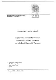
5.3 ime interaion process 

Picture 1 shows the whole process of he time integration method. The program 

comes to an end when the final time or the maximal step number are 

eached or when the maximal number of sep ize reducions wihin one negraton 

ep is exceeded.

espping 

5.4 Grid managent 

The program KASKADE supports work with several grids which are connected 

to a list. A time integration requires to exchange values on differently 

efined grids. This leads to cos eek algorihms. To be more efective here, 

he srucure EDG is enlarged he new elent 

*twin 

If the considered edge exists in he other triangulation, then this elemen 

points at he corresponding element, otherwise it is nil. In the structur 

TRIANGULATION the new element int twinRelation stands for the e 

istence of such a relation between two triangulations. 

To work wih tw grids the folowing funcons can be used: 

int SetTwinRelOnCoarseGrids(TRIANGULATI *t,RIUL *t) 

inializes the twirelaton of two arse grids. 

DG *FindBrotherEdge(real ,EDG *edFrom 

nds the edge of the other grid n which a given poin ies. 

real InterpolateInEdge(real E *edn,int var,int inde 

gives back an nterpolated value. 

17

haper 

le 

In this chapte how how to add a new problem to the list of predefined 

problems: 

define a s of functions to characerize the inial boundary value probem 

add the problem to the list of predefined problems (call etProblem, 

using nitUserTime in user. of the kardos-directory, 

add tw ommon car grids in the grids-directory, 

use kardos . startup for an automatic ommand language dialog wi 

the sysem 

6.1 ser functions for opulation ecolo del 

Let us olve the folowing equatons 

- 0. 

+ 1-u 

in the domain 0 ) for t > 0, with the boundary condons 

and the initial condition 

= 0 for t > x = 0 and x = 

5 for 

4x + 1 for 

-4x + 11 for 

for 

10 for 

4x + for 

-4x + for 

for 

18

This system of nonlinear equations modls a cerain planktonit predator 

prey suations in which crowding is a facor. The KARDOS user defines in 

user. he following funtions: 

static int EcoParabolic(real x, int classA, real t, real *fVals, 

int equation, int variable) 

if (equation!=variable) return F_IGN0RE; 

switch (variable) 

{ 

case 0: fVals[0] = 1.0; 

break; 

case 1: fVals[0] = 1.0; 

break; 

return F_C0ISTAIT; 

static int EcoLaplace(real x, int classA, real t, real *fVals, 


if (equation!=variable) return F_IGN0RE; 


{ case 0: fVals[0] = 0.0125; 

break; 

case 1: fVals[0] = 1.0; 

break; 

return F_C0ISTAIT; 

static int EcoConvection(real x, int classA, real t, real *fVal, 


return F_IGI0RE; 

static int EcoHelmholtz(real x, int classA, real t, real *fVal, 


return F_IGI0RE; 

static int EcoSource(real x, int classA, real t, EDG* ed,

eal valO, vail; 

real *fVal, int equation, 

real (*Func)(real,EDG*,int,timeIntegMethod*)) 

switch (equation) 

{ 

case 0: valO = Func(x,ed,0,actTimeIntegtor); 

vail = Func(x,ed,l,actTimeIntegtor); 

fVal[0] = ((35.0+16.0*val0-val0*val0)/9.0-vall)*val0; 

break; 

case 1: valO = Func(x,ed,0,actTimeIntegtor); 


fVal[0] = (val0-1.0-0.4*vall)*vall; 

break; 

return F_VARIABLE; 

static int EcoJacobian(real x, int classA, real t, EDG* ed, real *fVal, 

int equation, int variable, 

real (*Func)(real,EDG*,int,timeIntegMethod*)) 

real valO, vail; 

switch (equation) 

{ 

case 0: if (variable==0) 

{ 

valO = Func(x,ed,0,actTimeIntegtor); 


fVal[0] = (35.0+32.0*val0-3.0*val0*val0)/9.0-vall; 

else if (variable==l) 

{ 


fVal[0] = -vail; 

else ZIBStdOut("error in EcoJacobian\n"); 

break; 

case 1: if (variable==0) 

{ 


fVal[0] = vail;

eturn F_VARIABLE; 

else if (variable==l) 

{ 

valO = Func(x,ed,0,actTimeIntegtor); 


fVal[0] = val0-1.0-0.*vall; 

else ZIBStdOut("error in EcoJacobian\n"); 

break; 

static real EcoInitialFunc(real x, int classA, int variable) 

{ 

real val = 0.0; 


{ 

case 0: if ((0.0

fVals[l] = 0.0; /* */ 

else ZIBStdOutCerror in EcoCauchy\n"); 

break; 

case 1: i ((x==0.0)I I(x==2.5)) 

fVals[0] =0.0; /* Sigma */ 

fVals[l] = 0.0; /* i */ 

return F_COISTAIT; 

eise ZIBStdOutC"error in EcoCauchy\n"); 

break; 

6.2 Defining the new problem 

ext we defne the new problem wih the help of the following procedure 

int InitUserTimeQ 

{ 

f (!SetTimeProblem("example1",varName, 

EcoParabolic, 

EcoLaplace, 

EcoConvection, 

EcoHelmholtz, 

EcoSource, 

EcoJacobian, 

EcoInitialFunc, 

EcoCauchy, 

EcoDirichlet, 

(int(*)(real,int,real,real*,int))nil)); 

return true; 

A call of nitTimeUser is carried out automatically from he main program 

6.3 roviding tw como coar rid 

Now we inser two arse grids n the grids-decory using the files ecologyl 

and cology2 

ecologyl ecology2 

Dimension:(11,10) Dimension:(11,0) 

22

0 0.0,B,CC 0 0.0,B,CC 

1:0.25,1,11 1:0.25,1,11 

2:0.5,1,11 2:0.5,1,11 

3:0.5,1,11 3:0.5,1,11 

4:1.0,1,11 4:1.0,1,11 

5:1.25,1,11 5:1.25,1,11 

6:1.5,1,11 6:1.5,1,11 

:1.5,1,11 1.5,1,11 

:2.0,1,11 :2.0,1,11 

9:2.25,1,11 9:2.25,1,11 

0:2.5,B,CC 10:2.5,B,CC 

EID EID 

0 (0,1) 0 (0,1) 

1 (1,2) 1 (1,2) 

2 (2,3) 2 (2,3) 

3 (3,4) 3 (3,4) 

4 (4,5) 4 (4,5) 

5 (5,6) 5 (5,6) 

6 (6, 6 (6, 

( ( 

(9) (9) 

9 (9,0) 9 (9,10) 

EID EID 

6.4 ialo with the ste 

KARDOS reads at the tart a file kardos.startup which contains a sequenc 

of commands and executes these commands. That way we get an automat 

dialog wih the system. Of course, a step-by-step ialog is available to. 

deposit in kardos.starup the following omands: 

read ../grids/ecologyl.g 

read ../grids/ecology2.g 

timeproblem examplel 

seliterate pbicgstabtime 

selmatmul sparse 

selestimate babuska 

selrefine meanval 

seltimeinteg rodas 

window new automatic name solutionl 

graphic solution triangulation 

seldraw 0 

window new automatic name solution2 

graphic solution triangulation

seldraw 1 

timesteppin timestep 0.0001 maxsteps 200 globTol 0.02 tEnd 10.0 

ow we can start the program

ferences 

Babus, W.C. Rheinboldt: Error estimas for adptive fin et 

comutons. SIAM J. Numer. Anal 15 p. 7364 (1978) 

] P. Deuflhard, P. Leinen, H. Yserentant: Concepts an Adaptie Herarcal 

F e Elen Code. IMPACT, , p. 3-3 1989) 

3] B. Erdmann, J. Lang, R. Roitzsch: KASKADE - Manual. To appear as 

Technical Report TR 93-5, Konrad-Zus-Zentrum (ZIB) (1993) 

[4] J. Lang, A. Walter: A Fnie Eent Method Adaptive n Space and 

Tim for Nonlinear Reaction-Dffuson Systems. IMPAC of Comput 

ing Scence and Engineerng, , p. 9-314 (199 

] J. Lang, A Walter: An Adaptive Rothe Method for Nonlinear Reacon- 

Diffuson Sstms. Appled Numerial Mathematics 13 p. 1 1 4 

1993) 

M. Roche: Rosenbrock Methods for ifferenal Albraic Equatons. 

umer Math. 52, p. 4 (1 

Acknowledgements. I acknowledge R. Roitzsch for inspiring disussions 

on the field of programming and for making available always he urrent 

version of KASKADE. I also thank U. Nowak for supplying me wih referen 

olutions obtained y his finite dfferene method.

skade eaction ffusion ne-dimensional System - ZIB

You also want an ePaper? Increase the reach of your titles

Delete template?

Save as template?