PDF-6.4MB - Faculty of Industrial Engineering and Management

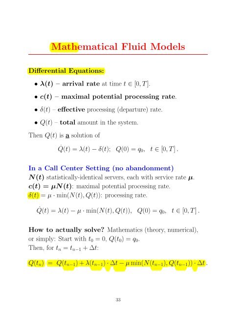
Mathematical Fluid Models
Differential Equations:
• λ(t) – arrival rate at time t ∈ [0, T ].
• c(t) – maximal potential processing rate.
• δ(t) – effective processing (departure) rate.
• Q(t) – total amount in the system.
Then Q(t) is a solution of
˙Q(t) = λ(t) − δ(t); Q(0) = q0, t ∈ [0, T ] .
In a Call Center Setting (no abandonment)
N(t) statistically-identical servers, each with service rate µ.
c(t) = µN(t): maximal potential processing rate.
δ(t) = µ · min(N(t), Q(t)): processing rate.
˙Q(t) = λ(t) − µ · min(N(t), Q(t)), Q(0) = q0, t ∈ [0, T ] .
How to actually solve? Mathematics (theory, numerical),
or simply: Start with t0 = 0, Q(t0) = q0.
Then, for tn = tn−1 + ∆t:
Q(tn) = Q(tn−1) + λ(tn−1) · ∆t − µ min(N(tn−1), Q(tn−1)) · ∆t .
33