PDF-6.4MB - Faculty of Industrial Engineering and Management
PDF-6.4MB - Faculty of Industrial Engineering and Management
PDF-6.4MB - Faculty of Industrial Engineering and Management

Create successful ePaper yourself
Turn your PDF publications into a flip-book with our unique Google optimized e-Paper software.
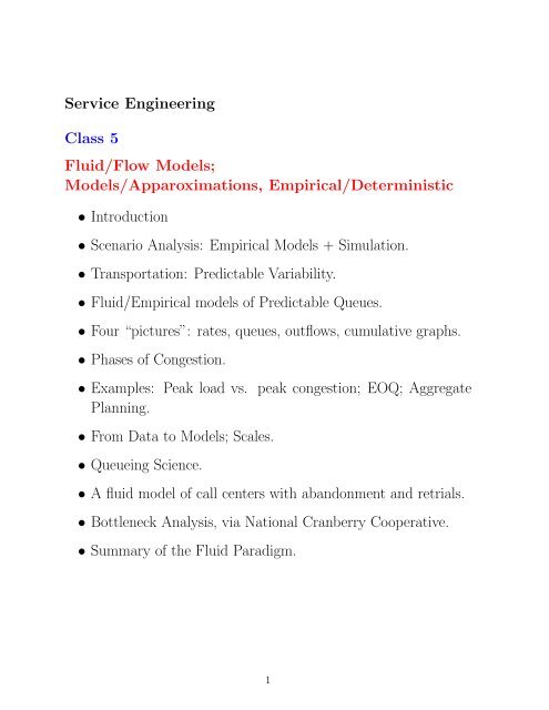
Service <strong>Engineering</strong><br />
Class 5<br />
Fluid/Flow Models;<br />
Models/Apparoximations, Empirical/Deterministic<br />
• Introduction<br />
• Scenario Analysis: Empirical Models + Simulation.<br />
• Transportation: Predictable Variability.<br />
• Fluid/Empirical models <strong>of</strong> Predictable Queues.<br />
• Four “pictures”: rates, queues, outflows, cumulative graphs.<br />
• Phases <strong>of</strong> Congestion.<br />
• Examples: Peak load vs. peak congestion; EOQ; Aggregate<br />
Planning.<br />
• From Data to Models; Scales.<br />
• Queueing Science.<br />
• A fluid model <strong>of</strong> call centers with ab<strong>and</strong>onment <strong>and</strong> retrials.<br />
• Bottleneck Analysis, via National Cranberry Cooperative.<br />
• Summary <strong>of</strong> the Fluid Paradigm.<br />
1
Keywords: Blackboard Lecture<br />
• Classes 1-4 = Introduction to Introduction:<br />
On Services, Measurements, Models: Empirical, Stochastic.<br />
Today, our first model <strong>of</strong> a Service Stations: Fluid Models.<br />
• Fluid Model vs. Approximation<br />
• Model: Fluid/Flow, Deterministic/Empirical; eg. EOQ.<br />
• Conceptualize: busy highway around a large airport at night.<br />
• Types <strong>of</strong> queues: Perpetural, Predictable, Stochastic.<br />
• On Variability: Predictable vs. Stochastic (Natural/Artificial).<br />
• Scenario Analysis vs. Averaging, Steady-State.<br />
• Descriptive Model (Inside the Black Box), via 4 “pictures”:<br />
rates, queues, outflows, cummulants.<br />
• Mathematical Model (Black Box), via differential equations.<br />
• Resolution/Units (Scales).<br />
• Applications:<br />
– Phenomena:<br />
Peaks (load vs. congestion); Calmness after a storm;<br />
– Managerial Support:<br />
Staffing (Recitation); Bottlenecks (Cranberries)<br />
• Bottlenecks.<br />
2
Types <strong>of</strong> Queues<br />
• Perpetual Queues: every customers waits.<br />
– Examples: public services (courts), field-services, operating<br />
rooms, . . .<br />
– How to cope: reduce arrival (rates), increase service capacity,<br />
reservations (if feasible), . . .<br />
– Models: fluid models.<br />
• Predictable Queues: arrival rate exceeds service capacity<br />
during predictable time-periods.<br />
– Examples: Traffic jams, restaurants during peak hours,<br />
accountants at year’s end, popular concerts, airports (security<br />
checks, check-in, customs) . . .<br />
– How to cope: capacity (staffing) allocation, overlapping<br />
shifts during peak hours, flexible working hours, . . .<br />
– Models: fluid models, stochastic models.<br />
• Stochastic Queues: number-arrivals exceeds servers’ capacity<br />
during stochastic (r<strong>and</strong>om) periods.<br />
– Examples: supermarkets, telephone services, bank-branches,<br />
emergency-departments, . . .<br />
– How to cope: dynamic staffing, information (e.g. reallocate<br />
servers), st<strong>and</strong>ardization (reducing std.: in arrivals,<br />
via reservations; in services, via TQM) ,. . .<br />
– Models: stochastic queueing models.<br />
3
Economist.com<br />
Crowded airports<br />
L<strong>and</strong>ing flap<br />
Apr 4th 2007<br />
From The Economist print edition<br />
A tussle over Heathrow threatens a longst<strong>and</strong>ing monopoly<br />
TO DEATH <strong>and</strong> taxes, one can now add jostling queues <strong>of</strong> frustrated travellers at<br />
Heathrow as one <strong>of</strong> life's unhappy certainties. Stephen Nelson, the chief executive <strong>of</strong><br />
BAA, which owns the airport, does little to inspire confidence that those passing<br />
through his domain this Easter weekend will avoid the fate <strong>of</strong> the thous<strong>and</strong>s str<strong>and</strong>ed<br />
in tents by fog before Christmas or trapped in twisting lines by a security scare in the<br />
summer. In the Financial Times on April 2nd he wrote <strong>of</strong> the difficulties <strong>of</strong> managing<br />
“huge passenger dem<strong>and</strong> on our creaking transport infrastructure”, <strong>and</strong> gave warning<br />
that “the elements can upset the best laid plans”.<br />
Blaming the heavens for chaos that has yet to ensue may be good public relations but<br />
Mr Nelson's real worries have a more earthly origin. On March 30th two regulators<br />
released reports on his firm, one threatening to cut its pr<strong>of</strong>its <strong>and</strong> the other to break it<br />
up. First the Civil Aviation Authority (CAA), which oversees airport fees, said it was<br />
thinking <strong>of</strong> reducing the returns that BAA is allowed to earn from Heathrow <strong>and</strong><br />
Gatwick airports. Separately the Office <strong>of</strong> Fair Trading (OFT) asked the Competition<br />
Commission to investigate BAA's market dominance. As well as Heathrow, Europe's<br />
main gateway on the transatlantic air route, BAA owns its two principal London<br />
competitors, Gatwick <strong>and</strong> Stansted, <strong>and</strong> several other airports.<br />
http://www.economist.com/world/britain/PrinterFriendly.cfm?story_id=8966398 (1 <strong>of</strong> 3)4/9/2007 5:30:10 PM<br />
Rex
The “Fluid View”<br />
or Flow Models <strong>of</strong> Service Networks<br />
Service <strong>Engineering</strong> (Science, <strong>Management</strong>)<br />
December, 2006<br />
1 Predictable Variability in Time-Varying Services<br />
Time-varying dem<strong>and</strong> <strong>and</strong> time-varying capacity are common-place in service operations. Sometimes,<br />
predictable variability (eg. peak dem<strong>and</strong> <strong>of</strong> about 1250 calls on Mondays between 10:00-<br />
10:30, on a regular basis) dominates stochastic variability (i.e. r<strong>and</strong>om fluctuations around the<br />
1250 dem<strong>and</strong> level). In such cases, it is useful to model the service system as a deterministic fluid<br />
model, which transportation engineers st<strong>and</strong>ardly practice. We shall study such fluid models, which<br />
will provide us with our first mathematical model <strong>of</strong> a service-station.<br />
A common practice in many service operations, notably call centers <strong>and</strong> hospitals, is to timevary<br />
staffing in response to time-varying dem<strong>and</strong>. We shall be using fluid-models to help determine<br />
time-varying staffing levels that adhere to some pre-determined criterion. One such criterion is<br />
“minimize costs <strong>of</strong> staffing plus the cost <strong>of</strong> poor service-quality”, as will be described in our fluidclasses.<br />
Another criterion, which is more subtle, strives for time-stable performance in the face <strong>of</strong> timevarying<br />
dem<strong>and</strong>. We shall accommodate this criterion in the future (in the context <strong>of</strong> what will<br />
be called “the square-root rule” for staffing). For now, let me just say that the analysis <strong>of</strong> this<br />
criterion helped me also underst<strong>and</strong> a phenomenon that has frustrated me over many years, which<br />
I summarize as “The Right Answer for the Wrong Reasons”, namely: how come so many call<br />
centers enjoy a rather acceptable <strong>and</strong> <strong>of</strong>ten good performance, despite the fact that their managers<br />
noticeably lack any “stochastic” underst<strong>and</strong>ing (in other words, they are using a “Fluid-View” <strong>of</strong><br />
their systems).<br />
2 Fluid/Flow Models <strong>of</strong> Service Networks<br />
We have discussed why it is natural to view a service network as a queueing network. Prevalent<br />
models <strong>of</strong> the latter are stochastic (r<strong>and</strong>om), in that they acknowledge uncertainty as being a central<br />
characteristic. It turned out, however, that viewing a queueing network through a “deterministic<br />
eye”, animating it as a fluid network, is <strong>of</strong>ten appropriate <strong>and</strong> useful. For example, the Fluid View<br />
<strong>of</strong>ten suffices for bottleneck (capacity) analysis (the “Can we do it?” step, which is the first step<br />
in analyzing a dynamic stochastic network); for motivating congestion laws (eg. Little’s Law, or<br />
”Why peak congestion lags behind peak load”); <strong>and</strong> for devising (first-cut) staffing levels (which<br />
are sometime last-cut as well).<br />
1
Some illuminating “Fluid” quotes:<br />
• ”Reducing letter delays in post-<strong>of</strong>fices”: ”Variation in mail flow are not so much due to r<strong>and</strong>om<br />
fluctuations about a known mean as they are time-variations in the mean itself . . . Major contributor<br />
to letter delay within a post<strong>of</strong>fice is the shape <strong>of</strong> the input flow rate: about 70% <strong>of</strong> all<br />
letter mail enters a post <strong>of</strong>fice within 4-hour period”. (From Oliver <strong>and</strong> Samuel, a classical 1962<br />
OR paper).<br />
• ” . . . a busy freeway toll plaza may have 8000 arrivals per hour, which would provide a coefficient<br />
<strong>of</strong> variation <strong>of</strong> just 0.011 for 1 hour. This means that a non-stationary Poisson arrivals pattern<br />
can be accurately approximated with a deterministic model”. (Hall’s textbook, pages 187-8).<br />
Note: the statement is based on a Poisson model, in which mean = variance.<br />
There is a rich body <strong>of</strong> literature on Fluid Models. It originates in many sources, it takes many<br />
forms, <strong>and</strong> it is powerful when used properly. For example, the classical EOQ model takes a fluid<br />
view <strong>of</strong> an inventory system, <strong>and</strong> physicists have been analyzing macroscopic models for decades.<br />
Not surprisingly, however, the first explicit <strong>and</strong> influential advocate <strong>of</strong> the Fluid View to queueing<br />
systems is a Transportation Engineer (Gordon Newell, mentioned previously). To underst<strong>and</strong> why<br />
this view was natural to Newell, just envision an airplane that is l<strong>and</strong>ing in an airport <strong>of</strong> a large<br />
city, at night - the view, in rush-hour, <strong>of</strong> the network <strong>of</strong> highways that surrounds the airport, as<br />
seen from the airplane, is precisely this fluid-view. (The influence <strong>of</strong> Newel1 is clear in Hall’s book.)<br />
Some main advantages <strong>of</strong> fluid-models, as I perceive them, are:<br />
• They are simple (intuitive) to formulate, fit (empirically) <strong>and</strong> analyze (elementary). (See the<br />
Homework on Empirical Models.)<br />
• They cover a broad spectrum <strong>of</strong> features, relatively effortlessly.<br />
• Often, they are all that is needed, for example in analyzing capacity, bottlenecks or utilization<br />
pr<strong>of</strong>iles (as in National Cranberries Cooperative <strong>and</strong> HW2).<br />
• They provide useful approximations that support both performance analysis <strong>and</strong> control. (The<br />
approximations are formalized as first-order deterministic fluid limits, via Functional (Strong)<br />
Laws <strong>of</strong> Large Numbers.)<br />
Fluid models are intimately related to Empirical Models, which are created directly from measurements.<br />
As such, they constitute a natural first step in modeling a service network. Indeed,<br />
refining a fluid model <strong>of</strong> a service-station with the outcomes <strong>of</strong> Work (Time <strong>and</strong> Motion) Studies<br />
(classical <strong>Industrial</strong> <strong>Engineering</strong>), captured in terms <strong>of</strong> say histograms, gives rise to a (stochastic)<br />
model <strong>of</strong> that service station.<br />
2
Contents<br />
• Scenario Analysis: Empirical Models + Simulation.<br />
• Transportation: Predictable Variability.<br />
• Fluid/Empirical models <strong>of</strong> Predictable Queues.<br />
• Four “pictures”: rates, queues, outflows, cumulative<br />
graphs.<br />
• Phases <strong>of</strong> Congestion.<br />
• Examples: Peak load vs. peak congestion; EOQ;<br />
Aggregate Planning.<br />
• From Data to Models; Scales.<br />
• Queueing Science.<br />
• A fluid model <strong>of</strong> call centers with ab<strong>and</strong>onment <strong>and</strong><br />
retrials.<br />
• Bottleneck Analysis, via National Cranberry Cooperative.<br />
• Summary <strong>of</strong> the Fluid Paradigm.<br />
2
Labor-Day Queueing in Niagara Falls<br />
Three-station T<strong>and</strong>em Network:<br />
Elevators, Coats, Boats<br />
Conceptual Fluid Model<br />
Total wait <strong>of</strong> 15 minutes<br />
from upper-right corner to boat<br />
Customers/units are modeled by fluid (continuous) flow.<br />
How? “Deterministic” constant motion<br />
Labor-day Queueing at Niagara Falls<br />
• Appropriate when predictable variability prevalent;<br />
• Useful first-order models/approximations, <strong>of</strong>ten suffice;<br />
• Rigorously justifiable via Functional Strong Laws <strong>of</strong> Large<br />
Numbers.<br />
30
Shouldice Hospital: Flow Chart <strong>of</strong> Patients’ Experience<br />
Day 1:<br />
Waiting<br />
Room<br />
1:00-3:00 PM<br />
Day 2:<br />
Pre Op<br />
Room<br />
5:30-7:30 AM<br />
to 3:00 PM<br />
Day 3:<br />
Day 4:<br />
Patient’s<br />
Room<br />
6:00 AM<br />
Dining<br />
Room<br />
7:45-8:50 AM<br />
Surgeons Admit<br />
Exam Room<br />
(6)<br />
15-20 min<br />
Orient’n<br />
Room<br />
5:00-5:30 PM<br />
Operating<br />
Room<br />
45 min<br />
60-90 min<br />
Dining Room<br />
7:45-8:15 AM<br />
Remove<br />
Rem. Clips<br />
Clinic<br />
Acctg.<br />
Office<br />
10 min<br />
Dining<br />
Room<br />
5:30-6:00 PM<br />
Post Op<br />
Room<br />
Remove Clips<br />
Clinic<br />
Room?<br />
Stay Longer<br />
Go Home<br />
Nurses’<br />
Station<br />
5-10 min<br />
Rec Lounge<br />
7:00-9:00 PM<br />
Patient’s<br />
Room<br />
Rec Room<br />
Grounds<br />
Dining<br />
Room<br />
9:00 PM<br />
Dining<br />
Room<br />
9:00 PM<br />
•External types <strong>of</strong> abdominal hernias.<br />
•82% 1 st -time repair.<br />
•18% recurrences.<br />
•6850 operations in 1986.<br />
•Recurrence rate: 0.8% vs. 10%<br />
Industry Std.<br />
Patient’s<br />
Room<br />
1-2 hours<br />
Patient’s<br />
Room<br />
9:30 PM-<br />
5:30 AM
31<br />
Queue<br />
Empirical Fluid Model: Queue-Length at a Bank Queue<br />
Catastrophic/Heavy/Regular Day(s)<br />
60<br />
50<br />
40<br />
30<br />
20<br />
10<br />
Bank Queue<br />
0<br />
8 8.5 9 9.5 10 10.5 11 11.5 12 12.5 13<br />
Time <strong>of</strong> Day<br />
Catastrophic Heavy Load Regular
Daily Queues<br />
Israeli Call Center, November 1999<br />
number <strong>of</strong> calls<br />
number <strong>of</strong> calls<br />
number <strong>of</strong> calls<br />
14<br />
12<br />
10<br />
14<br />
12<br />
10<br />
8<br />
6<br />
4<br />
2<br />
0<br />
14<br />
12<br />
10<br />
8<br />
6<br />
4<br />
2<br />
0<br />
8<br />
6<br />
4<br />
2<br />
0<br />
07:00<br />
08:00<br />
09:00<br />
10:00<br />
11:00<br />
12:00<br />
13:00<br />
14:00<br />
15:00<br />
07:00<br />
08:00<br />
09:00<br />
10:00<br />
11:00<br />
12:00<br />
13:00<br />
14:00<br />
15:00<br />
07:00<br />
08:00<br />
09:00<br />
10:00<br />
11:00<br />
12:00<br />
13:00<br />
14:00<br />
15:00<br />
20<br />
16:00<br />
time<br />
16:00<br />
time<br />
16:00<br />
time<br />
queue<br />
queue<br />
queue<br />
17:00<br />
18:00<br />
19:00<br />
20:00<br />
21:00<br />
22:00<br />
23:00<br />
00:00<br />
17:00<br />
18:00<br />
19:00<br />
20:00<br />
21:00<br />
22:00<br />
23:00<br />
00:00<br />
17:00<br />
18:00<br />
19:00<br />
20:00<br />
21:00<br />
22:00<br />
23:00<br />
00:00
Average Monthly Queues<br />
Israeli Call Center, November 1999<br />
Average number in queue<br />
Average number in queue<br />
5<br />
4.5<br />
4<br />
3.5<br />
3<br />
2.5<br />
2<br />
1.5<br />
1<br />
0.5<br />
1<br />
0.9<br />
0.8<br />
0.7<br />
0.6<br />
0.5<br />
0.4<br />
0.3<br />
0.2<br />
0.1<br />
0<br />
0<br />
Time<br />
all PS<br />
07:00<br />
08:00<br />
09:00<br />
10:00<br />
11:00<br />
12:00<br />
13:00<br />
14:00<br />
15:00<br />
16:00<br />
17:00<br />
18:00<br />
19:00<br />
07:00<br />
20:00<br />
08:00<br />
21:00<br />
09:00<br />
22:00<br />
10:00<br />
23:00<br />
11:00<br />
12:00<br />
13:00<br />
14:00<br />
15:00<br />
16:00<br />
17:00<br />
18:00<br />
19:00<br />
20:00<br />
21:00<br />
22:00<br />
23:00<br />
19<br />
Time<br />
IN NE NW
Number <strong>of</strong> cases<br />
9000<br />
8000<br />
7000<br />
6000<br />
5000<br />
4000<br />
3000<br />
2000<br />
1000<br />
Arrivals to queue<br />
September 2001<br />
0<br />
00:00 02:00 04:00 06:00 08:00 10:00 12:00 14:00 16:00 18:00 20:00 22:00<br />
Time (Resolution 60 min.)<br />
04.09.2001 11.09.2001 18.09.2001 25.09.2001
Number <strong>of</strong> cases<br />
120<br />
100<br />
80<br />
60<br />
40<br />
20<br />
Arrivals to queue<br />
September 2001<br />
0<br />
00:00 02:00 04:00 06:00 08:00 10:00 12:00 14:00 16:00 18:00 20:00 22:00<br />
Time (Resolution 30 sec.)<br />
04.09.2001 11.09.2001 18.09.2001 25.09.2001
Optimizing Patient Flow by Managing Its Variability C H A P T E R 4<br />
FIGURE 4.1<br />
Tracking Patient Census<br />
This graph represents typical hospital census for weekdays (each point represents a<br />
day). The peaks <strong>and</strong> valleys represent residuals from the mean census identified by<br />
the dashed line.<br />
decision to discharge a patient from the ED or maybe to transfer a patient when,<br />
under normal circumstances, the patient would be admitted.Thus, a hospital<br />
underutilizes its resources on one day, <strong>and</strong> the next day these resources are put<br />
under stress with resultant consequences for access to <strong>and</strong> quality <strong>of</strong> care.<br />
One may conclude that hospital capacity in its current form is not sufficient<br />
to guarantee quality care. Does the health care delivery system need additional<br />
resources? The typical answer is “yes.”Then, the next logical question is What<br />
additional resources are needed to guarantee quality care? For example,What kind<br />
<strong>of</strong> beds does a particular hospital need? Does it need more ICU beds? more<br />
maternity beds? more telemetry beds? If yes, how many?<br />
Surprisingly, not many hospitals, if any, can justify their answers to those questions.<br />
They cannot specifically demonstrate how many <strong>of</strong> which types <strong>of</strong> beds will<br />
guarantee quality <strong>of</strong> care. But consider an individual going to the bank under<br />
similar circumstances to borrow money. In response, the bank, asks two basic<br />
97
Predicting Emergency Department Status<br />
Houyuan Jiang‡, Lam Phuong Lam†, Bowie Owens†, David Sier† <strong>and</strong> Mark Westcott†<br />
† CSIRO Mathematical <strong>and</strong> Information Sciences, Private Bag 10,<br />
South Clayton MDC, Victoria 3169, Australia<br />
‡ The Judge Institute <strong>of</strong> <strong>Management</strong>, University <strong>of</strong> Cambridge,<br />
Trumpington Street, Cambridge CB2 1AG, UK<br />
Abstract<br />
Many acute hospitals in Australia experience frequent episodes <strong>of</strong> ambulance bypass.<br />
An important part <strong>of</strong> managing bypass is the ability to determine the likelihood <strong>of</strong> it<br />
occurring in the near future.<br />
We describe the implementation <strong>of</strong> a computer program designed to forecast the<br />
likelihood <strong>of</strong> bypass. The forecasting system is designed to be used in an Emergency<br />
Department. In such an operational environment, the focus <strong>of</strong> the clinicians is on<br />
treating patients, there is no time carry out any analysis <strong>of</strong> the historical data to be used<br />
for forecasting, or to determine <strong>and</strong> apply an appropriate smoothing method.<br />
The method is designed to automate the short term prediction <strong>of</strong> patient arrivals. It<br />
uses a multi-stage data aggregation scheme to deal with problems that may arise from<br />
limited arrival observations, an analysis phase to determine the existence <strong>of</strong> trends <strong>and</strong><br />
seasonality, <strong>and</strong> an optimisation phase to determine the most appropriate smoothing<br />
method <strong>and</strong> the optimal parameters for this method.<br />
The arrival forecasts for future time periods are used in conjunction with a simple<br />
dem<strong>and</strong> modelling method based on a revised stationary independent period by period<br />
approximation queueing algorithm to determine the staff levels needed to service the<br />
likely arrivals <strong>and</strong> then determines a probability <strong>of</strong> bypass based on a comparison <strong>of</strong><br />
required <strong>and</strong> available resources.<br />
1 Introduction<br />
This paper describes a system designed to be part <strong>of</strong> the process for managing Emergency Department<br />
(ED) bypass. An ED is on bypass when it has to turn away ambulances, typically because all<br />
cubicles are full <strong>and</strong> there is no opportunity to move patients to other beds in the hospital, or because<br />
the clinicians on duty are fully occupied dealing with critical patients who require individual care.<br />
Bypass management is part <strong>of</strong> the more general bed management <strong>and</strong> admission–discharge<br />
procedures in a hospital. However, a very important part <strong>of</strong> determining the likelihood <strong>of</strong> bypass<br />
occurring in the near future, typically the next 1, 4 or 8 hours, is the ability to predict the probable<br />
patient arrivals, <strong>and</strong> then, given the current workload <strong>and</strong> staff levels, the probability that there will<br />
be sufficient resources to deal with these arrivals.<br />
Here, we consider the implementation <strong>of</strong> a multi-stage forecasting method [1] to predict patient<br />
arrivals, <strong>and</strong> a dem<strong>and</strong> management queueing method [2], to assess the likelihood <strong>of</strong> ED bypass.<br />
The prototype computer program implementing the method has been designed to run on a hospital<br />
intranet <strong>and</strong> to extract patient arrival data from hospital patient admission <strong>and</strong> ED databases.<br />
The program incorporates a range <strong>of</strong> exponential smoothing procedures. A user can specify the<br />
particular smoothing procedure for a data set or to configure the program to automatically determine<br />
the best procedure from those available <strong>and</strong> then use that method.<br />
For the results presented here, we configured the program to automatically find the best smoothing<br />
method since this is the way it is likely to be used in an ED where the staff are more concerned<br />
with treating patients than configuring forecast smoothing parameters.
Patients per Hour<br />
Average Patients per Hour<br />
Average Patients per Hour<br />
16<br />
14<br />
12<br />
10<br />
8<br />
6<br />
4<br />
2<br />
0<br />
1/7/2002<br />
10<br />
9<br />
8<br />
7<br />
6<br />
5<br />
4<br />
3<br />
2<br />
1<br />
2/7/2002<br />
Monday<br />
Tuesday<br />
Wednesday<br />
Thursday<br />
Friday<br />
Saturday<br />
Sunday<br />
3/7/2002<br />
4/7/2002<br />
5/7/2002<br />
(a) Week beginning July 1, 2002<br />
6/7/2002<br />
7/7/2002<br />
8/7/2002<br />
Arrivals averaged over 60 weeks from Mon 4/06/2001 to Sun 28/07/2002<br />
0<br />
1 2 3 4 5 6 7 8 9 10 11 12 13 14 15 16 17 18 19 20 21 22 23 24<br />
16<br />
14<br />
12<br />
10<br />
8<br />
6<br />
4<br />
2<br />
0<br />
Monday<br />
Tuesday<br />
Wednesday<br />
(b) Average by day <strong>of</strong> week<br />
Arrivals averaged over 60 weeks from Mon 4/06/2001 to Sun 28/07/2002<br />
Thursday<br />
Friday<br />
(c) Average weekly<br />
Saturday<br />
Figure 1: Hourly patient arrivals, June 2001 to July 2002<br />
Sunday<br />
For the optimisation we assume no a priori knowledge <strong>of</strong> the patient arrival patterns. The process<br />
involves simply fitting each <strong>of</strong> the nine different methods listed in Table 1 to the data, using the mean<br />
square fitting error, calculated using (3), as the objective function. The smoothing parameters for<br />
each method are all in (0, 1) <strong>and</strong> the parameter solution space is defined by a set <strong>of</strong> values obtained<br />
from an appropriately fine uniform discretization <strong>of</strong> this interval. The optimal values for each<br />
method are then obtained from a search <strong>of</strong> all possible combinations <strong>of</strong> the parameter values.
From the data aggregated at a daily level, repeat the procedure to extract data for each<br />
hour <strong>of</strong> the day to form 24 time series (12am–1am, 1am–2am, ..., 11pm–12am). Apply the<br />
selected smoothing method, or the optimisation algorithm, to each time series <strong>and</strong> generate<br />
forecasting data for those future times <strong>of</strong> day within the requested forecast horizon. The<br />
forecast data generated for each time <strong>of</strong> day are scaled uniformly in each day in order to<br />
match the forecasts generated from the previously scaled daily data.<br />
Output: Display the historical <strong>and</strong> forecasted data for each <strong>of</strong> the sets <strong>of</strong> aggregated observations<br />
constructed during the initialisation phase.<br />
The generalisation <strong>of</strong> these stages is straightforward. For example, if the data was aggregated to a<br />
four-weekly (monthly) level, then the first scaling step would be to extract the observations from<br />
the weekly data to form four time series, corresponding to the first, second, third <strong>and</strong> fourth week<br />
<strong>of</strong> each month. Historical data at timescales <strong>of</strong> less than one day are scaled to the daily forecasts.<br />
For example, observations at a half-hourly timescale are used to form 48 time series for scaling to<br />
the day forecasts.<br />
4.3 Output from the multi-stage method<br />
Figures 2 <strong>and</strong> 3 show some <strong>of</strong> the results obtained from using the multi-stage forecasting method to<br />
predict ED arrivals using the 60 weeks <strong>of</strong> patient arrival data described in Section3. The forecasted<br />
data were generated from an optimisation that used the multi-stage forecasting method to minimise<br />
the residuals <strong>of</strong> (3) across all the smoothing methods in Table 1.<br />
Patients per Hour<br />
Patients per 4 Hours<br />
22<br />
20<br />
18<br />
16<br />
14<br />
12<br />
10<br />
8<br />
6<br />
4<br />
2<br />
0<br />
25/07/2002<br />
60<br />
55<br />
50<br />
45<br />
40<br />
35<br />
30<br />
25<br />
20<br />
15<br />
10<br />
5<br />
0<br />
25/07/2002<br />
26/07/2002<br />
27/07/2002<br />
Historical data: Mon 4/06/2001 to Sun 28/07/2002, 420 days<br />
28/07/2002<br />
29/07/2002<br />
Historical<br />
Forecasted<br />
30/07/2002<br />
Figure 2: Hourly historical <strong>and</strong> forecasted data 25/7/2002–31/7/2002<br />
26/07/2002<br />
27/07/2002<br />
28/07/2002<br />
29/07/2002<br />
30/07/2002<br />
31/07/2002<br />
Historical data: Mon 4/06/2001 to Sun 28/07/2002, 420 days<br />
Historical<br />
Forecasted<br />
Figure 3: Four-hourly historical <strong>and</strong> forecasted data 25/7/2002–31/7/2002<br />
31/07/2002
Optimizing Patient Flow by Managing Its Variability C H A P T E R 4<br />
Identifying Paths <strong>of</strong> Patient Flow in the Hospital<br />
Emergency<br />
Department<br />
FIGURE 4.3<br />
Intensive Care<br />
Unit<br />
Medical/Surgical<br />
Floors<br />
This diagram represents patient flow within a hospital. Natural <strong>and</strong> artificial variability<br />
are represented by emergency department admissions <strong>and</strong> scheduled dem<strong>and</strong>.<br />
ED overcrowding is so pervasive that sometimes we have the attitude that it<br />
affects everyone the same way. But according to Brad Prenney, deputy director<br />
<strong>of</strong> Boston University’s Program for <strong>Management</strong> <strong>of</strong> Variability, more than 70%<br />
<strong>of</strong> admissions through the ED in Massachusetts hospitals are <strong>of</strong> patients who are<br />
insured by Medicare or Medicaid or who are uninsured, whereas private payers<br />
cover most <strong>of</strong> the scheduled admissions. 8 Thus, the patients most likely to suffer<br />
the consequences <strong>of</strong> variability in admissions <strong>and</strong> the resultant ED overcrowding<br />
are the elderly, disabled, poor, <strong>and</strong> uninsured.<br />
Besides ED overcrowding, now the focus <strong>of</strong> much public attention, there is a<br />
silent epidemic <strong>of</strong> ICU overcrowding. ICU patients also suffer from artificial<br />
variability. A study at a leading pediatric hospital demonstrated that more than<br />
70% <strong>of</strong> diversions from the ICU have been correlated with artificial peaks in<br />
scheduled surgical dem<strong>and</strong>. 9<br />
105<br />
Scheduled<br />
Dem<strong>and</strong>
Q-Science: Predictable Variability<br />
Arrival<br />
Rate<br />
% Arrivals<br />
Q-Science<br />
42<br />
May 1959!<br />
Dec 1995!<br />
Time<br />
24 hrs<br />
(Lee A.M., Applied Q-Th)<br />
(Help Desk Institute)<br />
Time<br />
24 hrs
✬<br />
✫<br />
Service Times: The Human Factor, or<br />
✬Why<br />
Longest During Peak Loads?<br />
Mean-Service-Time Figure 12: Mean Service(Regular) Time (Regular) vs. vs. Time-<strong>of</strong>-Day Time-<strong>of</strong>-day (95% (95% CI) (n = CI)<br />
42613)<br />
(n=42613)<br />
Mean Service Time<br />
100 120 140 160 180 200 220 240<br />
✫<br />
7 8 9 10 11 12 13 14 15 16 17 18 19 20 21 22 23 24<br />
Time <strong>of</strong> Day<br />
Arrivals: Inhomogeneous Poisson<br />
30<br />
Figure Arrivals 1: Arrivals to Queue (to queue or Service or service) - Regular – “Regular” Calls Calls<br />
(Inhomogeneous Poisson)<br />
g<br />
)<br />
R<br />
e<br />
(<br />
/H<br />
r<br />
60<br />
ls<br />
l<br />
C<br />
a<br />
120<br />
100<br />
80<br />
40<br />
20<br />
0<br />
8 9 10 11 12 13 14 15 16 17 18 19 20 21 22 23 24<br />
7<br />
VRU Exi t Time<br />
54<br />
29<br />
✩<br />
✪<br />
30<br />
✩<br />
✪
From Data to Models: (Predictable vs. Stochastic Queues)<br />
Fix a day <strong>of</strong> given category (say Monday = M, as distinguished from Sat.)<br />
Consider data <strong>of</strong> many M’s.<br />
What do we see ?<br />
• Unusual M’s, that are outliers.<br />
Examples: Transportation : storms,...<br />
Hospital: : military operation, season,...)<br />
Such M’s are accommodated by emergency procedures:<br />
redirect drivers, outlaw driving; recruit help.<br />
⇒ Support via scenario analysis, but carefully.<br />
• Usual M’s, that are “average”.<br />
In such M’s, queues can be classified into:<br />
– Predictable:<br />
queues form systematically at nearly the same time <strong>of</strong> most M’s<br />
+ avg. queue similar over days + wiggles around avg. are small<br />
relative to queue size.<br />
e.g., rush-hour (overloaded / oversaturated)<br />
Model: hypothetical avg. arrival process served by an avg. server<br />
Fluid approx / Deterministic queue :macroscopic<br />
Diffusion approx = refinements :mesoscopic<br />
– Unpredictable:<br />
queues <strong>of</strong> moderate size, from possibly at all times, due to (un-<br />
predictable) mismatch between dem<strong>and</strong>/supply<br />
⇒ Stochastic models :microscopic<br />
Newell says, <strong>and</strong> I agree:<br />
Most Queueing theory devoted to unpredictable queues,<br />
but most (significant) queues can be classified as predictable.<br />
3
Scales (Fig. 2.1 in Newell’s book: Transportation)<br />
Horizon Max. count/queue Phenom<br />
(a) 5 min 100 cars/5–10 (stochastic) instantaneous queues<br />
(b) 1 hr 1000 cars/200 rush-hour queues<br />
(c) 1 day = 24 hr 10,000 / ? identify rush hours<br />
(d) 1 week 60,000 / – daily variation (add histogram)<br />
(e) 1 year seasonal variation<br />
(f) 1 decade ↑ trend<br />
Scales in Tele-service<br />
Horizon Decision e.g.<br />
year strategic add centers / permanent workforce<br />
month tactical temporary workforce<br />
day operational staffing (Q-theory)<br />
hour regulatory shop-floor decisions<br />
4
40<br />
Arrivals to Service<br />
Arrivals to a Call Center (1999): Time Scale<br />
Arrival Arrival Process, Process, in 1999 in 1999<br />
Strategic Tactical<br />
Arrival Process, in 1999<br />
Arrival Process, in 1999<br />
Yearly Yearly Monthly Monthly<br />
Yearly Monthly<br />
Yearly Monthly<br />
Operational Stochastic<br />
Daily Daily Hourly Hourly<br />
Daily Hourly<br />
Daily Hourly
41<br />
Arrivals Process, in 1976<br />
Arrival Process, in 1976<br />
(E. S. Buffa, M. J. Cosgrove, <strong>and</strong> B. J. Luce,<br />
“An Integrated Work Shift Scheduling System”)<br />
Yearly Monthly<br />
Daily Hourly
Custom Inspections at an Airport<br />
Number <strong>of</strong> Checks Made During 1993:<br />
# Checks<br />
Number <strong>of</strong> Checks Made in November 1993:<br />
# Checks<br />
Weekend Weekend Weekend<br />
Day in Month<br />
Average Number <strong>of</strong> Checks During the Day:<br />
# Checks<br />
Predictable?<br />
Strike<br />
Week in Year<br />
Hour<br />
Holiday<br />
Weekend<br />
Source: Ben-Gurion Airport Custom Inspectors Division
Fluid Models <strong>and</strong> Empirical Models<br />
Service <strong>Engineering</strong> November 23, 2005<br />
Recitation 4 - Fluid Models. Staffing<br />
Recall Empirical Models, cumulative arrivals <strong>and</strong><br />
departure The Cumulative functions. Arrivals <strong>and</strong> Departures functions are step functions.<br />
8<br />
7<br />
6<br />
5<br />
4<br />
3<br />
2<br />
1<br />
0<br />
0 20 40 60 80 100 120 140 160 180 200<br />
D _q(t)<br />
A(t)<br />
When the number <strong>of</strong> arrivals is large, the functions look smooth(er).<br />
For large systems (bird’s eye) the functions look smoother.<br />
customers<br />
400<br />
350<br />
300<br />
250<br />
200<br />
150<br />
100<br />
50<br />
0<br />
400<br />
350<br />
300<br />
250<br />
200<br />
150<br />
100<br />
50<br />
number in<br />
system<br />
Face-to-Face Bankdata<br />
waiting<br />
time<br />
0<br />
8 8.5 9 9.510 10.5 11 11.5 12 12.5 13<br />
arrivals exitsfrom queue<br />
8 9 10 11 12 13<br />
1<br />
time<br />
cumulative arrivals cumulative departures<br />
24<br />
8<br />
This suggests<br />
determinist
Empirical Models: Fluid, Flow<br />
Derived directly from event-based (call-by-call) measurements. For<br />
example, an isolated service-station:<br />
• A(t) = cumulative # arrivals from time 0 to time t;<br />
• D(t) = cumulative # departures from system during [0, t];<br />
• L(t) = A(T ) − D(t) = # customers in system at t.<br />
customers<br />
Arrivals <strong>and</strong> Departures from a Bank Branch<br />
Face-to-Face Service<br />
400<br />
350<br />
300<br />
250<br />
200<br />
150<br />
100<br />
50<br />
0<br />
number in<br />
system<br />
waiting<br />
time<br />
8 9 10 11 12 13<br />
time<br />
cumulative arrivals cumulative departures<br />
When is it possible to calculate waiting time in this way?<br />
32
This suggests that our empirical model can be well approximated by a<br />
deterministic fluid model.<br />
Fluid Models: General Setup<br />
• A(t) – cumulative arrivals function.<br />
• D(t) – cumulative departures function.<br />
• λ(t) = ˙<br />
A(t) – arrival rate.<br />
• δ(t) = ˙ D(t) – processing (departure) rate.<br />
• c(t) – maximal potential processing rate.<br />
• Q(t) – total amount in the system.<br />
Queueing System as a Tub (Hall, p.188)<br />
25
Mathematical Fluid Models<br />
Differential Equations:<br />
• λ(t) – arrival rate at time t ∈ [0, T ].<br />
• c(t) – maximal potential processing rate.<br />
• δ(t) – effective processing (departure) rate.<br />
• Q(t) – total amount in the system.<br />
Then Q(t) is a solution <strong>of</strong><br />
˙Q(t) = λ(t) − δ(t); Q(0) = q0, t ∈ [0, T ] .<br />
In a Call Center Setting (no ab<strong>and</strong>onment)<br />
N(t) statistically-identical servers, each with service rate µ.<br />
c(t) = µN(t): maximal potential processing rate.<br />
δ(t) = µ · min(N(t), Q(t)): processing rate.<br />
˙Q(t) = λ(t) − µ · min(N(t), Q(t)), Q(0) = q0, t ∈ [0, T ] .<br />
How to actually solve? Mathematics (theory, numerical),<br />
or simply: Start with t0 = 0, Q(t0) = q0.<br />
Then, for tn = tn−1 + ∆t:<br />
Q(tn) = Q(tn−1) + λ(tn−1) · ∆t − µ min(N(tn−1), Q(tn−1)) · ∆t .<br />
33
Predictable Queues<br />
Fluid Models <strong>and</strong><br />
Diffusion Approximations<br />
for Time-Varying Queues with<br />
Ab<strong>and</strong>onment <strong>and</strong> Retrials<br />
with<br />
Bill Massey<br />
Marty Reiman<br />
Brian Rider<br />
Sasha Stolyar<br />
1
80<br />
70<br />
60<br />
50<br />
40<br />
30<br />
20<br />
10<br />
Sudden Rush Hour<br />
n = 50 servers; µ = 1<br />
λt = 110 for 9 ≤ t ≤ 11, λt = 10 otherwise<br />
Lambda(t) = 110 (on 9
Time-Varying Queues with<br />
Ab<strong>and</strong>onment <strong>and</strong> Retrials<br />
Based on a series <strong>of</strong> papers with Massey, Reiman, Rider<br />
<strong>and</strong> Stolyar (all at Bell Labs, at the time).<br />
Call Center: A Multiserver Queue with<br />
Call Center: a Multiserver Queue with<br />
Ab<strong>and</strong>onment <strong>and</strong> Retrials<br />
Ab<strong>and</strong>onment <strong>and</strong> Retrials<br />
2<br />
μ<br />
t<br />
Q2 (t)<br />
λ t 2<br />
Q 1 (t)<br />
Q 2(t)<br />
1 2 . . . 8<br />
1<br />
.<br />
.<br />
.<br />
n t<br />
β t (1−ψ t ) ( Q 1 (t) − n t ) +<br />
27<br />
1<br />
μt (Q1 (t) nt )<br />
β t ψ t ( Q 1 (t) − n t ) +
Primitives: Time-Varying<br />
Predictably<br />
λt exogenous arrival rate;<br />
e.g., continuously changing, sudden peak.<br />
µ 1 t<br />
service rate;<br />
e.g., change in nature <strong>of</strong> work or fatigue.<br />
nt number <strong>of</strong> servers;<br />
e.g., in response to predictably varying workload.<br />
Q1(t) number <strong>of</strong> customers within call center<br />
(queue+service).<br />
βt ab<strong>and</strong>onment rate while waiting;<br />
e.g., in response to IVR discouragement<br />
at predictable overloading.<br />
ψt probability <strong>of</strong> no retrial.<br />
µ 2 t<br />
retrial rate;<br />
if constant, 1/µ 2 – average time to retry.<br />
Q2(t) number <strong>of</strong> customers that will retry (in orbit).<br />
In our examples, we vary λt only, while other primitives<br />
are held constant.<br />
28
Fluid Model<br />
Replacing r<strong>and</strong>om processes by their rates yields<br />
Q (0) (t) = (Q (0)<br />
1 (t), Q(0)<br />
2 (t))<br />
Solution to nonlinear differential balance equations<br />
d<br />
dt Q(0)<br />
d<br />
dt Q(0)<br />
1 (t) = λt − µ 1 t (Q (0)<br />
(t) ∧ nt)<br />
+µ 2 t Q(0)<br />
1<br />
2 (t) − βt (Q (0)<br />
+<br />
1 (t) − nt)<br />
2 (t) = β1(1 − ψt)(Q (0)<br />
+<br />
1 (t) − nt)<br />
− µ 2 t Q(0)<br />
2 (t)<br />
Justification: Functional Strong Law <strong>of</strong> Large Numbers,<br />
As η ↑ ∞,<br />
with λt → ηλt, nt → ηnt.<br />
1<br />
η Qη (t) → Q (0) (t) , uniformly on compacts, a.s.<br />
given convergence at t = 0<br />
5
Diffusion Refinement<br />
Q η (t) d = η Q (0) (t) + √ η Q (1) (t) + o ( √ η )<br />
Justification: Functional Central Limit Theorem<br />
<br />
√ d→ (1)<br />
η<br />
Q (t), in D[0, ∞) ,<br />
1<br />
η Qη (t) − Q (0) (t)<br />
given convergence at t = 0.<br />
Q (1) solution to stochastic differential equation.<br />
If the set <strong>of</strong> critical times {t ≥ 0 : Q (0)<br />
1 (t) = nt} has Lebesque<br />
measure zero, then Q (1) is a Gaussian process. In this case, one<br />
can deduce ordinary differential equations for<br />
EQ (1)<br />
i<br />
(t) , Var Q(1)<br />
i (t) : confidence envelopes<br />
These ode’s are easily solved numerically (in a spreadsheet, via for-<br />
ward differences).<br />
6
Starting Empty <strong>and</strong> Approaching Stationarity<br />
100<br />
90<br />
80<br />
70<br />
60<br />
50<br />
40<br />
30<br />
20<br />
10<br />
Lambda(t) = 110, n = 50, mu1 = 1.0, mu2 = 0.2, beta = 2.0, P(retrial) = 0.2<br />
Q1−ode<br />
Q2−ode<br />
Q1−sim<br />
Q2−sim<br />
variance envelopes<br />
0<br />
0 2 4 6 8 10<br />
time<br />
12 14 16 18 20<br />
700<br />
600<br />
500<br />
400<br />
300<br />
200<br />
100<br />
Lambda(t) = 110, n = 50, mu1 = 1.0, mu2 = 0.2, beta = 2.0, P(retrial) = 0.8<br />
Q1−ode<br />
Q2−ode<br />
Q1−sim<br />
Q2−sim<br />
variance envelopes<br />
0<br />
0 2 4 6 8 10<br />
time<br />
12 14 16 18 20<br />
8
Quadratic Arrival rate<br />
Assume λ(t) = 10 + 20t − t 2 .<br />
Take P{retrial} = 0.5, β = 0.25 <strong>and</strong> 1.<br />
7
8<br />
350<br />
300<br />
250<br />
200<br />
150<br />
100<br />
50<br />
Lambda(t) = 10+20t−t 2 , n = 50, mu1 = 1.0, mu2 = 0.2, beta = 0.25, P(retrial) = 0.5<br />
Q1−ode<br />
Q2−ode<br />
Q1−sim<br />
Q2−sim<br />
variance envelopes<br />
0<br />
0 2 4 6 8 10<br />
time<br />
12 14 16 18 20<br />
Figure 4. Numerical examples: t =0:25 <strong>and</strong> 1:0.<br />
180<br />
160<br />
140<br />
120<br />
100<br />
80<br />
60<br />
40<br />
20<br />
Lambda(t) = 10+20t−t 2 , n = 50, mu1 = 1.0, mu2 = 0.2, beta = 1.0, P(retrial) = 0.5<br />
Q1−ode<br />
Q2−ode<br />
Q1−sim<br />
Q2−sim<br />
variance envelopes<br />
0<br />
0 2 4 6 8 10<br />
time<br />
12 14 16 18 20<br />
Q (0)<br />
1 appears to peak roughly at the value 130 at time t 12. Since the derivative ata<br />
local maximum is zero, then equation (1) becomes<br />
t + 2<br />
t Q (0)<br />
2 (t)<br />
1<br />
t Q (0)<br />
1 (t) ^ nt + t Q (0)<br />
1 (t) ; nt<br />
when t 12, as well as Q (0)<br />
1 (t) Q (0)<br />
2 (t) 130. The left h<strong>and</strong> side <strong>of</strong> (15) equals<br />
106 + :2 130 = 132 which is roughly the value <strong>of</strong> the right h<strong>and</strong> side <strong>of</strong> (15), which is<br />
50 + 80 = 130.<br />
Similarly, the graph <strong>of</strong> Q (0)<br />
2 appears to peak roughly at the value 155 at time t 16:5<br />
which also implies Q (0)<br />
1 (t) 110 <strong>and</strong> equation (2) becomes<br />
t(1 ; t) Q (0)<br />
1 (t) ; nt<br />
+<br />
+<br />
(15)<br />
2<br />
t Q(0)<br />
2 (t): (16)<br />
The left h<strong>and</strong> side <strong>of</strong> (16) is 0:5 60 = 30 <strong>and</strong> the right h<strong>and</strong> side <strong>of</strong> (16) is about the<br />
same or 0:2 155 = 31.<br />
The reader should be convinced <strong>of</strong> the e ectiveness <strong>of</strong> the uid approximation after an<br />
examination <strong>of</strong> Figures 2 through 5. Here we compare the numerical solution (via forward<br />
Euler) <strong>of</strong> the system <strong>of</strong> ordinary di erential equations for Q (0) (t) given in (1) <strong>and</strong> (2) to<br />
a simulation <strong>of</strong> the real system. These quantities are denoted in the legends as Q1-ode,<br />
Q2-ode, Q1-sim, <strong>and</strong> Q2-sim. Throughout, the term \variance envelopes" refers to<br />
Q (0)<br />
i (t)<br />
r Varh Q (1)<br />
i (t) i (17)<br />
for i =1 2, where Varh Q (1)<br />
1 (t) i <strong>and</strong> Varh Q (1)<br />
2 (t) i are the numerical solutions, again by<br />
forward Euler, <strong>of</strong> the di erential equations determining the covariance matrix <strong>of</strong> the dif-<br />
fusion approximation Q (1) (see Proposition 2.3). Setting Q (1)<br />
1 (0) = Q (1)<br />
1 (0) = 0 yields by
80<br />
70<br />
60<br />
50<br />
40<br />
30<br />
20<br />
10<br />
Sudden Rush Hour<br />
n = 50 servers; µ = 1<br />
λt = 110 for 9 ≤ t ≤ 11, λt = 10 otherwise<br />
Lambda(t) = 110 (on 9
What if Pr{Retrial} increases to 0.75 from 0.25 ?<br />
Lambda(t) = 110 (on 9
Types <strong>of</strong> Queues<br />
• Perpetual Queues: every customers waits.<br />
– Examples: public services (courts), field-services, operating<br />
rooms, . . .<br />
– How to cope: reduce arrival (rates), increase service capacity,<br />
reservations (if feasible), . . .<br />
– Models: fluid models.<br />
• Predictable Queues: arrival rate exceeds service capacity<br />
during predictable time-periods.<br />
– Examples: Traffic jams, restaurants during peak hours,<br />
accountants at year’s end, popular concerts, airports (security<br />
checks, check-in, customs) . . .<br />
– How to cope: capacity (staffing) allocation, overlapping<br />
shifts during peak hours, flexible working hours, . . .<br />
– Models: fluid models, stochastic models.<br />
• Stochastic Queues: number-arrivals exceeds servers’ capacity<br />
during stochastic (r<strong>and</strong>om) periods.<br />
– Examples: supermarkets, telephone services, bank-branches,<br />
emergency-departments, . . .<br />
– How to cope: dynamic staffing, information (e.g. reallocate<br />
servers), st<strong>and</strong>ardization (reducing std.: in arrivals,<br />
via reservations; in services, via TQM) ,. . .<br />
– Models: stochastic queueing models.<br />
3
Bottleneck Analysis<br />
Inventory Build-up Diagrams, based on National Cranberry<br />
(Recall EOQ,...) (Recall Burger-King) (in Reading Packet: Fluid Models)<br />
A peak day: • 18,000 bbl’s (barrels <strong>of</strong> 100 lbs. each)<br />
• 70% wet harvested (requires drying)<br />
• Trucks arrive from 7:00 a.m., over 12 hours<br />
• Processing starts at 11:00 a.m.<br />
• Processing bottleneck: drying, at 600 bbl’s per hour<br />
(Capacity = max. sustainable processing rate)<br />
• Bin capacity for wet: 3200 bbl’s<br />
• 75 bbl’s per truck (avg.)<br />
- Draw inventory build-up diagrams <strong>of</strong> berries, arriving to RP1.<br />
- Identify berries in bins; where are the rest? analyze it!<br />
- Process (bottleneck) analysis:<br />
Q: Average wait <strong>of</strong> a truck?<br />
What if buy more bins? buy an additional dryer?<br />
What if start processing at 7:00 a.m.?<br />
Service analogy:<br />
• front-<strong>of</strong>fice + back-<strong>of</strong>fice (banks, telephones)<br />
↑ ↑<br />
service production<br />
• hospitals (operating rooms, recovery rooms)<br />
• ports (inventory in ships; bottlenecks = unloading crews,router)<br />
• More ?<br />
6
Building blocks:<br />
• Arrivals<br />
Stochastic Model <strong>of</strong> a<br />
Basic Service Station<br />
• Service durations (times)<br />
• Customers’ (im)patience.<br />
First study these building blocks one-by-one:<br />
• Empirical analysis, which motivates<br />
• Theoretical model(s).<br />
Then integrate building blocks, via protocols, into Models.<br />
The models support, for example,<br />
• Staffing Workforce<br />
• Routing Customers<br />
• Scheduling Servers<br />
• Matching Customers-Needs with Servers-Skills (SBR).<br />
39