Fluxes of Atmospheric Leptons at 600 GeV - 60 ... - IceCube Berkeley
Fluxes of Atmospheric Leptons at 600 GeV - 60 ... - IceCube Berkeley
Fluxes of Atmospheric Leptons at 600 GeV - 60 ... - IceCube Berkeley

Create successful ePaper yourself
Turn your PDF publications into a flip-book with our unique Google optimized e-Paper software.
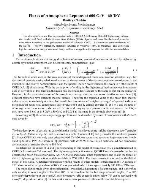
<strong>Fluxes</strong> <strong>of</strong> <strong>Atmospheric</strong> <strong>Leptons</strong> <strong>at</strong> <strong><strong>60</strong>0</strong> <strong>GeV</strong> - <strong>60</strong> TeV<br />
Dmitry Chirkin<br />
chirkin@physics.berkeley.edu<br />
University <strong>of</strong> California <strong>at</strong> <strong>Berkeley</strong>, USA<br />
Abstract<br />
The <strong>at</strong>mospheric muon flux is gener<strong>at</strong>ed with CORSIKA 6.030 (using QGSJET high-energy interaction<br />
model) and fitted with the formula from Gaisser (1990). Spectra and mass distribution <strong>of</strong> primaries<br />
were taken according to the poli-gon<strong>at</strong>o model <strong>of</strong> Hörandel (2003). A convenient parameteriz<strong>at</strong>ion <strong>of</strong><br />
the ¢¡¤£¦¥¨§© ¢¡¤£¦¥¨§© correction, originally tabul<strong>at</strong>ed in Volkova (1969), is presented. This correction,<br />
together with muon energy losses and decay, is shown to significantly improve the fit to the simul<strong>at</strong>ed d<strong>at</strong>a.<br />
1 Introduction<br />
The zenith-angle dependent energy distribution <strong>of</strong> muons, gener<strong>at</strong>ed in showers initi<strong>at</strong>ed by high-energy<br />
cosmic rays in the <strong>at</strong>mosphere, can be conveniently parametrized [1] as<br />
<br />
<br />
<br />
<br />
<strong>GeV</strong><br />
<br />
<br />
<br />
<br />
<br />
<br />
sr s <strong>GeV</strong> cm A <br />
This formula is <strong>of</strong>ten used in the d<strong>at</strong>a analyses <strong>of</strong> the underground muon and neutrino detectors, e.g., for<br />
the vertical depth-intensity rel<strong>at</strong>ion calcul<strong>at</strong>ion or the estim<strong>at</strong>es <strong>of</strong> the charm component contribution to the<br />
muon flux. The rel<strong>at</strong>ive normaliz<strong>at</strong>ion and the spectral index were varied in this work to fit the results <strong>of</strong><br />
CORSIKA [2] simul<strong>at</strong>ions. With the assumption <strong>of</strong> scaling in the high-energy hadron-nucleus interactions<br />
used in deriv<strong>at</strong>ion <strong>of</strong> this formula, the muon flux spectral index should be the same as th<strong>at</strong> for the primaries.<br />
However, in the parameteriz<strong>at</strong>ion <strong>of</strong> the cosmic ray energy spectrum and mass distribution used here [3],<br />
different primaries have different spectral indices. Therefore the expected value <strong>of</strong> the muon flux spectral<br />
index is not immedi<strong>at</strong>ely obvious, but should be close to some “weighted average” <strong>of</strong> spectral indices <strong>of</strong><br />
the individual cosmic ray components. In [4] values <strong>of</strong> and critical energies [5] <strong>at</strong><br />
<br />
(1)<br />
and the r<strong>at</strong>io <strong>of</strong><br />
to -gener<strong>at</strong>ed muons were also varied. In this work varying these parameters did not improve the fits, so<br />
<br />
they have been fixed <strong>at</strong> 115 <strong>GeV</strong>, 850 <strong>GeV</strong>, and 0.054 as indic<strong>at</strong>ed in the formula above (as in [1]).<br />
According to [3], the cosmic ray energy spectrum can be described by a sum <strong>of</strong> components with Z=1-92,<br />
each given by<br />
<br />
<br />
<br />
The best description <strong>of</strong> cosmic ray d<strong>at</strong>a within this model is achieved using rigidity-dependent<br />
¢<br />
<br />
cut<strong>of</strong>f energies<br />
. Values <br />
<strong>of</strong><br />
<br />
, , and , as well as a table <strong>of</strong> values <strong>of</strong> <br />
and used in this work are given<br />
<br />
in<br />
<br />
[3]. Since CORSIKA can only tre<strong>at</strong> primaries with Z=1-26, our cosmic ray spectrum implement<strong>at</strong>ion is only<br />
valid up to 50 PeV. As shown in [3], primaries with Z=28-92 as well as an additional ad-hoc component<br />
are important <strong>at</strong> energies above 100 PeV.<br />
To determine the values <strong>of</strong> and corresponding to this model <strong>of</strong> cosmic rays [3], a simul<strong>at</strong>ion based on<br />
CORSIKA version 6.030 was used. The high-energy interaction model QGSJET was shown to be the best to<br />
describe the muon fluxes observed by AMANDA [6] and several other experiments, and is also the fastest <strong>of</strong><br />
the six high-energy interaction models available in CORSIKA. For these reasons it was used as the default<br />
model in this work. A detailed comparison with the results <strong>of</strong> other models is presented in [6].<br />
<br />
A sample <strong>of</strong><br />
showers with energies above <strong><strong>60</strong>0</strong> <strong>GeV</strong> was gener<strong>at</strong>ed, which took approxim<strong>at</strong>ely<br />
<br />
200 GHz-CPU-days.<br />
The muon flux formula given above (Equ<strong>at</strong>ion 1) was derived assuming a fl<strong>at</strong> <strong>at</strong>mosphere, and<br />
<br />
is<br />
<br />
therefore<br />
only valid up to zenith angles <strong>of</strong> less than . In order to describe the full range <strong>of</strong> zenith<br />
<br />
angles, ,<br />
the dependence <strong>of</strong> the and critical energies valid <strong>at</strong> zenith <br />
angles below can be replaced ¦ with<br />
a dependence as in [5]. In this work a convenient parameteriz<strong>at</strong>ion <strong>of</strong> this substitution is ¤ given.<br />
1
2 The ¢¡¤£ ¥§¦©¨ ¢¡¤£ ¥§¦©¨ correction<br />
<br />
The muon flux formula as given in the previous section (Equ<strong>at</strong>ion 1) cannot be <br />
used for . In [5] the<br />
critical energies <strong>of</strong> and , here given simply as <br />
, ¦<br />
<br />
<br />
were calcul<strong>at</strong>ed taking into account the curv<strong>at</strong>ure <strong>of</strong> the <strong>at</strong>mosphere, thus extending the range <strong>of</strong> applicability<br />
to all zenith angles. The definition <strong>of</strong> the critical<br />
<br />
energy <strong>of</strong> or , i.e., the energy <strong>at</strong> which the or decay<br />
length is equal to the interaction length, is somewh<strong>at</strong> loose, and depends on the loc<strong>at</strong>ion <strong>of</strong> the first interaction<br />
<strong>of</strong> the cosmic ray primary. Its<br />
<br />
mean g/cm is estim<strong>at</strong>ed 85 in [5], and the average altitude<br />
as<br />
<br />
<strong>of</strong> muon<br />
production 17 km (for the direction ) in [7]. In this work, values 79.6 g/cm<br />
<strong>of</strong> as<br />
<br />
¤ <br />
¦ and <br />
19.28 km are obtained by comparison with CORSIKA-simul<strong>at</strong>ed muon flux above <strong><strong>60</strong>0</strong> <strong>GeV</strong> for the<br />
standard US <strong>at</strong>mosphere parameters (Figure 1), as shown in Figure 2.<br />
and<br />
X [ g/cm 2 ] and dX/dh<br />
10 -3 10 -2 10 -1<br />
10<br />
10<br />
1<br />
2<br />
10 3<br />
20<br />
18<br />
16<br />
14<br />
12<br />
10<br />
8<br />
6<br />
4<br />
2<br />
0<br />
h 0 [ km ] 10 -4<br />
Shib<strong>at</strong>a (from Gaisser, 1990)<br />
Standard US (as in CORSIKA)<br />
South Pole July 1 (CORSIKA)<br />
0 10 20 30 40 50 <strong>60</strong> 70 80 90 100<br />
0 10 20 30 40 50 <strong>60</strong> 70 80 90 100<br />
height [ km ]<br />
1/muon track length [ 10 -3 1/km ]<br />
70<br />
<strong>60</strong><br />
50<br />
40<br />
30<br />
20<br />
10<br />
model with X 0 =114.8 g/cm 2 , h 0 =19.28 m<br />
average muon track length from CORSIKA<br />
0<br />
0 0.1 0.2 0.3 0.4 0.5 0.6 0.7 0.8 0.9 1<br />
cos(θ)<br />
Figure 1: Model <strong>of</strong> the <strong>at</strong>mosphere. Figure 2: Muon track length.<br />
Assuming th<strong>at</strong> the interaction length <strong>of</strong> and in air<br />
<br />
<br />
<br />
<br />
<br />
is approxim<strong>at</strong>ely constant with energy, and the decay length is proportional<br />
energy,<br />
<br />
to <br />
<br />
Therefore, ¦ <br />
<br />
<br />
<br />
, the critical energy ) is (from<br />
<br />
§ <br />
<br />
<br />
<br />
<br />
<br />
<br />
<br />
<br />
<br />
<br />
<br />
Top <strong>of</strong> the <strong>at</strong>mosphere<br />
Earth surface<br />
<br />
At <br />
angles the <strong>at</strong>mosphere can be approxim<strong>at</strong>ed as fl<strong>at</strong><br />
<br />
and<br />
. The <strong>at</strong>mosphere above ¦ g/cm can be considered isothermal [1], therefore the density<br />
<br />
<br />
<br />
is proportional to the mass overburden<br />
<br />
above . The first interaction <strong>of</strong> <br />
a cosmic<br />
, <br />
<br />
2<br />
<br />
.<br />
θ<br />
x<br />
R<br />
θ *<br />
h
ay primary on average occurs <strong>at</strong> g/cm , where<br />
<br />
¡<br />
<br />
<br />
<br />
¡<br />
<br />
<br />
¦¤ ¢<br />
<br />
<br />
¤<br />
¡<br />
¢<br />
<br />
<br />
<br />
<br />
<br />
<br />
¦ (2)<br />
¦ . Therefore in this case ¦ ¤ . At larger angles can be approxim<strong>at</strong>ed as the<br />
zenith angle <strong>of</strong> the muon <strong>at</strong> the point <strong>of</strong> its production [7], as indic<strong>at</strong>ed in the figure above, since the integral<br />
i.e.<br />
in Equ<strong>at</strong>ion 2 is domin<strong>at</strong>ed by the contribution from the <strong>at</strong>mospheric layer with only<br />
<br />
£ <br />
a km,<br />
which can be considered approxim<strong>at</strong>ely fl<strong>at</strong>.<br />
<br />
width<br />
The altitude interaction, <strong>of</strong> the first , from<br />
<br />
can <br />
be determined <br />
¡<br />
, where<br />
<br />
<br />
<br />
<br />
¢¥¤ <br />
¨§©¥ <br />
¢ <br />
<br />
¢¥¤<br />
where is the radius <strong>of</strong> the Earth. This equ<strong>at</strong>ion was solved numerically<br />
<br />
for<br />
<br />
<br />
each and different <br />
<br />
<br />
. ¤ Then <br />
<br />
<br />
<br />
<br />
<br />
<br />
<br />
<br />
as well as the muon track length from the point <br />
<br />
production<br />
evalu<strong>at</strong>ed in this way are then averaged over depth muon weight <br />
<br />
production with .<br />
These averaged quantities can be fitted with<br />
<br />
¦ <br />
muon production altitude [ km ]<br />
40<br />
35<br />
30<br />
25<br />
20<br />
15<br />
<br />
¡<br />
¦<br />
<br />
can be calcul<strong>at</strong>ed. The quantities , , and<br />
<br />
¤ <br />
model with X 0 =114.8 g/cm 2 , h 0 =19.28 m<br />
3-parameter fit to the model (av. dev. 0.53%)<br />
5-parameter fit to the model (av. dev. 0.04%)<br />
model for the South Pole <strong>at</strong>mosphere<br />
0 0.1 0.2 0.3 0.4 0.5 0.6 0.7 0.8 0.9 1<br />
cos(θ)<br />
<br />
<br />
<br />
¥<br />
<br />
<br />
§©¥ <br />
<br />
<br />
<br />
<br />
<br />
<br />
<br />
cos(θ) *<br />
<br />
¥ <br />
<br />
1<br />
0.9<br />
0.8<br />
0.7<br />
0.6<br />
0.5<br />
0.4<br />
0.3<br />
0.2<br />
0.1<br />
<br />
<br />
<br />
<br />
<br />
<br />
<br />
<br />
model with X 0 =114.8 g/cm 2 , h 0 =19.28 m<br />
<br />
3-parameter fit to the model (av. dev. 0.24%)<br />
5-parameter fit to the model (av. dev. 0.20%)<br />
model for the South Pole <strong>at</strong>mosphere<br />
0<br />
0 0.1 0.2 0.3 0.4 0.5 0.6 0.7 0.8 0.9 1<br />
cos(θ)<br />
Figure 3: Average muon production altitude. Figure 4: ¤ parameteriz<strong>at</strong>ion.<br />
3
1/muon track length [ 10 -3 1/km ]<br />
70<br />
<strong>60</strong><br />
50<br />
40<br />
30<br />
20<br />
10<br />
model with X 0 =114.8 g/cm 2 , h 0 =19.28 m<br />
3-parameter fit to the model (av. dev. 0.46%)<br />
5-parameter fit to the model (av. dev. 0.40%)<br />
model for the South Pole <strong>at</strong>mosphere<br />
0<br />
0 0.1 0.2 0.3 0.4 0.5 0.6 0.7 0.8 0.9 1<br />
cos(θ)<br />
1/mass overburden [ 1/mwe ]<br />
0.12<br />
0.1<br />
0.08<br />
0.06<br />
0.04<br />
0.02<br />
model with X 0 =114.8 g/cm 2 , h 0 =19.28 m<br />
3-parameter fit to the model (av. dev. 1.17%)<br />
5-parameter fit to the model (av. dev. 0.20%)<br />
model for the South Pole <strong>at</strong>mosphere<br />
0<br />
0 0.1 0.2 0.3 0.4 0.5 0.6 0.7 0.8 0.9 1<br />
cos(θ)<br />
Figure 5: Average muon track length. Figure 6: Mass overburden <strong>of</strong> the <strong>at</strong>mosphere.<br />
and <br />
¥ <br />
<br />
<br />
. Additionally, the total <strong>at</strong>mospheric mass overburden as seen under zenith angle was<br />
where <br />
parametrized as<br />
¡ <br />
<br />
<br />
<br />
<br />
<br />
¥ <br />
<br />
<br />
All fits were first performed assuming the last two parameters are zero, and then another time allowing all<br />
five parameters to vary, as indic<strong>at</strong>ed in Figures 3-6. The five-parameter fits are accur<strong>at</strong>e to within better than<br />
0.40% and their parameters are summarized in Table 1.<br />
<br />
<br />
<br />
¢ <br />
<br />
fit av. devi<strong>at</strong>ion<br />
0.00851164 0.124534 0.059761 2.32876 19.279 0.04%<br />
¤ 0.102573 -0.068287 0.958633 0.0407253 0.817285 0.20%<br />
1.3144 50.2813 1.33545 0.252313 41.0344 0.40%<br />
¡ -0.017326 0.114236 1.15043 0.0200854 1.16714 0.20%<br />
Table 1: Parameters <strong>of</strong> the fits to the quantities , ¦ , , and ¡ <strong>of</strong> Section 2.<br />
The quantity ¦ was also calcul<strong>at</strong>ed as the zenith angle <strong>of</strong> the muon direction <strong>at</strong> the point <strong>of</strong> its<br />
production. As shown in Figure 7, the result is almost identical to the density r<strong>at</strong>io consider<strong>at</strong>ion. Also<br />
shown for comparison are the parameteriz<strong>at</strong>ions <strong>of</strong> [4].<br />
3 Muon energy losses and decay<br />
The muon integral flux <strong>at</strong> the muon production point £ is<br />
¤ <br />
<br />
¤ <br />
¡<br />
4
cos(θ ∗ )<br />
1<br />
0.9<br />
0.8<br />
0.7<br />
0.6<br />
0.5<br />
0.4<br />
0.3<br />
0.2<br />
0.1<br />
where <br />
the surface, ¤¡<br />
no correction<br />
density r<strong>at</strong>io model<br />
local muon cos(θ) model<br />
Klimushin et al. result<br />
with secθ correction<br />
0<br />
0 0.1 0.2 0.3 0.4 0.5 0.6 0.7 0.8 0.9 1<br />
cos(θ)<br />
total energy losses [ <strong>GeV</strong>/mwe ]<br />
10 4<br />
10 3<br />
10 2<br />
10<br />
1<br />
10 -1<br />
1/2 =a * +b * E<br />
a * =-0.487 [ <strong>GeV</strong>/mwe 1/2 ],<br />
b * =8.766 [ 10 -3 /mwe 1/2 ]<br />
10 3<br />
10 4<br />
=a+bE<br />
a=0.262 [ <strong>GeV</strong>/mwe ],<br />
b=0.350 [ 10 -3 /mwe ]<br />
10 5<br />
10<br />
energy [ <strong>GeV</strong> ]<br />
6<br />
Figure 7: ¦ parameteriz<strong>at</strong>ion. Figure 8: Muon energy loss parameters.<br />
<br />
<br />
is described by Equ<strong>at</strong>ion 1 with ¦¤ the correction <strong>of</strong> Section 2. The muon integral flux <strong>at</strong><br />
, can be calcul<strong>at</strong>ed from<br />
<br />
¤¡<br />
<br />
<br />
<br />
£¢<br />
<br />
¡<br />
¤¡<br />
<br />
<br />
<br />
£¢<br />
<br />
¡<br />
¤ ¤ <br />
where ¦¥ <br />
is determined by a stochastic process <strong>of</strong> muon propag<strong>at</strong>ion and depends on a random variable<br />
¤<br />
<br />
¦¥<br />
<br />
<br />
©<br />
. To determine the function with respect to all possible<br />
<br />
<br />
muon initial energies ¦¥<br />
On average, final energy <strong>of</strong> corresponds to some<br />
tion <strong>of</strong> the muon energy losses <br />
, <br />
where ¡ <br />
¦¥ <br />
<br />
¨§<br />
<br />
one must find the average <strong>of</strong> <br />
¤ <br />
which result in a muon final energy <strong>of</strong> .<br />
¥ ¤<br />
§ <br />
<br />
¥ ¤<br />
§ <br />
<br />
<br />
<br />
¤ ¤ <br />
<br />
<br />
¦¥ <br />
<br />
¨§ <br />
. Using the usual linear approxima-<br />
<br />
(3) <br />
Assuming th<strong>at</strong> the muon energy losses are small, the devi<strong>at</strong>ion <strong>of</strong> ¥<br />
¥ ¤<br />
from § its average can also be<br />
estim<strong>at</strong>ed. Using an approxim<strong>at</strong>ion<br />
¤ ¤ ¥ ¥ <br />
§ <br />
on a §¢ small p<strong>at</strong>h , and assuming th<strong>at</strong><br />
such devi<strong>at</strong>ions can be added p<strong>at</strong>h on a , one derives <br />
is the average mass overburden the muon crosses before reaching the surface.<br />
¤<br />
<br />
¥ ¤ ¥ §¢ § <br />
<br />
¢<br />
<br />
¤<br />
<br />
<br />
<br />
<br />
¢ <br />
¤<br />
<br />
Formulae 3 and 4 were used to fit a Monte Carlo simul<strong>at</strong>ion <strong>of</strong> muons propag<strong>at</strong>ing with energies <strong><strong>60</strong>0</strong> <strong>GeV</strong><br />
<strong>60</strong> TeV through 10 and 3<strong>60</strong> mwe <strong>of</strong> air performed with MMC [8]. Results <strong>of</strong> the fits are shown in Figure<br />
8. Dashed blue lines show the result <strong>of</strong> muon propag<strong>at</strong>ion through 10 mwe, and solid green lines through<br />
3<strong>60</strong> mwe, both rescaled to 1 mwe. The region <strong>of</strong> the fit is shown with vertical lines and the fits themselves<br />
5<br />
<br />
<br />
<br />
<br />
(4)
with solid light blue lines. A single set <br />
<strong>of</strong> ¤<br />
parameters and seems to describe well the<br />
devi<strong>at</strong>ions for both 10 and 3<strong>60</strong> mwe thus justifying the assumption <strong>of</strong> their additivity.<br />
It is now possible to derive the expression for ¤<br />
: <br />
¤¡<br />
<br />
<br />
¥ ¤<br />
§ <br />
<br />
<br />
¤<br />
<br />
<br />
<br />
<br />
¤ ¤ <br />
¤ ¥<br />
¥ <br />
<br />
¤ <br />
§¢<br />
<br />
<br />
<br />
¨§ <br />
¤ <br />
<br />
<br />
<br />
<br />
<br />
¤ ¤ <br />
¥ ¤<br />
§¢ <br />
¥ ¤<br />
§ <br />
¤<br />
<br />
<br />
¥ ¤ ¦¥ <br />
<br />
¥ ¤ ¥ §¢ § <br />
§¢ §<br />
<br />
¥ ¤ ¥ §¢ § <br />
<br />
¤ ¤ ¥ ¥<br />
¤ §¢ §¢ <br />
¤ <br />
§<br />
<br />
¡ <br />
<br />
<br />
<br />
Therefore, to account for the muon decay it is<br />
<br />
sufficient<br />
<br />
to replace in the formula from Section 1 with <br />
¤<br />
¤ ¥ <br />
<br />
. All quantities <strong>of</strong> this section (including the deriv<strong>at</strong>ive<br />
¡ <br />
. Additionally, £¢ ¡<br />
<br />
<br />
<br />
) can easily be evalu<strong>at</strong>ed and are implemented in the function fitted to the ¡ muon spectrum.<br />
Muon decay is factor <br />
¥¤ evalu<strong>at</strong>ed as ¡ a correction . <br />
4 Fits to the muon energy spectrum <strong>at</strong> the surface<br />
The fit to Formula 1 is shown in Figure 9, and to the corrected formula in Figure 10. Both figures<br />
¨§ <br />
show<br />
and in the full<br />
¦ ¤<br />
<br />
. the fit as a function ¦ <strong>of</strong><br />
¤<br />
parameters <strong>of</strong> the fit and as well as the <strong>of</strong> the fit in the region <strong>of</strong><br />
range Figure 11 shows the behavior <strong>of</strong> the parameters and <strong>of</strong><br />
the lower boundary <strong>of</strong> the fit, the upper boundary always <strong>at</strong> ¤<br />
. Equ<strong>at</strong>ion 1 can only be used for<br />
¨§<br />
, as mentioned before, and gives the same result in this region as the ¤ -only corrected<br />
¦¤<br />
formula. Both approaches fail to produce values <strong>of</strong> the fit parameters independent <strong>of</strong> the region <strong>of</strong> the fit.<br />
Including muon energy losses substantially improves the fit. Additionally correcting for muon decay gives<br />
the best description <strong>of</strong> the muon spectra. The value<br />
<br />
<br />
§<br />
<strong>of</strong> drops to 1.2 <strong>at</strong> lower boundary ©¨ <strong>of</strong> ¦<br />
and is 1.12 <strong>at</strong> ¦© <br />
<br />
and<br />
¤ ¤<br />
<strong>at</strong> ¦©¨ <br />
10 5<br />
10 4<br />
10 3<br />
10 2<br />
10<br />
Φ 0 = 0.14 cm -2 s -1 sr -1 ⋅ A<br />
χ 2 =1106.08 (cosθ=0-1)<br />
qgsjet<br />
10 3<br />
E [<strong>GeV</strong>]<br />
10 4<br />
0<br />
¨§ . The values <strong>of</strong> and vary very little as the region <strong>of</strong> the fit changes, and are<br />
0.2<br />
¨§ .<br />
0.4<br />
0.6<br />
A<br />
γ<br />
χ 2<br />
= 0.595<br />
= 2.697<br />
= 3.13<br />
0.8<br />
cos(θ)<br />
Figure 9: Fit with Formula 1 to the CORSIKAsimul<strong>at</strong>ed<br />
muon energy spectrum.<br />
1<br />
6<br />
10 5<br />
10 4<br />
10 3<br />
10 2<br />
10<br />
Φ 0 = 0.14 cm -2 s -1 sr -1 ⋅ A<br />
χ 2 =49.94 (cosθ=0-1)<br />
qgsjet<br />
10 3<br />
E [<strong>GeV</strong>]<br />
10 4<br />
0<br />
0.2<br />
0.4<br />
0.6<br />
A<br />
γ<br />
χ 2<br />
= 0.701<br />
= 2.715<br />
= 1.12<br />
0.8<br />
cos(θ)<br />
Figure 10: Fit with the corrected Formula 1.<br />
1
The resulting muon differential flux <strong>at</strong> 10 TeV is plotted in Figure 12, which can be compared with a<br />
figure containing results <strong>of</strong> different approaches to ¦¤ calcul<strong>at</strong>ion <strong>of</strong> from [7]. Resulting fits to the muon<br />
integral fluxes are shown in Figures 13 and 14. CORSIKA-simul<strong>at</strong>ed muon energy spectra appear to have<br />
some unexpected ¦<br />
§<br />
structure <strong>at</strong> , which causes ¦ <br />
<br />
a high <strong>of</strong> the fit to the whole<br />
<br />
region <strong>of</strong><br />
. This was noticed before [9], but was shown not to affect the simul<strong>at</strong>ion <strong>of</strong> the muon flux <strong>at</strong> the<br />
depth <strong>of</strong> AMANDA-II (1730 m) or deeper. The highest value <strong>of</strong> the zenith angle <strong>at</strong> the surface which can be<br />
¦¤<br />
seen <strong>at</strong> the depth <strong>of</strong> AMANDA-II is 88.7 § <br />
, i.e. , where the artifact is much less pronounced.<br />
<br />
γ<br />
A<br />
χ 2<br />
2.74<br />
2.72<br />
2.7<br />
2.68<br />
2.66<br />
original formula<br />
+cos(θ)-correction<br />
+dE/dx losses<br />
+muon decay<br />
0 0.1 0.2 0.3 0.4 0.5 0.6 0.7 0.8 0.9 1<br />
0.7<br />
0.65<br />
0.6<br />
0.55<br />
0.5<br />
0 0.1 0.2 0.3 0.4 0.5 0.6 0.7 0.8 0.9 1<br />
10 2<br />
10<br />
1<br />
1<br />
0 0.1 0.2 0.3 0.4 0.5 0.6 0.7 0.8 0.9 1<br />
lower cos(θ) bound in fits<br />
2<br />
I(cos(θ)) / I(cos(θ)=1) <strong>at</strong> 10 TeV<br />
12<br />
10<br />
8<br />
6<br />
4<br />
2<br />
no correction<br />
cos(θ)-correction only<br />
fit with the corrected formula<br />
for the South Pole July <strong>at</strong>mosphere<br />
0<br />
0 0.1 0.2 0.3 0.4 0.5 0.6 0.7 0.8 0.9 1<br />
cos(θ)<br />
Figure 11: Behavior <strong>of</strong> the parameters <strong>of</strong> the fit. Figure 12: Muon differential flux <strong>at</strong> 10 TeV.<br />
5 Uncertainties in the fit model<br />
To investig<strong>at</strong>e the effect <strong>of</strong> the uncertainties in the knowledge <strong>of</strong> the <strong>at</strong>mospheric pr<strong>of</strong>ile, the standard US<br />
<strong>at</strong>mosphere used in the fits <strong>of</strong> Section 2 was replaced with the winter (July) <strong>at</strong>mosphere <strong>at</strong> the South Pole (see<br />
Figure 1 for comparison with standard US <strong>at</strong>mosphere). The ground level for this South Pole <strong>at</strong>mosphere was<br />
chosen <strong>at</strong> 115.5 m below the see level to m<strong>at</strong>ch the <strong>at</strong>mospheric pressure <strong>at</strong> ground with th<strong>at</strong> <strong>of</strong> the Standard<br />
US <strong>at</strong>mosphere. As seen from Figures 3-6, only the average muon production altitude and the muon track<br />
length undergo substantial changes. As seen from Figure 4, the change in the average muon production does<br />
not affect the ¤ calcul<strong>at</strong>ion. Most <strong>of</strong> the muon decays occur for muons with the longest tracks, which<br />
come from near the horizon. There the devi<strong>at</strong>ion in the track length from th<strong>at</strong> calcul<strong>at</strong>ed for the standard US<br />
<strong>at</strong>mosphere is small, as seen from Figure 5. Therefore, quantities parameterized in Section 2 for the standard<br />
US <strong>at</strong>mosphere can be used for the <strong>at</strong>mosphere with quite different pr<strong>of</strong>ile, in the extreme case the winter<br />
<strong>at</strong>mosphere <strong>at</strong> the South Pole.<br />
Fits <strong>of</strong> the previous section were calcul<strong>at</strong>ed to the CORSIKA-simul<strong>at</strong>ed muon d<strong>at</strong>a gener<strong>at</strong>ed in the absence<br />
<strong>of</strong> the magnetic field. As seen from Figure 16, adding a 50 nT magnetic field changes the muon<br />
sc<strong>at</strong>tering pr<strong>of</strong>ile. The sc<strong>at</strong>tering width is 2-4 times th<strong>at</strong> without the magnetic field, but is still very small for<br />
muons with energies above <strong><strong>60</strong>0</strong> <strong>GeV</strong>.<br />
Fit parameters for both a wrong <strong>at</strong>mospheric pr<strong>of</strong>ile and a non-zero magnetic field are shown in Figure 15.<br />
As expected, the change from the calcul<strong>at</strong>ion <strong>of</strong> Section 4 is negligible. However, the parameters do change<br />
somewh<strong>at</strong> when the fits are recalcul<strong>at</strong>ed in the energy range 1-100 TeV.<br />
7
Muon flux above <strong><strong>60</strong>0</strong> <strong>GeV</strong> [ 10 -6 cm -1 sr -1 s -1 ]<br />
γ<br />
A<br />
χ 2<br />
0.6<br />
0.5<br />
0.4<br />
0.3<br />
0.2<br />
0.1<br />
CORSIKA muon integr<strong>at</strong>ed flux<br />
fit with the corrected formula<br />
fit with the original formula<br />
fit with cos(θ)-correction only<br />
0<br />
0 0.1 0.2 0.3 0.4 0.5 0.6 0.7 0.8 0.9 1<br />
cos(θ)<br />
Muon flux above 10 TeV [ 10 -9 cm -1 sr -1 s -1 ]<br />
0.7<br />
0.6<br />
0.5<br />
0.4<br />
0.3<br />
0.2<br />
0.1<br />
CORSIKA muon integr<strong>at</strong>ed flux<br />
fit with the corrected formula<br />
fit with the original formula<br />
fit with cos(θ)-correction only<br />
0<br />
0 0.1 0.2 0.3 0.4 0.5 0.6 0.7 0.8 0.9 1<br />
cos(θ)<br />
Figure 13: Integr<strong>at</strong>ed muon flux <strong>at</strong> <strong><strong>60</strong>0</strong> <strong>GeV</strong>. Figure 14: Integr<strong>at</strong>ed muon flux <strong>at</strong> 10 TeV.<br />
2.73<br />
2.72<br />
2.71<br />
fit in 1-100 TeV<br />
with SP Jul <strong>at</strong>m<br />
w/magnetic field<br />
corrected formula<br />
2.7<br />
0 0.1 0.2 0.3 0.4 0.5 0.6 0.7 0.8 0.9 1<br />
0.74<br />
0.72<br />
0.7<br />
0.68<br />
10<br />
0 0.1 0.2 0.3 0.4 0.5 0.6 0.7 0.8 0.9 1<br />
1<br />
1<br />
0 0.1 0.2 0.3 0.4 0.5 0.6 0.7 0.8 0.9 1<br />
lower cos(θ) bound in fits<br />
1.2<br />
devi<strong>at</strong>ion in θ from direction <strong>of</strong> primary [ ° ]<br />
1<br />
0.8<br />
0.6<br />
0.4<br />
0.2<br />
0<br />
-0.2<br />
-0.4<br />
-0.6<br />
-0.8<br />
θ color map:<br />
with magnetic field:<br />
no magnetic field:<br />
-1<br />
-1 -0.8 -0.6 -0.4 -0.2 0 0.2 0.4 0.6 0.8 1<br />
devi<strong>at</strong>ion in φ from direction <strong>of</strong> primary [ ° ]<br />
Figure 15: Uncertainties in the fit parameters. Figure 16: Magnetic field influence.<br />
6 Energy spectra <strong>of</strong> <strong>at</strong>mospheric muon and electron neutrinos<br />
Along with muons, CORSIKA gener<strong>at</strong>es muon and electron neutrinos, spectra <strong>of</strong> which were fitted with<br />
the formulae from [10]. Muon neutrino spectra were fitted with<br />
<br />
<br />
<br />
cm sr s <strong>GeV</strong> A <br />
<br />
<br />
<br />
<br />
<strong>GeV</strong><br />
8<br />
<br />
¤£ ¦¥ ¢¡<br />
<br />
<br />
θ<br />
§ <br />
¤£ ¦¥<br />
¨§©
and electron neutrino spectra were fitted with<br />
<br />
¢¥¤ §¦ ¨<br />
<br />
<br />
cm sr s <strong>GeV</strong> A <br />
<br />
<br />
<br />
<br />
<br />
<br />
¡<br />
<strong>GeV</strong> <br />
<br />
£ ¦¥ <br />
¨§© <br />
<br />
©<br />
£ <br />
¦ <br />
<br />
<br />
<br />
£ ¦¥ <br />
§ <br />
<br />
© £ <br />
<br />
<br />
£¢ ¡ <br />
£ ¦¥<br />
<br />
<br />
¨§<br />
¦ ¦¤ <br />
The muon neutrino energy spectrum fit demonstr<strong>at</strong>es the same stability with respect to changes in the<br />
¦¤© lower boundary <strong>of</strong> the fit as the muon energy spectrum fit. Electron neutrino fit parameters, however,<br />
change in the range<br />
shown in Figures 17 and 18 were produced with ©¨ <br />
10 5<br />
10 4<br />
10 3<br />
10 2<br />
10<br />
Φ 0 = 0.0285 cm -2 s -1 sr -1 ⋅ A<br />
χ 2 = 1.10 (cosθ=0-1)<br />
qgsjet<br />
10 3<br />
E [<strong>GeV</strong>]<br />
10 4<br />
0<br />
¦ ¦<br />
£ § §<br />
¦¤© ¨§ and as is varied from 0 to 0.5. The fits<br />
.<br />
0.2<br />
0.4<br />
0.6<br />
A<br />
γ<br />
χ 2<br />
= 0.646<br />
= 2.684<br />
= 1.08<br />
0.8<br />
cos(θ)<br />
1<br />
Φ 0 = 0.0024 cm -2 s -1 sr -1 ⋅ A<br />
χ 2 = 2.01 (cosθ=0-1)<br />
10 3<br />
E [<strong>GeV</strong>]<br />
10 4<br />
0<br />
0.2<br />
0.4<br />
0.6<br />
0.8<br />
§<br />
A<br />
γ<br />
χ 2<br />
= 0.828<br />
= 2.710<br />
= 1.17<br />
cos(θ)<br />
Figure 17: Muon neutrino energy spectrum fit. Figure 18: Electron neutrino energy spectrum fit.<br />
7 Results and Conclusions<br />
Muon and muon- and electron neutrino energy spectra produced with CORSIKA in the energy range <strong><strong>60</strong>0</strong><br />
<strong>GeV</strong> <strong>60</strong> TeV were fitted with Formula 1 after a ¦¤ correction as described in Section 2 (see Table 2).<br />
Muon spectra fits were additionally corrected for the muon energy losses and decay. These corrections were<br />
shown to be important in the selected energy range. Convenient parameteriz<strong>at</strong>ions <strong>of</strong> ¦ correction and<br />
muon energy losses were given.<br />
10 5<br />
10 4<br />
10 3<br />
10 2<br />
10<br />
qgsjet<br />
<br />
<br />
<br />
0.701 0.006 0.646 0.003 0.828 0.155<br />
2.715 0.001 2.684 0.001 2.710 0.023<br />
¤ <br />
Table 2: Muon and muon- and electron neutrino energy spectrum parameters.<br />
9<br />
<br />
1
References<br />
[1] Gaisser, T.K. 1990, Cosmic Rays and Particle Physics, Cambridge<br />
[2] Heck, D., et al., CORSIKA: A Monte Carlo Code to Simul<strong>at</strong>e Extensive Air Showers, physics manual<br />
distributed together with CORSIKA sources<br />
[3] Hörandel, J., Astropart. Phys. 19 (2003) 193<br />
[4] Klimushin, S., Bugaev, E., & Sokalski, I., Analytical description <strong>of</strong> muon distributions <strong>at</strong> large depths,<br />
27th ICRC, Hamburg, 2001<br />
[5] Volkova, L. V., Lebedev Physical Institute Report No. 72, 1969<br />
[6] Chirkin, D.A., Cosmic Ray Energy Spectrum Measurement with the Antarctic Muon and Neutrino<br />
Detector Array (AMANDA), 2003, Ph.D. thesis, UC <strong>Berkeley</strong><br />
[7] Aglietta, M., et al., LVD Coll., Upper Limit on the prompt muon flux derived from the LVD underground<br />
experiment, Phys. Rev. D, Vol. <strong>60</strong>, 112001, 1999<br />
[8] mmc code homepage is http://amanda.berkeley.edu/˜dima/work/MUONPR/<br />
mmc code available <strong>at</strong> http://amanda.berkeley.edu/˜dima/work/MUONPR/BKP/mmc.tgz<br />
[9] dCORSIKA upd<strong>at</strong>e report: http://amanda.berkeley.edu/˜dima/work/BKP/DCS/REPORT8/paper.ps.gz<br />
[10] Volkova, L.V. 1980, Sov. J. Nucl. Phys. 31, 784<br />
10