Economics - Cengage Learning

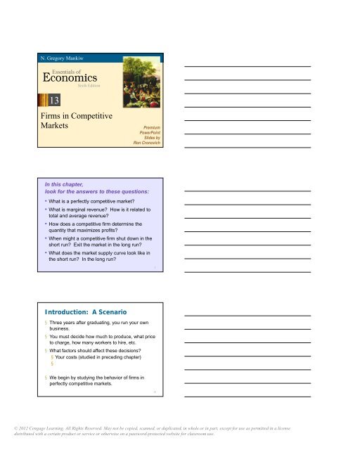
N. Gregory Mankiw
Essentials of
Economics
Sixth Edition
13
Firms in Competitive
Markets Premium
PowerPoint
Slides by
Ron Cronovich
In this chapter,
look for the answers to these questions:
• What is a perfectly competitive market?
• What is marginal revenue? How is it related to
total and average revenue?
• How does a competitive firm determine the
quantity that maximizes profits?
• When might a competitive firm shut down in the
short run? Exit the market in the long run?
• What does the market supply curve look like in
the short run? In the long run?
Introduction: A Scenario
§ Three years after graduating, you run your own
business.
§ You must decide how much to produce, what price
to charge, how many workers to hire, etc.
§ What factors should affect these decisions?
§ Your costs (studied in preceding chapter)
§
§ We begin by studying the behavior of firms in
perfectly competitive markets.
© 2012 CengageLearning. All Rights Reserved. May not be copied, scanned, or duplicated, in whole or in part, except for use as permitted in alicense
distributed with a certain product or service or otherwise on a password-protected website for classroom use.
1
2

Characteristics of Perfect Competition
1.
2.
3.
§ Because of 1 & 2, each buyer and seller is a
The Revenue of a Competitive Firm
§ Total revenue (TR)
§ Average revenue (AR)
§ Marginal revenue (MR):
ACTIVE LEARNING 1
Calculating TR, AR, MR
Fill in the empty spaces of the table.
Q P TR AR MR
0
1
2
3
4
5
$10
$10
$10
$10
$10
$10
$40
$50
n/a
$10
$10
© 2012 CengageLearning. All Rights Reserved. May not be copied, scanned, or duplicated, in whole or in part, except for use as permitted in alicense
distributed with a certain product or service or otherwise on a password-protected website for classroom use.
3
4

MR = P for a Competitive Firm
§ A competitive firm can keep increasing its output
without affecting the market price.
§ So, each one-unit increase in Q causes revenue
to rise by
Profit Maximization
§ What Q maximizes the firm’s profit?
§ To find the answer, “think at the margin.”
If increase Q by one unit,
§ If MR > MC, then
§ If MR < MC, then
Profit Maximization
At any Q with
MR > MC,
increasing Q
raises profit.
At any Q with
MR < MC,
reducing Q
raises profit.
(continued from earlier exercise)
Q
0
1
2
3
4
5
TR
$0
10
20
30
40
50
TC
$5
9
15
23
33
45
Profit
–$5
1
5
7
7
5
MR
$10
10
10
10
10
MC
$4
6
8
10
12
© 2012 CengageLearning. All Rights Reserved. May not be copied, scanned, or duplicated, in whole or in part, except for use as permitted in alicense
distributed with a certain product or service or otherwise on a password-protected website for classroom use.
7
8
DProfit =
MR – MC
$6
4
2
0
–2
9

MC and the Firm’s Supply Decision
At Q a,
At Q b,
At Q 1,
Costs
P 1
MC
MC and the Firm’s Supply Decision
If price rises to P 2,
then the profitmaximizing
quantity
The MC curve
determines the
firm’s Q at any price.
Hence,
Costs
P 1
Shutdown vs. Exit
§ Shutdown:
§ Exit:
§ A key difference:
Q 1
MC
MR
Q
MR
Q
10
11
12
© 2012 CengageLearning. All Rights Reserved. May not be copied, scanned, or duplicated, in whole or in part, except for use as permitted in alicense
distributed with a certain product or service or otherwise on a password-protected website for classroom use.

A Firm’s Short-run Decision to Shut Down
§ Cost of shutting down:
§ Benefit of shutting down:
§ So, shut down if
§ Divide both sides by Q:
§ So, firm’s decision rule is:
A Competitive Firm’s SR Supply Curve
If P > AVC, then
firm produces Q
where P = MC.
If P < AVC, then
firm shuts down
(produces Q = 0).
Costs
The Irrelevance of Sunk Costs
§ Sunk cost:
MC
ATC
AVC
§ Sunk costs should be irrelevant to decisions;
you must pay them regardless of your choice.
§ FC is a sunk cost: The firm must pay its fixed
costs whether it produces or shuts down.
§ So,
Q
13
14
15
© 2012 CengageLearning. All Rights Reserved. May not be copied, scanned, or duplicated, in whole or in part, except for use as permitted in alicense
distributed with a certain product or service or otherwise on a password-protected website for classroom use.

A Firm’s Long-Run Decision to Exit
§ Cost of exiting the market:
§ Benefit of exiting the market:
§ So, firm exits if
§ Divide both sides by Q to write the firm’s
decision rule as:
A New Firm’s Decision to Enter Market
§ In the long run, a new firm will enter the market if
it is profitable to do so:
§ Divide both sides by Q to express the firm’s
entry decision as:
The Competitive Firm’s Supply Curve
The firm’s
LR supply curve
is
Costs
MC
Q
16
17
LRATC
18
© 2012 CengageLearning. All Rights Reserved. May not be copied, scanned, or duplicated, in whole or in part, except for use as permitted in alicense
distributed with a certain product or service or otherwise on a password-protected website for classroom use.

ACTIVE LEARNING 2
Identifying a firm’s profit
Determine
this firm’s
total profit.
Identify the
area on the
graph that
represents
the firm’s
profit.
Costs, P
MC
P = $10 MR
ATC
$6
ACTIVE LEARNING 3
Identifying a firm’s loss
Determine
this firm’s
total loss,
assuming
AVC < $3.
Identify the
area on the
graph that
represents
the firm’s
loss.
Costs, P
$5
A competitive firm
50
A competitive firm
MC
Q
ATC
P = $3 MR
30
Market Supply: Assumptions
1) All existing firms and potential entrants
2) Each firm’s costs
3) The number of firms in the market is
§ ______________ in the short run
due to
§ ______________ in the long run
due to
Q
23
© 2012 CengageLearning. All Rights Reserved. May not be copied, scanned, or duplicated, in whole or in part, except for use as permitted in alicense
distributed with a certain product or service or otherwise on a password-protected website for classroom use.

The SR Market Supply Curve
§ As long as P ≥ AVC, each firm will produce its
profit-maximizing quantity
§ Recall from Chapter 4:
At each price, the market quantity supplied is
the sum of quantities supplied by all firms.
The SR Market Supply Curve
Example: 1000 identical firms
At each P, market Q s = 1000 x (one firm’s Q s )
P 1
P
10
One firm
MC
AVC
Q
(firm)
P 1
P
10,000
Market
Entry & Exit in the Long Run
S
24
Q
(market)
§ In the LR, the number of firms can change due
to entry & exit.
§ If existing firms earn positive economic profit,
§ If existing firms incur losses,
25
26
© 2012 CengageLearning. All Rights Reserved. May not be copied, scanned, or duplicated, in whole or in part, except for use as permitted in alicense
distributed with a certain product or service or otherwise on a password-protected website for classroom use.

The Zero-Profit Condition
§ Long-run equilibrium:
The process of
§ Zero economic profit occurs when
§ Since firms produce where
the zero-profit condition is
§ Recall that MC intersects ATC at minimum ATC.
§ Hence, in the long run,
Why Do Firms Stay in Business
if Profit = 0?
§ Recall, economic profit is revenue minus all costs,
including
§ In the zero-profit equilibrium,
The LR Market Supply Curve
In the long run,
the typical firm
earns zero profit.
P =
min.
ATC
P
One firm
MC
LRATC
Q
(firm)
P
Market
27
28
Q
(market)
29
© 2012 CengageLearning. All Rights Reserved. May not be copied, scanned, or duplicated, in whole or in part, except for use as permitted in alicense
distributed with a certain product or service or otherwise on a password-protected website for classroom use.

SR & LR Effects of an Increase in Demand
P 1
P
One firm
MC
ATC
Q
(firm)
P 1
P
Market
S 1
long-run
supply
D1 Q
(market)
Why the LR Supply Curve Might Slope Upward
§ The LR market supply curve is horizontal if
A
Q 1
1) all firms have identical costs, and
2) costs do not change as other firms enter or
exit the market.
§ If either of these assumptions is not true,
then LR supply curve slopes upward.
1) Firms Have Different Costs
§ As P rises, firms with lower costs enter the market
before those with higher costs.
§ Further increases in
§ Hence, LR market supply curve slopes upward.
§ At any P,
§ For the marginal firm,
§ For lower-cost firms,
30
31
32
© 2012 CengageLearning. All Rights Reserved. May not be copied, scanned, or duplicated, in whole or in part, except for use as permitted in alicense
distributed with a certain product or service or otherwise on a password-protected website for classroom use.

2) Costs Rise as Firms Enter the Market
§ In some industries,
§ The entry of new firms
§
§ Hence, an increase in P is required to increase
the market quantity supplied, so the supply
curve is upward-sloping.
CONCLUSION:
The Efficiency of a Competitive Market
§ Profit-maximization:
§ Perfect competition:
§ So, in the competitive eq’m:
§ Recall, MC is cost of producing the marginal unit.
P is value to buyers of the marginal unit.
§ So,
§ In the next chapter, monopoly: pricing and
production decisions, deadweight loss, regulation.
33
34
© 2012 CengageLearning. All Rights Reserved. May not be copied, scanned, or duplicated, in whole or in part, except for use as permitted in alicense
distributed with a certain product or service or otherwise on a password-protected website for classroom use.