Tropical Combinatorics
Tropical Combinatorics
Tropical Combinatorics

Create successful ePaper yourself
Turn your PDF publications into a flip-book with our unique Google optimized e-Paper software.
<strong>Tropical</strong> <strong>Combinatorics</strong><br />
Michael Joswig<br />
TU Darmstadt<br />
Bertinoro, Sep 28–30, 2009
1 <strong>Tropical</strong> Hypersurfaces<br />
The tropical semi-ring<br />
Polyhedral combinatorics<br />
Puiseux series<br />
2 <strong>Tropical</strong> Convexity<br />
<strong>Tropical</strong> polytopes<br />
Type decomposition<br />
Products of simplices<br />
3 Resolution of Monomial Ideals<br />
The coarse type ideal<br />
(Co)-cellular resolutions<br />
Overview
tropical semi-ring: (R ∪ {+∞}, ⊕, ⊙) where<br />
x ⊕ y := min(x, y) and x ⊙ y := x + y<br />
<strong>Tropical</strong> Arithmetic<br />
Example<br />
(3 ⊕ 5) ⊙ 2 = 3 + 2 = 5 = min(5, 7) = (3 ⊙ 2) ⊕ (5 ⊙ 2)<br />
History<br />
can be traced back (at least) to the 1960s<br />
e.g., see monography [Cunningham-Green 1979]<br />
optimization, functional analysis, signal processing, . . .<br />
recent development (since 2002) initiated by Kapranov,<br />
Mikhalkin, Sturmfels, . . .
<strong>Tropical</strong> Polynomials<br />
read ordinary (Laurent) polynomial with real coefficients as<br />
function<br />
replace operations “+” and “·” by “⊕” and “⊙”<br />
Example<br />
F(x) := (7 ⊙ x ⊙3 ) ⊕ (3 ⊙ x) ⊕ 4 = min(7 + 3x,3 + x,4)<br />
Definition<br />
tropical polynomial F vanishes at p :⇔ there are at least two<br />
terms where the minimum F(p) is attained<br />
F(1) = min(7 + 3 · 1, 3+1 , 4 ) = 4
tropical semi-module (R d , ⊕, ⊙)<br />
componentwise addition<br />
tropical scalar multiplication<br />
<strong>Tropical</strong> Hypersurfaces<br />
Definition<br />
tropical hypersurface T (F) := vanishing locus of (multi-variate)<br />
tropical polynomial F<br />
Example<br />
F(x) = (7 ⊙ x ⊙3 ) ⊕ (3 ⊙ x) ⊕ 4<br />
T (F) = {−2, 1} ⊂ R 1<br />
(−2,1)<br />
−2 1<br />
7 + 3x<br />
(1,4)<br />
3 + x<br />
4
Polyhedral <strong>Combinatorics</strong><br />
Proposition<br />
For a tropical polynomial F : Rd → R the set<br />
<br />
P(F) := (p, s) ∈ R d+1 : p ∈ R d <br />
, s ∈ R, s ≤ F(p)<br />
is an unbounded convex polyhedron of dimension d + 1.<br />
Corollary<br />
The tropical hypersurface T (F) coincides with the image of the<br />
codimension-2-skeleton of the polyhedron P(F) in R d under the<br />
orthogonal projection which omits the last coordinate.
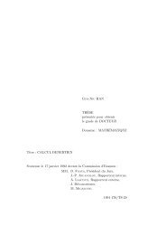
The Newton Polytope of a <strong>Tropical</strong> Polynomial<br />
Definition<br />
Newton polytope N(F) = convex hull of the support supp(F)<br />
Theorem<br />
The tropical hypersurface T (F) of a tropical polynomial F is dual<br />
to the 1-coskeleton of the regular subdivision of N(F) induced by<br />
the coefficients of F.<br />
(−2,1)<br />
7 + 3x<br />
−2 1<br />
(1,4)<br />
3 + x<br />
4<br />
(0,4)<br />
(1,3)<br />
0 1 3<br />
(3,7)
The <strong>Tropical</strong> Torus<br />
tropical polynomial F homogeneous of degree δ if for all p ∈ R d<br />
and λ ∈ R:<br />
F(λ ⊙ p) = F(λ · 1 + p) = λ ⊙δ ⊙ F(p) = δ · λ + F(p)<br />
Definition<br />
tropical (d − 1)-torus T d−1 := R d /R1<br />
map<br />
(x1, x2, . . .,xd) + R1 = (0, x2 − x1, . . .,xd − x1) + R1<br />
defines homeomorphism T d−1 ≈ R d−1<br />
↦→ (x2 − x1, . . .,xd − x1)
<strong>Tropical</strong> Hyperplanes<br />
F(x) = (α1 ⊙ x1) ⊕ (α2 ⊙ x2) ⊕ (α3 ⊙ x3) linear homogeneous<br />
T (F) = −(α1, α2, α3) + (R≥0e1 ∪ R≥0e2 ∪ R≥0e3) + R1<br />
= (0, α1 − α2, α1 − α3) + (R≥0(−e2 − e3) ∪ R≥0e2 ∪ R≥0e3)<br />
−α
general tropical conic<br />
<strong>Tropical</strong> Conics<br />
(a200 ⊙ x ⊙2<br />
1 ) ⊕ (a110 ⊙ x1 ⊙ x2) ⊕ (a101 ⊙ x1 ⊙ x3)<br />
⊕ (a020 ⊙ x ⊙2<br />
2 ) ⊕ (a011 ⊙ x2 ⊙ x3) ⊕ (a002 ⊙ x ⊙2<br />
3 )<br />
Example<br />
(a200, a110, a101, a020, a011, a002) = (6, 5, 5, 6, 5, 7)<br />
4<br />
3<br />
2<br />
1<br />
0<br />
-1<br />
-2<br />
-3<br />
-4 -4<br />
-3<br />
-2<br />
-1<br />
3 2<br />
0<br />
4<br />
1<br />
1<br />
2<br />
3<br />
4<br />
(2,0,0)<br />
1<br />
(1,1,0) (1,0,1)<br />
2<br />
3 4<br />
(0,2,0) (0,1,1) (0,0,2)
duality between min and max:<br />
Max-<strong>Tropical</strong> Hyperplanes<br />
max(−x, −y) = −min(x, y)<br />
Remark<br />
T is min-tropical hyperplane ⇐⇒ −T is max-tropical hyperplane<br />
−α α<br />
min/max
Puiseux series with complex coefficients:<br />
<br />
∞<br />
C{{z}} =<br />
k=m<br />
Fields of Puiseux Series<br />
ak · z k/N : m ∈ Z, N ∈ N × , ak ∈ C<br />
Newton-Puiseux-Theorem: C{{z}} isomorphic to algebraic<br />
closure of Laurent series C((z))<br />
isomorphic to C by [Steinitz 1910]
valuation map<br />
val : C{{z}} → Q ∪ {∞}<br />
The Valuation Map<br />
maps Puiseux series γ(z) = ∞<br />
k=m ak · z k/N to lowest degree<br />
min{k/N : k ∈ Z, ak = 0}; setting val(0) := ∞<br />
val(γ(z) + δ(z)) ≥ min{val(γ(z)), val(δ(z))}<br />
val(γ(z) · δ(z)) = val(γ(z)) + val(δ(z)).<br />
Remark<br />
inequality becomes equation if no cancellation occurs
A Lifting Theorem I<br />
Theorem (Einsiedler, Kapranov & Lind 2006)<br />
For f ∈ K[x ±1<br />
1 , x±1 2 , . . .,x±1 d ] the tropical hypersurface<br />
T (trop(f)) ∩ Qd (over the rationals) equals the set val(V (〈f〉)).<br />
<strong>Tropical</strong> geometry is a piece-wise linear shadow of<br />
classical geometry.
A Lifting Theorem II<br />
Proof of easy inclusion “T (trop(f)) ⊇ val(V (〈f〉))”.<br />
let f = <br />
i∈I γix i for I ⊂ N d with tropicalization F<br />
consider zero u ∈ (K × ) d of f<br />
for i ∈ I we have<br />
val(γiu i ) = val(γi) + 〈i,val(u)〉 = val(γi) ⊙ val(u) ⊙i<br />
minimum<br />
F(val(u)) = <br />
val(γi) ⊙ val(u) ⊙i<br />
i∈I<br />
attained at least twice since otherwise the terms γiu i cannot<br />
cancel to yield zero
tropicalization of (homogeneous) polynomial F<br />
tropical hypersurface T (F)<br />
codimension-2-skeleton of unbounded convex polyhedron<br />
regular subdivision of Newton polytope N(F)<br />
Conclusion I<br />
tropical hypersurface = image of ordinary hypersurface under<br />
valuation map
tropicalization of (homogeneous) polynomial F<br />
tropical hypersurface T (F)<br />
codimension-2-skeleton of unbounded convex polyhedron<br />
regular subdivision of Newton polytope N(F)<br />
Conclusion I<br />
tropical hypersurface = image of ordinary hypersurface under<br />
valuation map
tropicalization of (homogeneous) polynomial F<br />
tropical hypersurface T (F)<br />
codimension-2-skeleton of unbounded convex polyhedron<br />
regular subdivision of Newton polytope N(F)<br />
Conclusion I<br />
tropical hypersurface = image of ordinary hypersurface under<br />
valuation map
tropicalization of (homogeneous) polynomial F<br />
tropical hypersurface T (F)<br />
codimension-2-skeleton of unbounded convex polyhedron<br />
regular subdivision of Newton polytope N(F)<br />
Conclusion I<br />
tropical hypersurface = image of ordinary hypersurface under<br />
valuation map
tropicalization of (homogeneous) polynomial F<br />
tropical hypersurface T (F)<br />
codimension-2-skeleton of unbounded convex polyhedron<br />
regular subdivision of Newton polytope N(F)<br />
Conclusion I<br />
tropical hypersurface = image of ordinary hypersurface under<br />
valuation map
<strong>Tropical</strong> Convexity<br />
for x, y ∈ R d let [Zimmermann 1977] [Develin & Sturmfels 2004]<br />
[x, y]trop := {(λ ⊙ x) ⊕ (µ ⊙ y) : λ, µ ∈ R}<br />
S ⊆ R d tropically convex: [x, y]trop ⊆ S for all x, y ∈ S<br />
S tropically convex ⇒ λ ⊙ S = λ1 + S ⊆ S for all λ ∈ R<br />
consider tropically convex sets in T d−1 = R d /R1<br />
recall: we identify<br />
(x0,x1,...,xd) + R1 = (0,x1 − x0,...,xd − x0) + R1<br />
with (x1 − x0,...,xd − x0)<br />
tropical polytope := tropical convex hull<br />
of finitely many points in T d−1 ≈ R d−1
Example: <strong>Tropical</strong> Line Segment in T 2<br />
[(0, 2, 0), (0, −2, −2)]trop<br />
= {λ ⊙ (0, 2, 0) ⊕ µ ⊙ (0, −2, −2) : λ, µ ∈ R}<br />
= {(min(λ, µ), min(λ + 2, µ − 2), min(λ, µ − 2))}<br />
= {(λ, λ + 2, λ) : λ ≤ µ − 4}<br />
∪ {(λ, µ − 2, λ) : µ − 4 ≤ λ ≤ µ − 2}<br />
∪ {(λ, µ − 2, µ − 2) : µ − 2 ≤ λ ≤ µ}<br />
∪ {(µ, µ − 2, µ − 2) : µ ≤ λ}<br />
= {(0, µ − λ − 2, 0) : 2 ≤ µ − λ ≤ 4}<br />
∪ {(0, µ − λ − 2, µ − λ − 2) : 0 ≤ µ − λ ≤ 2}<br />
Case Distinction<br />
λ ∈ (−∞, µ−4]∪[µ−4, µ−2]∪[µ−2, µ]∪[µ, ∞)<br />
(0,0,0)<br />
(0, 2, 2)<br />
(0,2,0)
n = 4, d = 3<br />
The Running Example<br />
v1 = (0, 1, 0), v2 = (0, 4, 1), v3 = (0, 3, 3), v4 = (0, 0, 2)<br />
4<br />
3<br />
2<br />
1<br />
0<br />
v4<br />
w6<br />
w1<br />
w5<br />
v1<br />
-1<br />
-1 0 1 2 3 4 5<br />
w2<br />
v3<br />
w4<br />
w3<br />
v2
consider V = (v1, v2, . . .,vn) in T d−1<br />
Fine Types<br />
Definition<br />
fine type of p ∈ T d−1 w.r.t. V given by TV (p) ∈ {0, 1} n×d with<br />
TV (p)ik = 1 ⇔ vik − pk ≤ vij − pj for all j ∈ [d]<br />
identify T with (T1, T2, . . .,Td), where<br />
Tk = {i ∈ [n]: Tik = 1}<br />
Example<br />
⎛ ⎞<br />
0 1 0<br />
⎜<br />
V = ⎜0<br />
4 1 ⎟<br />
⎝0<br />
3 3⎠<br />
0 0 2<br />
TV (0, 2, 0) = ({2, 3}, {1, 4}, ∅)
4<br />
3<br />
2<br />
1<br />
0<br />
(3, ∅,124)<br />
v4<br />
(34, ∅,12)<br />
(234, ∅,1)<br />
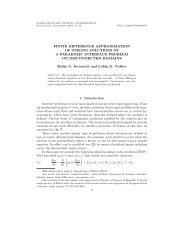
Fine Type Decomposition of T d−1<br />
(∅, ∅,1234) (∅,4,123) (∅,34,12)<br />
(23,4,1)<br />
v1<br />
(3, 4,12)<br />
(1234, ∅, ∅) (123,4, ∅) (23, 14, ∅) (2,134, ∅) (∅,1234, ∅)<br />
-1<br />
-1 0 1 2 3 4 5<br />
v3<br />
(3,14,2)<br />
(∅,134,2)<br />
. . . induced by max-tropical hyperplane arrangement A(V )<br />
v2
duality between min and max:<br />
Recall: Max-<strong>Tropical</strong> Hyperplanes<br />
max(−x, −y) = −min(x, y)<br />
Remark<br />
T is min-tropical hypersurface ⇔ −T is max-tropical hypersurface<br />
−α α<br />
min/max
Main Theorem of <strong>Tropical</strong> Convexity<br />
Theorem (Develin & Sturmfels 2004)<br />
The min-tropical polytope tconv(V ) is the union of the bounded<br />
closed cells of the max-tropical hyperplane arrangement A(V ).<br />
4<br />
3<br />
2<br />
1<br />
0<br />
v4<br />
w6<br />
w1<br />
w5<br />
v1<br />
-1<br />
-1 0 1 2 3 4 5<br />
w2<br />
v3<br />
w4<br />
w3<br />
v2<br />
4<br />
3<br />
2<br />
1<br />
0<br />
(3, ∅,124)<br />
v4<br />
(34, ∅, 12)<br />
(234, ∅,1)<br />
(∅, ∅, 1234) (∅,4,123) (∅, 34, 12)<br />
(23,4,1)<br />
v1<br />
(3,4, 12)<br />
(1234, ∅, ∅) (123,4, ∅) (23,14, ∅) (2,134, ∅) (∅,1234, ∅)<br />
-1<br />
-1 0 1 2 3 4 5<br />
v3<br />
(3,14,2)<br />
(∅,134,2)<br />
v2
tconv{v1, . . .,vn} ⊂ T d−1 dual to regular<br />
subdivision of ∆n−1 × ∆d−1 defined by<br />
lifting ei × ej to height vij<br />
general position ←→ triangulation<br />
extra feature: exchanging the factors <br />
tconv(rows) ∼ = tconv(columns)<br />
Products of Simplices<br />
{ab, ca}<br />
∆1 × ∆2<br />
cb<br />
bb<br />
aa ba<br />
tconv(2 points in T 2 )
tconv{v1, . . .,vn} ⊂ T d−1 dual to regular<br />
subdivision of ∆n−1 × ∆d−1 defined by<br />
lifting ei × ej to height vij<br />
general position ←→ triangulation<br />
extra feature: exchanging the factors <br />
tconv(rows) ∼ = tconv(columns)<br />
recall: regular subdivision<br />
Products of Simplices<br />
{ab, ca}<br />
∆1 × ∆2<br />
cb<br />
bb<br />
aa ba<br />
tconv(2 points in T 2 )
P, Q : polytopes in R d<br />
P + Q = {p + q: p ∈ P, q ∈ Q} Minkowski sum<br />
Mixed Subdivisions<br />
Minkowski cell of P + Q = full-dimensional subpolytope<br />
which is Minkowski sum of subpolytopes of P and Q<br />
Definition<br />
Polytopal subdivision of P + Q into Minkowski cells is mixed if for<br />
any two of its cells P ′ + Q ′ and P ′′ + Q ′′ the intersections P ′ ∩ P ′′<br />
and Q ′ ∩ Q ′′ both are faces.<br />
can be generalized to finitely many summands<br />
fine = cannot be refined (as a mixed subdivision!)
fine mixed subdivision of dilated simplex<br />
∆2 + ∆2 + ∆2 + ∆2 = 4∆2<br />
Example With 4 Summands
e1, e2, . . .,en : affine basis of R n−1<br />
φk : R d → R n−1 × R d embedding p ↦→ (ek, p)<br />
Cayley embedding of P1, P2, . . .,Pn :<br />
C(P1, P2, . . .,Pn) = conv<br />
Cayley Trick, General Form<br />
n<br />
φi(Pi).<br />
Theorem (Sturmfels 1994; Huber, Rambau & Santos 2000)<br />
1 For any polyhedral subdivision of C(P1, P2, . . .,Pn) the<br />
intersection of its cells with { 1 <br />
n ei} × Rd <br />
yields a mixed<br />
Pi.<br />
subdivision of 1<br />
n<br />
2 This correspondence is a poset isomorphism from the<br />
subdivisions of C(P1, P2, . . .,Pn) to the mixed subdivisions of<br />
Pi. Further, the coherent mixed subdivisions are bijectively<br />
mapped to the regular subdivisions.<br />
i=1
Cayley Trick for Products of Simplices<br />
consider P1 = P2 = · · · = Pn = ∆d−1 = conv{e1, e2, . . .,ed}<br />
C(∆d−1, ∆d−1, . . .,∆d−1 )<br />
<br />
n<br />
∼ = ∆n−1 × ∆d−1<br />
Corollary<br />
1 For any polyhedral subdivision of ∆n−1 × ∆d−1 the<br />
intersection of its cells with { 1 <br />
ei} × Rd yields a mixed<br />
subdivision of 1<br />
n<br />
· (n∆d−1).<br />
2 This correspondence is a poset isomorphism from the<br />
subdivisions of ∆n−1 × ∆d−1 to the mixed subdivisions of<br />
n∆d−1. Further, the coherent mixed subdivisions are<br />
bijectively mapped to the regular subdivisions.<br />
n
4<br />
3<br />
2<br />
1<br />
0<br />
(1,0,3)<br />
(2,0,2)<br />
(3,0,1)<br />
(0,0,4) (0,1,3) (0,2,2)<br />
(2,1,1)<br />
(1,1,2)<br />
(1,2,1)<br />
(0,3,1)<br />
(4,0,0) (3,1,0) (2,2,0) (1,3,0) (0,4,0)<br />
-1<br />
-1 0 1 2 3 4 5<br />
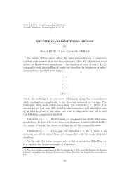
Back to Standard Example<br />
400<br />
fine types coarse types<br />
sum columns of type matrix ∼ replace sets by their cardinality<br />
coarse types of maximal cells = vertex coordinates of mixed<br />
subdivision<br />
301<br />
202<br />
310<br />
103<br />
211<br />
004<br />
112<br />
220<br />
013<br />
121<br />
022<br />
130<br />
031<br />
040
4<br />
3<br />
2<br />
1<br />
0<br />
(1,0,3)<br />
(2,0,2)<br />
(3,0,1)<br />
(0,0,4) (0,1,3) (0,2,2)<br />
(2,1,1)<br />
(1,1,2)<br />
(1,2,1)<br />
(0,3,1)<br />
(4,0,0) (3,1,0) (2,2,0) (1,3,0) (0,4,0)<br />
-1<br />
-1 0 1 2 3 4 5<br />
Back to Standard Example<br />
400<br />
fine types coarse types<br />
sum columns of type matrix ∼ replace sets by their cardinality<br />
coarse types of maximal cells = vertex coordinates of mixed<br />
subdivision<br />
301<br />
202<br />
310<br />
103<br />
211<br />
004<br />
112<br />
220<br />
013<br />
121<br />
022<br />
130<br />
031<br />
040
A <strong>Tropical</strong> Hypersurface<br />
point vi ∈ T d−1 = apex of unique max-tropical hyperplane<br />
H max (vi)<br />
homogeneous linear form hi ∈ C{{z}}[x1, xx, . . .,xd];<br />
h := h1 · h2 · · ·hn<br />
Proposition<br />
The tropical hypersurface defined by trop max (h) is the union of<br />
the max-tropical hyperplanes in A.<br />
Corollary<br />
Let p ∈ T d−1 \ A be a generic point. Then its coarse type tA(p)<br />
equals the exponent of the monomial in h which defines the unique<br />
facet of P(trop max (h)) above p.
Conclusion II<br />
n points in T d−1 ↔ arrangement of n tropical hyperplanes<br />
in T d−1<br />
tropical polytope = union of bounded cells<br />
coarse and fine types<br />
regular subdivision of ∆n−1 × ∆d−1<br />
mixed subdivision of n∆d−1
Conclusion II<br />
n points in T d−1 ↔ arrangement of n tropical hyperplanes<br />
in T d−1<br />
tropical polytope = union of bounded cells<br />
coarse and fine types<br />
regular subdivision of ∆n−1 × ∆d−1<br />
mixed subdivision of n∆d−1
Conclusion II<br />
n points in T d−1 ↔ arrangement of n tropical hyperplanes<br />
in T d−1<br />
tropical polytope = union of bounded cells<br />
coarse and fine types<br />
regular subdivision of ∆n−1 × ∆d−1<br />
mixed subdivision of n∆d−1
Conclusion II<br />
n points in T d−1 ↔ arrangement of n tropical hyperplanes<br />
in T d−1<br />
tropical polytope = union of bounded cells<br />
coarse and fine types<br />
regular subdivision of ∆n−1 × ∆d−1<br />
mixed subdivision of n∆d−1
Conclusion II<br />
n points in T d−1 ↔ arrangement of n tropical hyperplanes<br />
in T d−1<br />
tropical polytope = union of bounded cells<br />
coarse and fine types<br />
regular subdivision of ∆n−1 × ∆d−1<br />
mixed subdivision of n∆d−1
The Coarse Type Ideal<br />
Definition<br />
Let A = A(V ) be an arrangement on n tropical hyperplanes in<br />
T d−1 . The coarse type ideal of A is the monomial ideal<br />
I t(A) = 〈x t(p) : p ∈ T d−1 〉 ⊂ K[x1, . . .,xd]<br />
where x t(p) = x t(p)1<br />
1 x t(p)2<br />
2 · · ·x t(p)d<br />
d .<br />
similar construction for (oriented) matroids<br />
[Novik, Postnikov & Sturmfels 2002]
Powers of the Maximal Ideal<br />
Proposition<br />
If A = A(V ) is sufficiently generic the coarse cotype ideal is<br />
4<br />
3<br />
2<br />
1<br />
0<br />
I t(A) = 〈x1, x2, . . .,xn〉 d .<br />
(1,0,3)<br />
(2,0,2)<br />
(3,0,1)<br />
(0,0,4) (0,1,3) (0,2,2)<br />
(2,1,1)<br />
(1, 1,2)<br />
(1,2,1)<br />
(0,3, 1)<br />
(4,0,0) (3,1,0) (2,2,0) (1,3, 0) (0,4,0)<br />
-1<br />
-1 0 1 2 3 4 5
Resolutions via Coarse <strong>Tropical</strong> Convexity<br />
Theorem (Dochtermann, Sanyal & J. 2009+)<br />
Let A be an arrangement of n tropical hyperplanes in T d−1 . The<br />
colabeled complex CA supports a minimal cocellular resolution of<br />
the coarse type ideal I t(A).<br />
Eliahou-Kervaire resolution of 〈x1, x2, . . .,xn〉 d in the<br />
sufficiently generic case
Minimal Free Resolutions<br />
S = K[x1, . . .,xd] polynomial ring with Z d -grading<br />
deg x a = a<br />
free Z d -graded resolution F• of monomial ideal I ⊆ S is<br />
exact (algebraic) complex of Z d -graded S-modules:<br />
F• : · · · φk+1<br />
−→ Fk<br />
φk<br />
−→ · · · φ2<br />
−→ F1<br />
φ1<br />
−→ F0 → 0<br />
Fi ∼ = <br />
a∈Z d S(−a)βi,a free Z d -graded S-modules<br />
maps φi homogeneous<br />
F0 = S and img φ1 = I<br />
i-th syzygy module img φi+1 ⊂ Fi<br />
resolution minimal if βi,a = dimK Tor S i (I, K)a<br />
fine graded Betti numbers
P polyhedral complex<br />
(Co-)Cellular Resolutions I<br />
Z d -labeling of cells with tH = lcm {tG : for G ⊂ H a face}<br />
free modules<br />
Fi =<br />
<br />
H∈P, dim H=i+1<br />
S(−tH)<br />
differentials φi : Fi → Fi−1 given on generators by<br />
φi(H) =<br />
<br />
dim G=dim H−1<br />
ǫ(H, G)x tH−tG G<br />
P≤b = subcomplex of P given by cells H ∈ P with tH ≤ b<br />
for some b ∈ Z d<br />
b-graded component of F P • = cellular chain complex of P≤b
(Co-)Cellular Resolutions II<br />
Proposition<br />
If for every b ∈ Z d the subcomplex P≤b is acyclic over K, then F P •<br />
is a free resolution of the ideal I generated by all monomials<br />
corresponding to the vertex labels of P. Moreover, if tF = tG for<br />
all cells F ⊃ G then the cellular resolution is minimal.<br />
cellular: tH = lcm {tG : for G ⊂ H a face}<br />
cocellular: t H = lcm {tG : for G ⊃ H a face}<br />
reverse arrows: F • P<br />
[Bayer & Sturmfels 1998] [Miller 1998]
201 111 021<br />
300 210 030<br />
chain complex<br />
with img φ1 = I<br />
003 ideal<br />
012<br />
An Example<br />
I = 〈x 3 1, x 2 1x2, x 3 2, x 2 1x3,<br />
x1x2x3, x 2 2x3, x2x 2 3, x 3 3〉<br />
lcm condition <br />
labels for all cells<br />
f(P) = (8, 11, 4)<br />
check condition for each<br />
b ∈ Z d<br />
e.g., b = (2,2,2)<br />
minimal resolution<br />
F P 4 φ3 11<br />
• : 0 → S −→ S φ2 8<br />
−→ S φ1<br />
−→ S → 0
Proposition<br />
Each tropically convex set is contractible.<br />
Proof.<br />
distance of two points p, q ∈ T d−1 :<br />
Digression: <strong>Tropical</strong> Convexity<br />
dist(p, q) := max<br />
1≤i
Proposition<br />
Each tropically convex set is contractible.<br />
Proof.<br />
distance of two points p, q ∈ T d−1 :<br />
Digression: <strong>Tropical</strong> Convexity<br />
dist(p, q) := max<br />
1≤i
Proposition<br />
Each tropically convex set is contractible.<br />
Proof.<br />
distance of two points p, q ∈ T d−1 :<br />
Digression: <strong>Tropical</strong> Convexity<br />
dist(p, q) := max<br />
1≤i
Proposition<br />
Each tropically convex set is contractible.<br />
Proof.<br />
distance of two points p, q ∈ T d−1 :<br />
Digression: <strong>Tropical</strong> Convexity<br />
dist(p, q) := max<br />
1≤i
A = A(V ): max-tropical hyperplane arrangement in T d−1<br />
Key Observation<br />
Proposition<br />
For p, q ∈ T d−1 let r ∈ tconv max {p, q} be an arbitrary point on the<br />
max-tropical line segment between p and q. Then for arbitrary<br />
k ∈ [d]:<br />
tA(r)k ≤ max{tA(p)k,tA(q)k}<br />
Corollary<br />
For arbitrary b ∈ Nd :<br />
<br />
(CA)≤b := p ∈ T d−1 <br />
: tA(p) ≤ b = {C ∈ CA : tA(C) ≤ b}<br />
max-tropically convex and hence contractible.
n = d = 3,<br />
⎛ ⎞<br />
0 1 0<br />
V = ⎝0<br />
1 1⎠<br />
,<br />
0 0 1<br />
b = (2, 2, 2)<br />
2<br />
1<br />
0<br />
(0,0,3) (0,1,2)<br />
v3<br />
(2,0,1) (1,1,1)<br />
-1<br />
-1 0 1 2<br />
v2<br />
v1<br />
(0,2,1)<br />
(3,0,0) (2,1,0) (0,3,0)<br />
Example
A : arrangement of n tropical hyperplanes in T d−1<br />
ΣA : associated mixed subdivision of n∆d−1<br />
Theorem (Dochtermann, Sanyal & J. 2009+)<br />
Main Result, Revisited<br />
The colabeled complex CA supports a minimal cocellular resolution<br />
of the coarse type ideal I t(A).<br />
Corollary<br />
The labeled polyhedral complex ΣA supports a minimal cellular<br />
resolution of the coarse type ideal I t(A).
4<br />
3<br />
2<br />
1<br />
0<br />
(1,0,3)<br />
(2,0,2)<br />
(3,0,1)<br />
(0,0,4) (0,1,3) (0,2,2)<br />
(2,1,1)<br />
(1,1,2)<br />
(1,2,1)<br />
(0,3,1)<br />
(4,0,0) (3,1,0) (2,2,0) (1,3,0) (0,4,0)<br />
-1<br />
-1 0 1 2 3 4 5<br />
A Sufficiently Generic Example<br />
400<br />
301<br />
202<br />
310<br />
I t(A) = 〈x1, x2, x3, x4〉 3<br />
103<br />
211<br />
0 → S 10 → S 24 → S 15 → S → 0<br />
4<br />
004<br />
112<br />
220<br />
013<br />
3<br />
121<br />
022<br />
130<br />
031<br />
1 2<br />
040
2<br />
1<br />
0<br />
v3<br />
-1<br />
-1 0 1 2<br />
003<br />
3<br />
Ideal Generated by Non-generic Points<br />
012<br />
v2<br />
v1<br />
201 111 021<br />
300 210 030<br />
2<br />
1<br />
2<br />
1<br />
0<br />
(0,0,3) (0,1,2)<br />
v3<br />
(2,0,1) (1,1,1)<br />
-1<br />
-1 0 1 2<br />
v2<br />
v1<br />
(0,2,1)<br />
(3,0,0) (2,1,0) (0,3,0)<br />
I = 〈x 3 1, x 2 1x2, x 3 2, x 2 1x3,<br />
x1x2x3, x 2 2x3, x2x 2 3, x 3 3〉<br />
0 → S 4 → S 11 → S 8 → S → 0
Conclusion and Remarks III<br />
tropical hypersurfaces<br />
general tropical varieties defined as subfan of Gröbner fan<br />
[Sturmfels]<br />
tropical curves, coordinate-free approach [Mikhalkin]<br />
tropical convexity<br />
max-plus linear algebra optimization<br />
exterior descriptions<br />
tropical Grassmannians<br />
(co-)cellular resolutions of coarse cotype ideals<br />
goal: characterize these ideals