TH`ESE présentée pour obtenir le grade de DOCTEUR Domaine ...

Titre : CALCUL DENERTIEN
GUO-NIU HAN
TH ÈSE
présentée pour obtenir
le grade de DOCTEUR
Domaine : MATH ÉMATIQUE
Soutenue le 17 janvier 1992 devant la Commission d’Examen :
MM. D. FOATA, Président du Jury,
J.-P. JOUANOLOU, Rapporteur interne,
A. LASCOUX, Rapporteur externe,
J. D ÉSARMÉNIEN,
M. MIGNOTTE.
1991 476/TS-29

UNIVERSITÉ LOUIS PASTEUR
Département de Mathématique
INSTITUT DE RECHERCHE MATHÉMATIQUE AVANCÉE
Unité associée au C.N.R.S. 001
STRASBOURG
TH ÈSE
présentée pour obtenir le grade de
DOCTEUR
par
GUO-NIU HAN
A.M.S. Subject Classification (1980) 05A15 05A17 33A15 33A75
Mots clefs : Statistiques euler-mahoniennes, nombre d’inversions, indice
majeur, permutations, mots, réarrangements, commutation,
tableaux de Young, nombres de Kostka, nombres de
Genocchi, q-analogues.
Titre : CALCUL DENERTIEN
Soutenue le 17 janvier 1992 devant la Commission d’Examen :
MM. D. FOATA, Président du Jury,
J.-P. JOUANOLOU, Rapporteur interne,
A. LASCOUX, Rapporteur externe,
J. D ÉSARMÉNIEN,
M. MIGNOTTE.

TABLE DES MATI ÈRES
Remerciements . . . . . . . . . . . . . . . . . . . . . . . . . . . . . . . . . . . . . . . . . . . . . 3
CHAPITRE 0. — Introduction . . . . . . . . . . . . . . . . . . . . . . . . . . . . . . . . . 5
CHAPITRE 1. — La statistique de Denert . . . . . . . . . . . . . . . . . . . . . . . 9
PARTIE 1.1. — Distribution Euler-mahonienne : une correspondance
. . . . . . . . . . . . . . . . . . . . . . . . . . . . . . . . . . . . . . . . . . . . . 11
PARTIE 1.2. — Une nouvelle bijection pour la statistique de
Denert . . . . . . . . . . . . . . . . . . . . . . . . . . . . . . . . . . . . . . . . . . . . . 17
PARTIE 1.3. — La troisième transformation fondamentale . . . . . 23
CHAPITRE 2. — Statistique sur les tableaux de Young . . . . . . . . . . . 73
PARTIE 2.1. — Croissance des polynômes de Kostka . . . . . . . . . 75
PARTIE 2.2. — Polynômes de Kostka-Foulkes : une étude statistique
. . . . . . . . . . . . . . . . . . . . . . . . . . . . . . . . . . . . . . . . . . . . . . 81
CHAPITRE 3. — Symétries trivariées sur les nombres de Genocchi . 103
Index . . . . . . . . . . . . . . . . . . . . . . . . . . . . . . . . . . . . . . . . . . . . . . . . . . . . . . 119

REMERCIEMENTS
Je tiens d’abord à exprimer toute ma reconnaissance à M. Dominique
FOATA sous la direction et avec l’aide duquel ce travail a été effectué. Ses
conseils judicieux et sa grande expérience tant sur le plan mathématique
que sur le plan humain ainsi que son allant permanent et sa disponibilité,
m’ont été très profitables depuis mon arrivée à Strasbourg.
Je ne saurais oublier M. A. LASCOUX pour son étroite collaboration
de tous les instants ; il m’a fait bénéficier de sa grande expérience en
mathématique et m’a soutenu de façon indéfectible avec une extrême gentillesse
et m’a donné beaucoup de courage en face de toutes les difficultés
rencontrées durant mes séjours à Ivry. Qu’il trouve ici l’expression de toute
ma gratitude.
Je remercie vivement M. J.-P. JOUANOLOU, qui a fidèlement écouté
mes exposés au séminaire, et a bien voulu rapporter sur mes travaux. Je
remercie également MM. J. DÉSARMÉNIEN et M. MIGNOTTE qui m’ont fait
le grand plaisir de juger ce travail en participant au jury.
Mes remerciements vont aussi à M. M.-P. SCH ÜTZENBERGER qui m’a
consacré beaucoup de son temps précieux pour de nombreuses discussions
sur les mathématiques et l’informatique qui m’ont beaucoup aidé.
Je tiens également à remercier mes collègues D. DUMONT et J. ZENG
sans l’aide desquels ce travail n’aurait pu être mené à bien. Enfin Raymond
SEROUL a eu la gentillesse de me faire bénéficier de tout son savoir-faire
en typographie informatique.

CHAPITRE 0
INTRODUCTION
Le titre initial qui avait été donné à cette thèse était “ Études statistiques
sur le groupe symétrique et les tableaux de Young.” En effet, le but
de ce travail était d’étudier les propriétés d’une large classe de statistiques
sur ces dernières structures. Dans la rédaction finale, le chapitre 1 a pris
une place tellement prépondérante qu’il a fourni en fait le titre de la thèse.
On sait depuis MACMAHON [MacM] que les statistiques indice majeur
(“maj”) et nombre d’inversions (“inv”) ont même distribution non
seulement sur le groupe symétrique, mais aussi sur toute classe de
réarrangements d’un mot (avec éventuellement répétition d’une même lettre).
Il en est de même des statistiques nombre d’excédances (“exc”) et
nombre de descentes (“des”). Le polynôme générateur de “des” (donc
de “exc”) sur le groupe symétrique est le polynôme eulérien [F-S] et
le polynôme générateur du couple (des, maj) est le q-analogue de ce
polynôme. On dit encore que ce couple est euler-mahonien. La question
naturelle qui se posait était de trouver la statistique qu’il fallait associer
à “exc” pour que la paire ainsi constituée soit aussi euler-mahonienne.
On doit à DENERT [Den] d’avoir imaginé la définition de cette statistique,
appelée “den” par la suite, dans un contexte tout à fait différent,
celui des fonctions zêta attachées aux structures d’ordre de certaines
algèbres simples.
Le fait que le couple (exc, den) est euler-mahonien a tout d’abord
été démontré par FOATA et ZEILBERGER [F-Z]. Une première question
naturelle qui se posait était d’établir ce résultat combinatoirement, c’està-dire
sachant que la paire classique (des,maj) est euler-mahonienne, de
construire une bijection de Sn sur lui-même qui envoie la paire (des,maj)
sur la paire (exc,den).

6 Guo-Niu HAN
Nous avons donné la construction de deux telles bijections, décrites
dans deux notes aux Compte-Rendus, reproduites ici comme parties 1.1
et 1.2.
La seconde question naturelle qui se posait était d’étendre le résultat
de FOATA et ZEILBERGER, valable pour le seul groupe symétrique, au
cas des classes de réarrangements de mots quelconques. Une première
difficulté était de prolonger la définition de “den” elle-même au cas des
mots arbitraires. Nous avons pu le faire à partir d’une formule équivalente
établie par ces auteurs.
Le problème majeur à résoudre ensuite était de construire une bijection
d’une classe de réarrangements sur elle-même qui envoie le couple (des,
maj) sur (exc, den). Pour ce faire, nous avons dû faire tout d’abord une
étude systématique des statistiques sur le groupe symétrique et le monoïde
libre ordonné. Il a fallu reprendre ensuite l’étude de l’algèbre des circuits
telle qu’elle avait été développée dans CARTIER-FOATA [C-F]. La loi de
transposition des circuits devient ici beaucoup plus complexe, mais conduit
tout naturellement en utilisant ce que nous appellons h-multiplication vers
la construction explicite de cette bijection.
Le résultat principal de cette partie est consigné dans les théorèmes
10.4.1 et 10.5.8. La bijection définie sur le monoïde libre ordonné qui envoie
la paire (exc, den) sur (des, maj) est appelée “troisième transformation
fondamentale,” faisant suite aux deux transformations fondamentales qui
envoyaient “exc” sur “des”, et “maj” sur “inv,” respectivement. On peut
ainsi considérer cette nouvelle transformation comme le q-analogue de la
première tansformation fondamentale.
Le deuxième chapitre est consacré à une étude combinatoire et analytique
des polynômes de Kostka-Foulkes Kν,θ(q) (ν, θ étant des partitions
et q une variable), définis comme les coefficients de la matrice de passage,
dans l’algèbre des fonctions symétriques, de la base des fonctions de
Schur à celle formée par les fonctions de Hall-Littlewood. On sait d’après
les travaux de LASCOUX et SCHÜTZENGBERGER [L-S] que ces polynômes
sont à coefficients entiers positifs. Ces auteurs ont, en effet, démontré que
Kν,θ(q) était le polynôme générateur de l’ensemble des tableaux de forme
ν et d’évaluation θ par une certaine statistique à valeurs entières appelée
charge.
Nous avons utilisé cette interprétation combinatoire pour étudier les
propriétés de croissance de ces polynômes et répondu ainsi, dans une

Introduction 7
Note aux Compte-Rendus, reproduite comme partie 2.1 ici, à une conjecture
proposée par GUPTA-BRYLINSKI [Gup], à savoir démontré l’inégalité
Kλ,µ(q) ≤ Kλ∪a,µ∪a(q).
Le problème qui reste ouvert est d’étudier la limite limn Kλ∪a n ,µ∪a n(q).
Sous cette forme générale, le problème reste trop complexe. Suivant une
suggestion de LASCOUX, il semble plus fructueux de trouver une expression
simple pour la somme de la série
n≥0 zn Kλ∪an ,µ∪an(q). On conjecture
que cette somme est une fraction rationnelle en q dépendant naturellement
des paramètres λ, µ et a.
Dans ce chapitre, le calcul est explicitement fait dans le cas où a = 1,
q = 1 et µ = 11 . . . 1, c’est-à-dire dans le cas des tableaux de Young de
forme λ. On trouve, en effet, une fraction rationnelle Pλ(1−z)/(1−z) |λ|+1 .
Le calcul nous a amené à introduire des statistiques nouvelles sur les
tableaux de Young et à les étudier pour leur intérêt propre. En particulier,
le numérateur Pλ(z) est en fait la fonction génératrice de l’ensemble des
tableaux de forme λ par la première lettre “pre” et aussi la fonction
génératrice de ce même ensemble par une seconde statistique “deu.” Le
fait inattendu est que la distribution jointe de ces deux statistiques est
symétrique. Ce que nous établissons par la construction d’un algorithme
simple.
Dans le cas où q est quelconque, nous avons obtenu le résultat explicite
suivant
Kt1n(q)zn =
n≥0
charge t q
(1 − zqc )(1 − zqc+1 ) . . . (1 − zqc+m−p ) ·
Ces derniers résultats sont consignés dans la partie 2.2.
Dans le chapitre 3, nous proposons une extension de la théorie
géométrique des nombres de Genocchi introduite par DUMONT. Celui-ci a
démontré que ces nombres définis par G2n = 2(2 2n −1)B2n, où B2n désigne
le nombre de Bernoulli de rang n, comptaient les fonctions excédantes de
l’intervalle {1, 2, . . . , 2n} qui sont surjectives sur {2, 4, . . . , 2n}. DUMONT
et FOATA [D-F] avaient établi une propriété de symétrie trivariée sur
cet ensemble de fonctions. En fait, on peut définir une classe beaucoup
plus importante de statistiques trivariées qui ont aussi cette propriété de
symétrie. Pour toute suite U dont les lettres sont X, Y et Z, on définit des
points U-maximaux, U-fixes, et U-surfixes ; on démontre que le polynôme
générateur de ces statistiques est indépendant de la suite U. De cette

8 Guo-Niu HAN
façon, la symétrie de ce polynôme à trois variables est évidente. On introduit,
enfin, un codage des fonctions excédantes, servant à construire
une involution qui conserve ces statistiques “max” et “fix”, et échange le
nombre de points saillants et le nombre de points surfixes.
BIBLIOGRAPHIE
[C-F] P. CARTIER et D. FOATA. — Problèmes combinatoires de permutations et
réarrangements. — Berlin, Springer-Verlag, 1969 (Lecture Notes in Math., 85).
[Den] M. DENERT. — The genus zeta function of hereditary orders in central simple
algebras over global fields, Math. Comp., t. 54, 1990, p. 449–465.
[D-F] D. DUMONT et D. FOATA. — Une propriété de symétrie des nombres de Genocchi,
Bull. Soc. math. France, t. 104, 1976, p. 433-451.
[F-S] D. FOATA et M.-P. SCHÜTZENBERGER. — Théorie géométrique des polynômes
eulériens. — Berlin, Springer-Verlag, 1970 (Lecture Notes in Math., 138).
[F-Z] D. FOATA et D. ZEILBERGER. — Denert’s Permutation Statistic Is Indeed Euler-
Mahonian, Studies in Appl. Math., t. 83, 1990, p. 31–59.
[Gup] G. GUPTA. — Problem No. 9, in Combinatorics and Algebra [C. GREENE, éd.
1984], p. 310. — Contemporary Mathematics, vol.34.
[L-S] A. LASCOUX et M.-P. SCHÜTZENBERGER. — Le monoïde plaxique, Non-commutative
Structures in Algebra and geometric Combinatorics [A. de Luca, ed.,
Napoli. 1978], p. 129–156. — Roma, Consiglio Nazionale delle Ricerche, 1981
(Quaderni de “La Ricerca Scientifica”, 109).
[MacM] P.A. MACMAHON. — The indices of permutations and the derivation therefrom of
functions of a single variable associated with the permutations of any assemblage
of objects, Amer. J. Math., t. 35, 1913, p. 281–322.

CHAPITRE 1
LA STATISTIQUE DE DENERT
L’étude des statistiques euler-mahoniennes a été remise en faveur
récemment à la suite des travaux de Denert [Den] sur le calcul des fonctions
zêta attachées aux structures d’ordre de certaines algèbres simples. D’un
point de vue proprement combinatoire, on lui doit l’introduction d’une
nouvelle statistique d’ordre sur les permutations, appelée “den” dans tout
le présent travail, et d’avoir conjecturé que la paire (exc, den), où “exc”
est le nombre usuel d’excédances d’une permutation, avait la distribution
euler-mahonienne sur le groupe symétrique.
Le résultat a été démontré tout d’abord par FOATA et ZEILBERGER
[F-Z] et la question naturelle qui se posait était d’établir ce résultat
combinatoirement, c’est-à-dire sachant que la paire classique (des,maj)
est euler-mahonienne, de construire une bijection de Sn sur lui-même qui
envoie la paire (des,maj) sur la paire (exc,den).
Nous avons donné la construction de deux telles bijections, dans deux
notes aux Compte-Rendus, que nous reproduisons dans le présent chapitre
en parties 1.1 et 1.2. La première de ces bijections repose sur une manipulation
des chemins de Motzkin valués ; elle a pour propriété complémentaire
de donner une démonstration directe du fait que le cardinal de l’ensemble
de ces chemins est n! sans passer par l’intermédiaire du groupe symétrique.
La seconde bijection utilise une extension du procédé d’insertion de
RAWLINGS et fournit aussi une démonstration directe du fait que les deux
paires (des, maj) et (exc, den) sont euler-mahoniennes.
A priori, la statistique “den” se prêtait mal aux calculs. Pour la rattacher
aux autres statistiques mahoniennes, comme l’indice majeur “maj”
et le nombre d’inversions “inv,” il a fallu faire une étude globale de
toutes les distributions euler-mahoniennes. L’introduction des invervalles
cycliques permet de trouver le cadre naturel englobant toutes les statistiques
classiques, y comprix “den.”

10 Chap. 1
Cette recherche du bon cadre algébrique nous a conduit à prolonger le
résultat de Foata-Zeilberger, valable sur les seuls groupes symétriques, aux
classes des réarrangements de mots quelconques (avec répétitions). La difficulté
initiale était de trouver d’abord la bonne définition de “den” pour
les mots quelconques, ensuite de construire une bijection d’une classe de
réarragements sur elle-même qui envoie la paire (des, maj) sur (exc, den).
La construction de cette bijection, appelée troisième transformation fondamentale,
est donnée dans la troisième partie de ce chapitre.
On connaissait jusqu’ici deux autres transformations du même type,
valables pour toutes les classes de mots. La première envoyait la statistique
eulérienne “exc” sur “des,” la seconde la statistique mahonienne
“maj” sur “inv” (cf. [Fo1]). Cette troisième transformation envoyant une
statistique bivariée euler-mahonienne sur une autre, donc en particulier
“des” sur “exc,” peut être considérée comme le q-analogue de la première
transformation.
Les techniques d’algèbre non-commutative développées ici, bien que
reprenant les méthodes de commutation partielle introduites dans la construction
de la première transformation, sont d’un emploi plus délicat. La
h-transposition, par exemple, définie sur les bimots, dépend fondamentalement
du contexte des deux bilettres consécutives à permuter.
Nous avons fait figurer à la fin de chaque partie de ce chapitre la
bibliographie propre à cette partie. Les références apparaissant dans cette
introduction renvoient à la bibliographie de la troisième partie.

PARTIE 1.1
DISTRIBUTION EULER-MAHONIENNE :
UNE CORRESPONDANCE ( ∗ )
RÉSUMÉ. — Récemment Foata et Zeilberger ont démontré une conjecture due à
Marleen Denert qui affirmait que deux paires de statistiques sur le groupe des permutations
étaient équidistribuées. Cette Note fournit une démonstration combinatoire de
ce fait.
ABSTRACT. — Recently Foata and Zeilberger have proved a conjecture due to
Marleen Denert that asserted that two pairs of statistics on the permutation group were
equidistributed. The present Note provides a combinatorial proof of this statement.
1. Introduction
On appelle mot sous-excédant d’ordre n tout mot s = s1s2 . . . sn de
longueur n dont les lettres si sont des entiers satisfaisant les inégalités
0 ≤ si ≤ i − 1 pour i = 1, 2, . . . , n. On désigne par SEn l’ensemble de ces
mots. La somme s1 + s2 + · · · + sn est notée tot(s), et la valeur eulérienne
eul(s) d’un mot sous-excédant est définie de la façon suivante : d’abord,
eul(s) := 0, si s est de longueur 1 ; ensuite si s = s1s2 . . . sn avec n ≥ 2 :
eul(s1s2 . . . sn) :=
eul(s1 . . . sn−1), si sn ≤ eul(s1 . . . sn−1) ;
eul(s1 . . . sn−1) + 1, si sn ≥ eul(s1 . . . sn−1) + 1.
Ainsi eul(0, 0, 0, 3) = 1, eul(0, 0, 0, 3, 2) = 2, eul(0, 0, 0, 3, 2, 0, 5, 0, 3) = 3.
On dit qu’une statistique (f, g) a la distribution euler-mahonienne, si f
et g sont définies sur un ensemble fini En de cardinal n! et si leur fonction
génératrice tf(σ) qg(σ) , écrite sous la forme
k≥0 An,k(q)tk , satisfait la
relation de récurrence
(1.1) An,k(q) = [k + 1]qAn−1,k(q) + q k [n − k]qAn−1,k−1(q)
( ∗ ) Note publiée dans C.R. Acad. Sci. Paris, t. 310, Série I, p. 311–314,
1990.

12 Chap. 1 – Part. 1.1
pour 1 ≤ k ≤ n − 1 avec les conditions initiales An,0(q) = 1 et An,k(q) = 0
pour k ≥ n. Dans (1.1) on a posé [k]q = 0 pour k = 0 et (1 − q k )/(1 − q)
pour k ≥ 1 (cf. [Car]).
Pour établir combinatoirement qu’une paire (f, g) définie sur En est
euler-mahonienne, il suffit de construire une bijection Ψ : (π, sn) ↦→ σ de
En−1 × [0, n − 1] sur En ayant les propriétés suivantes :
g(σ) = g(π) + sn;
f(π), si 0 ≤ sn ≤ f(π) ;
f(σ) =
f(π) + 1, si f(π) + 1 ≤ sn ≤ n − 1.
Ainsi, (eul,tot) est euler-mahonienne. En appliquant Ψ itérativement,
on obtient une bijection Φ de SEn sur En satisfaisant les propriétés :
eul(s) = f ◦ Φ(s), tot(s) = g ◦ Φ(s). La bijection inverse Φ−1 est appelé le
codage de En.
L’exemple classique de statistique euler-mahonienne sur le groupe des
permutations Sn est fourni par le couple (des, maj), où des et maj sont
respectivement le nombre de descentes et l’indice majeur (cf. [Car], [D-F],
[Raw], [G-G]). Dans ce cas, la bijection Ψ est aisée à construire. Le mot
sous-excédant Φ −1
maj (σ) = Φ−1 (σ) correspondant à σ s’appelle le majcodage
de σ (cf. [Raw]).
Nous nous proposons dans cette Note de faire une construction analogue
pour la statistique bivariée (exc,den) introduite par Denert ([Den]) dont on
sait qu’elle est déjà euler-mahonienne d’après le récent travail de Foata et
Zeilberger ([F-Z]). La statistique “exc” est simplement le nombre classique
des excédances, défini pour toute permutation σ = σ(1)σ(2) . . . σ(n) par
exc(σ) := #{i : 1 ≤ i ≤ n, σ(i) > i}. La statistique “den” est, elle, définie
par
(1.2)
den σ := #{1 ≤ i < j ≤ n : σ(j) < σ(i) ≤ j}
+#{1 ≤ i < j ≤ n : σ(i) ≤ j < σ(j)}
+#{1 ≤ i < j ≤ n : j < σ(j) < σ(i)}.
Dans cette Note on trouvera donc la construction d’un den-codage Φ −1
den .
2. Chemins de Motzkin
Un chemin de Motzkin coloré (ou simplement chemin) de longueur n
est un chemin polygonal dans le quart plan N × N, allant de (0,0) à (n,0)
dont les pas élémentaires sont de quatre sortes : ↗, −→, ⊲, ↘. De plus,

Distribution Euler-mahonnienne 13
il n’y a jamais de pas ⊲ sur l’axe horizontal. On identifiera un tel chemin
au mot w = x1x2 . . . xn, dit de Motzkin coloré, dont les lettres sont prises
dans l’alphabet {↗, −→, ⊲, ↘}. Pour chaque xr, la hauteur de xr, notée
hr(w), est définie par :
⎧
⎪⎨
#{s < r : xs =↗} − #{s < r : xs =↘},
si xr =↗ ou −→;
(2.1) hr(w) :=
⎪⎩
#{s < r : xs =↗} − #{s < r : xs =↘} − 1,
si xr =↘ ou ⊲.
Une évaluation d’un mot w est une suite t = t1t2 . . . tn tel que 0 ≤ tr ≤
hr(w) pour tout r = 1, 2, . . . , n. Le nombre de montées, noté mon(w), est
defini par : mon w := |w|↗ + |w| ⊲ . De plus, tout couple u = (w, t), où t
est une évaluation de w, est appelé chemin (mot) évalué. L’ensemble des
mots évalués de longueur n est noté Un et le sous-ensemble de ces mots
u = (w, t) tels que mon(u) := mon(w) = k est noté Un,k. Enfin, l’indice
ind(u) de u est defini comme la somme des places des montées et de tous
les tr, c’est-à-dire ind(u) := {r : xr =↗ ou ⊲} + n r=1 tr .
Foata et Zeilberger [F-Z] ont établi une bijection Θ de Sn sur Un,
différente de la bijection classique (cf. [Vie]), ayant la propriété exc(σ) =
mon Θ(σ), den(σ) = ind Θ(σ), pour tout σ ∈ Sn. Le reste de la Note va
être consacré à la construction d’une bijection Φden : SEn → Un ayant
la propriété eul(s) = mon Φden(s), tot(s) = ind Φden(s), et la suite des
bijections
Φmaj Φden Θ
Sn←−−−−−−−SEn
−−−−−−−→ Un←−−−−−−−Sn
(des, maj) (eul, tot) (mon, ind) (exc, den)
fournira la correspondance σ ↦→ σ ′ telle que exc(σ) = des(σ ′ ) et den(σ) =
maj(σ ′ ). Comme déjà signalé précédemment, il nous suffira de construire
une bijection
(2.2)
Ψden : (v, sn) ↦−→ u
Un−1,k × [0, k] + Un−1,k−1 × [k, n − 1] −→ Un,k
satisfaisant ind(u) = ind(v) + sn.

14 Chap. 1 – Part. 1.1
3. La Bijection
Il est commode d’introduire la notion de chemin évalué pointé. Il y en
a de deux sortes :
(3.1)
(3.2)
⊲
Un−1,k := {(u, p) : u ∈ Un−1,k, xp =↘ ou ⊲ };
−−−−−−→
Un−1,k−1 := {(u, p) : u ∈ Un−1,k−1, xp =↘ ou −→ };
Puis, on définit l’indice “ind” pour les chemins évalués pointés. Si
⊲
(u, p) ∈ Un−1,k, on marque tous les pas ↘ ou ⊲ dont le nombre total est
exactement k, et on les numérote 1, 2, . . . , k de droite à gauche. On pose
alors :
ind(u, p) := #{r ≥ p : xr =↘ ou ⊲}.
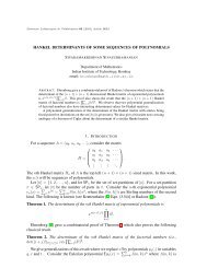
Le chemin inférieur de la figure 1 est un chemin évalué pointé (u, p)
avec comme paramètres : n − 1 = 14, k = 6, p = 5, ind(u, p) = 5. Si
(u, p) ∈ −−−−−−→
Un−1,k−1, on marque tous les pas ↘ et −→ dont le nombre total
est exactement n − k, et on les numérote k, k + 1, . . . , n − 1 de gauche à
droite. De même, on pose
ind(u, p) := (k − 1) + #{r ≤ p : xr =↘ ou −→}.
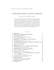
Par exemple, avec n − 1 = 14, k − 1 = 6, p = 5, ind(u, p) = 8, on
obtient le chemin inférieur de la figure 2. Pour construire l’application
Ψden, on distingue deux cas suivant que (v, sn) , avec v = (w, t) =
(x1x2 . . . xn−1, t1t2 . . . tn−1), appartient à Un−1,k × [0, k] ou à Un−1,k−1 ×
[k, n − 1] (cf. (2.2)).
Premier cas. — Supposons (v, sn) ∈ Un−1,k × [0, k]. D’abord si sn = 0,
on définit u = Ψden(v, sn) := (x1x2 . . . xn−1 → , t1t2 . . . tn−10). Par contre,
⊲
si sn = 0, d’après la définition de ind, on sait qu’il existe dans Un−1,k un
chemin évalué pointé unique (v, p) tel que ind(v, p) = sn. On fait alors
correspondre un chemin w ′ = y1y2 . . . yn et une suite t ′ = l1l2 . . . ln de la
façon suivante :
(W1) yr = xr, si r ≤ n − 1 et r = p ;
(W2) yp =−→, si xp =↘ ;
yp =↗,
(W3) yn =↘ ;
si xp = ⊲ ;
(T1) lr = tr, si r ≤ p − 1 ;
(T2) lp = hp(w ′ ) ;
(T3) lr+1 = tr, si p ≤ r ≤ n − 1, et xr =↘ ou −→ ;
lr+1 = tr + 1, si p ≤ r ≤ n − 1, et xr =↗ ou ⊲.

Distribution Euler-mahonnienne 15
r =
t =
1
t1
6
2
t2
3
t3
4
t4
5
p
5
t5
6
t6
7
t7
4 3
t ′ = t1 t2 t3 t4 h5(w ′ ) t5 t6+1 t7 t8+1 t9+1 t10 t11 t12 t13 t14
8
t8
Fig.1
Second cas. — Supposons (v, sn) ∈ Un−1,k−1 × [k, n − 1]. De même,
il existe dans −−−−−−→
Un−1,k−1 un chemin évalué pointé unique (v, p) tel que
ind(v, p) = sn. On fait alors correspondre un chemin w ′ = y1y2 . . . yn
et une suite t ′ = l1l2 . . . ln de la façon suivante :
(W1’) yr = xr, si r ≤ n − 1 et r = p ;
(W2’) yp = ⊲, si xp =↘ ; yp =↗, si xp =−→ ;
(W3’) yn =↘ ;
(T1’) lr = tr, si r ≤ p ;
(T2’) lp+1 = 0 ;
(T3’) lr+1 = tr, si p + 1 ≤ r ≤ n − 1, et xr =↘ ou −→ ;
lr+1 = tr + 1, si p + 1 ≤ r ≤ n − 1, et xr =↗ ou ⊲.
PROPOSITION 3.1. — On a : (w ′ , t ′ ) ∈ Un,k et ind(w ′ , t ′ ) = ind(v) + sn.
On pose alors u = Ψden(v, sn) := (w ′ , t ′ ). L’entier p est dit la place de
changement par rapport à u.
Pour le premier cas, on reprend l’exemple de la figure 1. La place de
changement est p = 5. On a 5 = hp(w ′ ) + 3 et on obtient le chemin
supérieur de la figure 1. Pour le second cas, on reprend l’exemple de la
figure 2, la place de changement étant p = 5. On a 8 = p + 3 et on obtient
le chemin supérieur representé dans la figure 2.
9
t9
10
t10
11
t11
2
12
t12
w
13
t13
1
14
t14
w ′
15

16 Chap. 1 – Part. 1.1
r =
t =
1
t1
7
2
t2
3
t3
4
t4
8
p
5
t5
6
t6
9
7
t7
8
t8
9
t9
10
10
t10
11 12
t ′ = t1 t2 t3 t4 t5 0 t6+1 t7 t8+1 t9+1 t10 t11 t12 t13 t14
Fig.2
PROPOSITION 3.2. — L’application Ψden ainsi construite est inversible.
BIBLIOGRAPHIE
[Car] L. CARLITZ. — q-Bernoulli and Eulerian numbers, Trans. Amer. Math. Soc., t. 76,
1954, p. 332–350.
[Den] M. DENERT. — The genus zeta function of hereditary orders in central simple
algebras over global fields, Math. Comp., t. 54, 1990, p. 449–465.
[D-F] J. DÉSARMÉNIEN et D. FOATA. — Fonctions symétriques et séries hypergéométriques
basiques multivariées, Bull. Soc. Math. France, t. 113, 1985, p. 3–22.
[F-Z] D. FOATA et D. ZEILBERGER. — Denert’s Permutation Statistic Is Indeed Euler-
Mahonian, Studies in Appl. Math., t. 83, 1990, p. 31–59.
[F-S] D. FOATA et M.-P. SCHÜTZENBERGER. — Major Index and Inversion Number of
Permutations, Math. Nachr., t. 83, 1978, p. 143–159.
[G-G] A. GARSIA et I. GESSEL. — Permutation Statistics and Partitions, Adv. in Math.,
t. 31, 1979, p. 288–305.
[Raw] D. RAWLINGS. — Generalized Worpitzki Identites with Applications to Permutation
Enumeration, Europ. J. Comb., t. 2, 1981, p. 67–78.
[Vie] G. VIENNOT. — Une Théorie Combinatoire des Polynômes Orthogonaux Généraux,
Notes conf. Univ. Québec à Montréal, 1984.
11
t11
12
t12
w
13
13
t13
14
14
t14
w ′
15

PARTIE 1.2
UNE NOUVELLE BIJECTION
POUR LA STATISTIQUE DE DENERT ( ∗ )
RÉSUMÉ. — Pour le théorème de Foata-Zeilberger sur les statistiques de Denert, on
a construit dans [Han] une bijection indirecte en passant par les chemins évalués. Dans
cette Note, on trouvera une bijection définie directement sur le groupe des permutations.
ABSTRACT. — A bijection was constructed in [Han] for the Foata-Zeilberger
theorem on Denert’s statistic. This note provides the construction of another bijection
directly defined on the permutation group.
1. Introduction. — Soit σ = σ(1)σ(2) · · · σ(n) une permutation
d’ordre n. Si σ(i) > i, on dit que i est une place excédante pour σ et
σ(i) est une valeur excédante pour σ. Soient Exc(σ) = σ(i1)σ(i2) · · · σ(ik)
le sous-mot des valeurs excédantes et Nexc(σ) = σ(j1)σ(j2) · · · σ(jn−k) le
sous-mot des valeurs non-excédantes. La statistique “exc” est simplement
le nombre des excédances, i.e., la longueur du mot Exc(σ), et la statistique
“den” est définie par (cf. [F-Z], [Den])
den(σ) := Σ{i : σ(i) > i} + inv Exc(σ) + inv Nexc(σ),
où la statistique “inv” est le nombre d’inversion. Par exemple, si
1
σ =
7
2
1
3
5
4
4
5
9
6
2
7
6
8
3
9
,
8
on a den(σ) = 1 + 3 + 5 + inv(759) + inv(142638) = 13.
Comme d’habitude, les statistiques “des” et “maj” sont respectivement
le nombre de descentes et l’indice majeur pour les permutations. On dit
( ∗ ) Note publiée dans C.R. Acad. Sci. Paris, t. 310, Série I, p. 493–496,
1990.

18 Chap. 1 – Part. 1.2
qu’une statistique bivariée (f, g) définie sur le groupe des permutations
d’ordre n a la distribution euler-mahonienne, si (f, g) est équidistribuée
à la statistique bivariée (des, maj). Dans [F-Z], Foata et Zeilberger ont
démontré la conjecture suivante due à Denert :
THÉORÈME 1.1 ([F-Z]). — La statistique bivariée (exc, den) a la distribution
euler-mahonienne.
Dans une note précédente [Han] nous avions démontré combinatoirement
ce résultat en établissant une bijection Φ entre les mots sousexcédants
et les chemins valués. Pour obtenir une bijection définie sur
Sn, il fallait encore prendre le produit de composition de Φ par une bijection
entre Sn et les chemins valués, établi par Foata et Zeilberger [F-Z].
La bijection proposée dans cette note est une bijection directe sur Sn.
Pour établir combinatoirement qu’une paire de statistiques (f, g) définie
sur Sn est euler-mahonienne, il suffit de construire une bijection Ψ :
(σ, s) ↦→ π de Sn−1 × [0, n − 1] sur Sn ayant les propriétés suivantes
(cf. [Car], [Han], [Raw]) :
g(π) = g(σ) + s;
f(σ) , si 0 ≤ s ≤ f(σ) ,
f(π) =
f(σ) + 1 , si f(σ) + 1 ≤ s ≤ n − 1 .
C’est la construction d’une telle bijection Ψ que nous allons décrire ici.
2. La Bijection. — Soit σ ∈ Sn−1. On fait correspondre d’abord une
permutation ν ∈ Sn−1, appelée numérotation de σ, de la façon suivante :
ν(r) :=
# i ≥ r : i ∈ Exc(σ) , si r ∈ Exc(σ) ;
# i ≤ r : i ∈ Nexc(σ) + exc(σ) , si r ∈ Nexc(σ) .
En reprenant l’exemple de la section 1, on peut réprésenter σ et sa
numérotation ν par les trois lignes suivantes :
place − ligne 1 2 3 4 5 6 7 8 9
valeur − ligne 7 1 5 4 9 2 6 3 8
numéro-ligne 2 4 3 7 1 5 8 6 9.
Soit 0 ≤ s ≤ n−1. Si s = 0, on définit Ψ(σ, 0) := σ(1)σ(2) · · · σ(n−1) n.
Si s = 0, on construit la permutation Ψ(σ, s) de la façon suivante :

Une nouvelle bijection 19
[B1].— Dans la valeur-ligne, on souligne σ(i) s’il est une valeur excédante
et si σ(i) ≥ ν −1 (s). L’ensemble de toutes les valeurs soulignées
ν −1 (1), ν −1 (2), · · · , ν −1 (k)
est noté Soul(σ).
[B2].— On remplace les valeurs soulignées de grande à petite en commençant
par n et en sortant la plus petite valeur soulignée p := ν −1 (k),
d’où une suite de remplacement
n = ν −1 (0) ↦→ ν −1 (1) ↦→ ν −1 (2) ↦→ · · · ↦→ ν −1 (k) = p ,
où par convention, ν(n) = 0. Ainsi, on a
(2.1)
p > σ(i) ≥ ν −1 (s) , σ(i) > i = ∅ .
[B3].— On insère p à la place ν −1 (s) qui est appelée la place d’insertion
par rapport à π, et on ajoute n à la fin de la place-ligne.
Autrement dit, la permutation π := Ψ(σ, s) est définie comme suit :
a) π(i) := σ(i) si i < ν −1 (s) et σ(i) /∈ Soul(σ) ;
b) π(i + 1) := σ(i) si i ≥ ν −1 (s) et σ(i) /∈ Soul(σ) ;
c) π(i) := ν −1 (l − 1) si i < ν −1 (s) et σ(i) = ν −1 (l) ∈ Soul(σ) ;
d) π(i + 1) := ν −1 (l − 1) si i ≥ ν −1 (s) et σ(i) = ν −1 (l) ∈ Soul(σ) ;
e) π(ν −1 (s)) = ν −1 (k) .
Dans le tableau de la page suivante, on donne deux exemples pour
illustrer la construction de l’image Ψ(σ, s).
LEMME 2.1 (DUMONT [Dum]). — Soit σ une permutation d’ordre n et
v un entier. On a
DÉMONSTRATION. — En effet,
D’où le lemme.
# i ≥ v > σ(i) = # σ(i) ≥ v > i .
m.g. + # i ≥ v, v ≤ σ(i) = # i ≥ v ,
m.d. + # i ≥ v, v ≤ σ(i) = # σ(i) ≥ v .

20 Chap. 1 – Part. 1.2
[B1]
[B2]
[B3]
(2.2)
(2.3)
s=2 s=7
1 2 3 4 5 6 7 8
9
7 1 5 4 9 2 6 3 8
ν −1 (2) = 7
1 2 3 4 5 6 7 8
9
9 1 5 4 10 2 6 3 8
10 ↦→ 9 ↦→ 7 = p
1 2 3 4 5 6 7 8 9 10
9 1 5 4 10 2 7 6 3 8
1 2 3 4 5 6 7 8
9
7 1 5 4 9 2 6 3 8
ν −1 (7) = 4
1 2 3 4 5 6 7 8
9
9 1 7 4 10 2 6 3 8
10 ↦→ 9 ↦→ 7 ↦→ 5 = p
1 2 3 4 5 6 7 8 9
10
9 1 7 5 4 10 2 6 3 8
Ψ(σ, 2) Ψ(σ, 7)
La construction de l’image Ψ(σ, s).
PROPOSITION 2.2. — Posons π = Ψ(σ, s). On a
den(π) = den(σ) + s ;
exc(σ) , si 0 ≤ s ≤ exc(σ) ,
exc(π) =
exc(σ) + 1 , si exc(σ) + 1 ≤ s ≤ n − 1 .
DÉMONSTRATION. — Comme on le verra, la démonstration de (2.3) est
incluse dans celle de (2.2) ; il nous suffit donc de démontrer la première
partie de la proposition. On distingue deux cas suivant que s ≤ exc(σ) ou
s ≥ exc(σ) + 1.
Premier cas.— Supposons 0 ≤ s ≤ exc(σ). La propriété (2.3) est banale
pour s = 0. Si s ≥ 1 (cf. le premier exemple), on a p = ν−1 (s), d’où la
place ν−1 (s) est non-excédante. Pour tout i < ν−1 (s) (resp. i > ν−1 (s)),
i est une place excédante pour π, si et seulement si i (resp. i − 1) est une
place excédante pour σ. On a donc
(2.4)
(2.5)
(2.6)
Σ i : π(i) > i − Σ i : σ(i) > i = # σ(i) > i ≥ ν −1 (s) ;
inv Exc(π) − inv Exc(σ) = 0 ;
inv Nexc(π) − inv Nexc(σ) = # i ≥ ν −1 (s) > σ(i)
= # σ(i) ≥ ν −1 (s) > i ,

Une nouvelle bijection 21
d’après le lemme précédent. Par définition de “den”, on a
den(π) − den(σ) =# σ(i) > i ≥ ν −1 (s) + # σ(i) ≥ ν −1 (s) > i
=# σ(i) ≥ ν −1 (s), σ(i) > i
=s .
Second cas.— Supposons exc(σ) ≤ s ≤ n − 1 (cf. le deuxième exemple),
on peut vérifier que p > ν −1 (s), d’où la place ν −1 (s) est excédante. De
même, On a
(2.4 ′ ) Σ i : π(i) > i −Σ i : σ(i) > i = # σ(i) > i ≥ ν −1 (s) +ν −1 (s) ;
(2.5 ′ ) inv Exc(π) − inv Exc(σ) = # ν −1 (s) > i, σ(i) > i, σ(i) ≥ p ;
(2.6 ′ ) inv Nexc(π) − inv Nexc(σ) = 0.
D’autre part,
ν −1 (s) = # σ(i) ≤ ν −1 (s), i ≥ σ(i) + # ν −1 (s) ≥ σ(i) > i
= s − exc(σ) + # p > σ(i) > i, ν −1 (s) > i ,
où la première partie de la dernière égalité provient de la définition de la
numérotation ν et la seconde de la relation (2.1). Avec
# σ(i) > i ≥ ν −1 (s) + # ν −1 (s) > i, σ(i) > i, σ(i) ≥ p
+ # p > σ(i) > i, ν −1 (s) > i
= # σ(i) > i ≥ ν −1 (s) + # σ(i) > i, ν −1 (s) > i
= # σ(i) > i
= exc(σ) ,
on a enfin
den(π) − den(σ) =ν −1 (s) + # σ(i) > i ≥ ν −1 (s)
=s .
+ # ν −1 (s) > i, σ(i) > i, σ(i) ≥ p
La propriété (2.1) nous suggère de définir la place grande-fixe d’une
permutation π, comme étant une place j, qui soit une place fixe, ou qui
satisfasse la propriété :
Ej = π(i) : π(i) > i, π(j) > π(i) ≥ j = ∅.

22 Chap. 1 – Part. 1.2
LEMME 2.3. — Soit π = Ψ(σ, s) une permutation d’ordre n. Alors
[G1] La place d’insertion ν −1 (s) est une place grande-fixe ;
[G2] Tout j > ν −1 (s) n’est pas une place grande-fixe.
D ÉMONSTRATION. — Soit j > ν−1 (s). Comme j n’est pas une place
fixe, il suffit de considérer le cas où j est une place excédante. Dans ce
cas, on a j > p (cf. [B2]). En écrivant π(j) = ν −1 (k), on peut vérifier que
ν −1 (k + 1) ∈ Ej. D’où [G2].
PROPOSITION 2.4. — L’application Ψ ainsi construite est inversible.
DÉMONSTRATION. — Soit π une permutation. Notons G(π) l’ensemble
des places grandes-fixes. Ou bien exc(π) = 0 et alors toutes les places sont
grandes-fixes, ou bien exc(π) = 0 ; dans ce cas, on note i l’entier défini
par π(i) = min Exc(π). Il appartient évidemment à G(π). On peut alors
faire l’inverse de la procédure [B∗] en prenant maxG(π) comme la place
d’insertion.
BIBLIOGRAPHIE
[Car] L. CARLITZ. — q-Bernoulli and Eulerian numbers, Trans. Amer. Math. Soc., t. 76,
1954, p. 332–350.
[Den] M. DENERT. — The genus zeta function of hereditary orders in central simple
algebras over global fields, Math. Comp., t. 54, 1990, p. 449–465.
[Dum] D. DUMONT. — Interprétations Combinatoires des nombres de Genocchi, Duke
Math.J., t. 41, 1974, p. 305–317.
[F-Z] D. FOATA et D. ZEILBERGER. — Denert’s Permutation Statistic Is Indeed Euler-
Mahonian, Studies in Appl. Math., t. 83, 1990, p. 31–59.
[Han] G.-N. HAN. — Distribution Euler-mahonienne : une correspondance, C.R. Acad.
Sci. Paris, t. 310, 1990, p. 311–314.
[Raw] D. RAWLINGS. — Generalized Worpitzki Identites with Applications to Permutation
Enumeration, Europ.J.Comb., t. 2, 1981, p. 67–78.

La troisième transformation fondamentale 23
PARTIE 1.3
LA TROISIÈME TRANSFORMATION FONDAMENTALE
1. Introduction et statistiques classiques
Dans cet article, nous nous intéressons tout d’abord aux statistiques
définies sur les ensembles En de cardinal n! Par statistique, nous entendons
des fonctions définies sur En à valeurs dans Z. Les ensembles En sont de
type varié : le groupe symétrique Sn, l’ensemble des mots sous-excédants
SEn = {s = s1s2 · · · sn | 0 ≤ si ≤ i − 1}, l’ensemble des chemins de
Motzkin valués Un (cf. [Vie], [Fla], [Dum]), l’ensemble des bi-tableaux de
Young et ceux des bi-tableaux de Fibonacci [Sta]. Les statistiques classiques
sur Sn et SEn dont nous allons faire plus particulièrement l’étude sont les
suivantes (cf. [Den], [F-Z], [Ha1], [Ha2]) :
DÉFINITION 1.1. — Si F est un ensembles d’entiers, on note #F
son cardinal et F la somme de tous les éléments dans F . Soit σ =
σ1σ2 . . . σn ∈ Sn une permutation. On pose :
(i) inv σ = #{i < j | σi > σj} ;
(ii) des σ = #{i | σi > σi+1} ;
(iii) maj σ = {i | σi > σi+1} ;
(iv) exc σ = #{i | σi > i} ;
les statistiques “inv,” “des,” “maj,” “exc” sont appelées classiquement
nombre d’inversions, nombre de descentes, indice majeur, nombre d’excédances
; si 1 ≤ i ≤ n, on dit que i est une place d’excédance ou une place
de non-excédance pour σ, suivant que l’on a σ(i) > i ou σ(i) ≤ i ; soit
i1 < i2 < · · · < ik la suite croissante des places d’excédance et j1 < j2 <
· · · < jn−k la suite croissante des places de non-excédance pour σ ; on forme
alors les sous-mots : Exc σ = σ(i1) . . . σ(ik) et Nexc σ = σ(j1) . . . σ(jn−k),
l’ensemble des lettres de chacun de ces sous mots étant respectivement
noté : {Exc σ} et {Nexc σ}.

24 Chap. 1 – Part. 1.3
(v) den σ =
i #{i | σi > i} + inv Exc σ + inv Nexc σ.
(vi) La charge de chaque lettre σi est définie comme suit : d’abord la
charge ch(1) de la lettre 1 est zéro ; pour i ≥ 1, la charge ch(i + 1) de
la lettre (i + 1) est égale à ch(i), si (i + 1) est à la gauche de i, et vaut
ch(i) + 1, si (i + 1) est à la droite de i. La charge ch(σ) du tableau t est
alors définie comme la somme de tous les ch(i) : ch(σ) =
i ch(i). (cf.
[Ma1], p. 129, [L-S])
Soit s = s1s2 · · · sn ∈ SEn, on définit les statistiques “eul” et “tot” de
la façon suivante :
(vii) d’abord eul s = 0 si n = 1 ; et récursivement pour n ≥ 2,
eul(s1s2 · · · sn−1), si sn ≤ eul(s1s2 · · · sn−1) ;
eul(s1s2 · · · sn) =
eul(s1s2 · · · sn−1) + 1, sinon ;
(viii) tot s = s1 + s2 + · · · + sn.
EXEMPLE 1.2. — Pour la permutation σ = 71548326, on a inv σ = 15,
des σ = 4, maj σ = 15, exc σ = 3 ; de plus, Exc σ = 758, Nexc σ = 14326,
de sorte que inv Exc σ = 1, inv Nexc σ = 3 et den σ = (1+3+5)+1+3 = 13.
Pour le mot sous-excédant s = 000320503, on a eul s = 3 et tot s = 13.
Parmi ces statistiques, “den” est la plus récente ; on connait donc
moins bien ses propriétés. La première étude la concernant repose sur une
conjecture de Denert [Den], qui a été prouvée par Foata et Zeilberger [F-Z].
Pour ce faire, ils ont utilisé une bijection pour traduire la conjecture dans
l’ensemble Un des chemins de Motzkin et bâti ensuite un calcul algébrique
assez complexe.
Dans deux précédentes notes ([Ha1], [Ha2]), nous avons construit deux
bijections explicites pour démontrer directement la conjecture de Denert.
Ceci nous a amené à découvrir de nouvelles propriétés de la statistique de
Denert et à revoir toute l’étude des statistiques dites euler-mahoniennes.
Le présent article a pour but d’énoncer et de démontrer ces propriétés.
Le corollaire 4.6, par exemple, donne pour la première fois un majcodage
assez simple. Le théorème 5.5 donne une M-bijection qui est à la
fois (des, maj)-codageable et (exc, den)-codageable. Dans le corollaire 7.9,
on construit plusieurs statistiques euler-mahoniennes dont le premier
argument est la statistique eulérienne “exc.”
Nous avons été amenés à définir des intervalles cycliques, permettant
d’avoir une description globale des statistiques mahoniennes “inv,” “maj,”
et “den” et obtenir ainsi une extension naturelle de leurs propriétés
classiques. Ceci est traité dans la section 7.

La troisième transformation fondamentale 25
L’action du groupe diédral sur Sn a fourni des propriétés intéressantes
de symétrie de la statistique bivariée (des, maj) (cf. [FS3]). Comme celleci
a même distribution que (exc, den), il paraissait naturel d’imaginer
les opérations géométriques qu’il fallait définir sur Sn pour obtenir des
propriétés analogues pour (exc, den). Nous avons ainsi été amenés à définir
le ζ-complément et le ζ-retournement d’une permutation et à en étudier
les propriétés. Ces nouvelles propriétés sont décrites dans la section 9.
Denert a introduit une famille de polynômes f η (q), où η est une
partition, pour l’étude des fonctions “genus zeta” [Den]. Lorsque η =
111 . . . 1, ces polynômes sont les polynômes q-eulériens, c’est-à-dire, les
fonctions génératrices de la statistique (des, maj) (ou de (exc, den))
sur les groupes symétriques, ce qui est une conséquence du résultat
établi par Foata et Zeilberger. On pouvait s’attendre à ce que pour une
partition quelconque, les polynômes f η (q) soient les fonctions génératrices
de (des, maj) ou de (exc, den) sur des classes de réarrangements de mots
quelconques (avec répétitions).
Les statistiques “exc,” “des” et “maj” pour les mots quelconques sont
classiques (voir ci-dessous). Il restait à trouver une définition adéquate
pour “den” valable pour les mots quelconques et de construire, pour une
classe de réarrangements d’un mot (quelconque), une bijection de cette
classe sur elle-même qui envoie la paire (des, maj) sur (exc, den). Le but
de la seconde partie de cet article (en fait, toute la section 10) est de donner
la construction d’une telle bijection. Nous l’avons appelée “troisième transformation
fondamentale,” les deux premières transformations fondamentales
(valables pour les mots arbitraires) ayant été construites par Foata
([Fo1]). Il reste encore à vérifier que f η (q) est bien la fonction génératrice
de (exc, den) (donc de (des, maj)) sur une classe de mots correspondant à
la partition η. Nous ne le ferons pas ici, car la définition des polynômes
f η (q) proposée par Denert est compliquée, voire inutilisable. Nous avons
préféré rester dans l’algèbre des réarrangements des mots et donner explicitement
la construction de cette transformation fondamentale.
Plus précisément, soient u un mot quelconque de longueur n. Si a
désigne le réarrangement croissant de ce mot, on notera R(u)(= R(a))
la classe de tous les réarrangements du mot u. De façon classique, on
définit exc u, des u, inv u et maj u par :
exc u = #{i | 1 ≤ i ≤ n, ui > ai},
des u = #{i | 1 ≤ i ≤ n − 1, ui > ui+1},
inv u = #{i < j | ui > uj}, maj u = {i | 1 ≤ i ≤ n − 1, ui > ui+1}.

26 Chap. 1 – Part. 1.3
Pour définir den u, nous avons non seulement besoin de “inv” qui
désigne le nombre d’inversions ordinaires, mais aussi le nombre d’inversions
faibles
imv u = #{i < j | ui ≥ uj}.
Comme pour les permutations ordinaires, on dit que pour le mot u =
u1u2 . . . un, l’entier i est une place d’excédance, ou de non-escédance, si
l’on a ui > ai, ou si l’on a ui ≤ ai. Comme dans la définition 1.1(iv), on
peut former les deux sous-mots Exc u et Nexc u.
DÉFINITION 1.3. — Pour un mot u, on pose
den u =
{i | ui > ai} + imv Exc u + inv Nexc u.
i
On notera que dans cette définition on prend les inversions faibles pour
le sous-mot des places d’excédances et les inversions ordinaires pour le
sous-mot des places de non-excédances.
Par exemple, pour le mot
a
=
u
1 1 1 2 3 3 3 3 3 4 5 5 5 5
3 5 3 3 4 5 1 3 5 1 2 5 3 1
on a exc u = 7, puis Exc u = 3533455 et Nexc u = 1312531. D’où
den u = (1 + 2 + 3 + 4 + 5 + 6 + 9) + imv(3533455) + inv(1312531)
= 30 + 9 + 7 = 46.
Le résultat essentiel de ce mémoire est de donner la construction de
cette troisième transformation fondamentale, c’est-à-dire, la construction
d’une bijection u ↦→ u de R(a) sur lui-même satisfaisant
des u = exc u ; maj u = den u.
La construction d’une transformation ayant ces propriétés entraîne le
théorème suivant.
THÉORÈME 1.4. — Pour tout mot u, les deux paires de statistiques
(des, maj) et (exc, den) sont équidistribuées sur R(u).
Pour la construction de la troisième fondamentale, nous avons repris
les techniques de décomposition des bimots en cycles (voir [Fo1]). Il faut
alors recourir à des transpositions de bilettres successives, dont la règle de
commutation est plus complexe que dans le cas de la construction de la
première transformation fondamentale. Nous terminons cette partie par
une présentation de plusieurs tableaux annexes.
,

La troisième transformation fondamentale 27
2. Codage
Supposons donné pour chaque entier n ≥ 1 un ensemble En de
cardinal n!
DÉFINITION 2.1. — On appelle M-bijection une suite de bijections de
la forme :
En−1 × [0, n − 1]
Ψ
−−−−−→ En
(π, x) ↦−−−−−→ σ
(n ≥ 1). On convient que E0 = ∅. On voit alors que la condition #En = n!
est nécessaire dans cette définition. Plusieurs de ces bijections seront
utilisées et notamment :
(i) La M-bijection canonique sur les ensembles SEn, qui à tout mot
sous-excédant s de longueur n−1 et à tout x ∈ [0, n−1] fait correspondre :
Ψcan(s, x) = sx = s1s2 · · · sn−1x ∈ SEn.
(ii) L’insertion par valeur sur les groupes symétriques Sn, qui à toute
permutation π = π1π2 · · · πn−1 ∈ Sn−1 et à tout x ∈ [0, n − 1], fait
correspondre :
Ψval(π, x) = π1π2 · · · πxnπx+1 · · · πn ∈ Sn.
(iii) L’insertion par position encore sur les groupes symétriques Sn,
définie par :
Ψpos(π, x) = π ′ (x + 1) ∈ Sn,
où π ′ est la permutation sur [n] \ {x + 1} dont la réduction Ω(π ′ ) est
égale à π. (Pour la réduction, cf. [Ha3].) Par exemple, Ψpos(71548326, 3) =
816593274.
(iv) L’insertion cyclique. Si π = π1π2 · · · πn−1 ∈ Sn−1 et x ∈ [0, n − 1],
on décompose π = π ′ π ′′ avec |π ′ | = (longueur du facteur π ′ ) = x et on
pose :
Ψch(π, x) = Ω(π ′′ 0π ′ ).
(v) La somme cyclique. Soient σ une permutation à n lettres sur
[0, n − 1] et r ∈ [1, n] ; on note τ = σ + r la permutation sur [n] définie,
pour tout i ∈ [n], par
τi =
σi + r si σi + r ≤ n ;
σi + r − n si σi + r ≥ n + 1.

28 Chap. 1 – Part. 1.3
La M-bijection Ψcyc est alors définie comme la fonction qui envoie le couple
(π, x), où π = π1π2 · · · πn−1, sur
Ψcyc(π, x) = (π1π2 · · · πn−10) + (x + 1).
Par exemple, Ψcyc(71548326, 3) = (715483260) + 4 = 259837614.
(vi) Dans [Ha1], nous avons construit une M-bijection Ψden sur les
ensembles Un des chemins de Motzkin.
(vii) Nous construisons, dans la section 5, une autre M-bijection, appelée
Ψmix, sur les groupes symétriques.
D ÉFINITION 2.2. — Si Ψ est une M-bijection sur les ensembles En, en
appliquant Ψ −1 itérativement, on obtient une bijection Ψ : En → SEn,
appelée codage. Cette bijection Ψ peut être caractérisée par le diagramme
commutatif suivant :
En−1 × [0, n − 1]
⏐
Ψ×id
SEn−1 × [0, n − 1]
Ψ
−−−−−→ En
⏐
Ψ
Ψcan
−−−−−→ SEn
Par exemple, sur Sn, le codage Ψpos donne le complément de tableau
d’inversion : Ψpos(71548326) = 00114115 ; le tableau d’inversion est
012345678 − 00114115 = 01120452 ; d’où inv(71548326) = 15.
3. Introduction aux statistiques euler-mahoniennes
D ÉFINITION 3.1. — Soient f, g deux statistiques sur En. On dit que f
est eulérienne (resp. g est mahonienne, resp. (f, g) est euler-mahonienne),
s’il existe une M-bijection Ψ(π, x) = σ satisfaisant la condition (i) (resp.
la condition (ii), resp. les conditions (i) et (ii)) suivantes :
(i)
(ii)
f(π), si 0 ≤ x ≤ f(π) ;
f(σ) =
f(π) + 1, si f(π) + 1 ≤ x ≤ n − 1 ;
g(σ) =g(π) + x.
Dans les deux derniers cas, le codage Ψ associé à la M-bijection Ψ est
appelé respectivement g-codage et (f, g)-codage et on a g(σ) = tot(Ψ(σ)).
Notons
σ∈Sn tf(σ) qg(σ) =
k≥0 An,k(q)tk la fonction génératrice de la
statistique euler-mahonienne (f, g). Les polynômes An,k(q) sont appelés

La troisième transformation fondamentale 29
polynômes q-eulériens. Posant An,0(q) = 1 et An,k(q) = 0 pour k ≥ n, on
voit que les conditions (i) et (ii) précédentes impliquent immédiatement
la relation de récurrence de Carlitz (cf. [Car]) :
[C] An,k(q) = [k + 1]qAn−1,k(q) + q k [n − k]qAn−1,k−1(q)
(1 ≤ k ≤ n − 1), où l’on a posé : [ k ]q = 1 + q + · · · + q k−1 pour k ≥ 1 .
Le tableau 1 donne des valeurs de ces polynômes pour n ≤ 5. Le
coefficient de q 4 dans le polynôme A5,1 est égal à 4 ; ceci signifie qu’il
y a exactement quatre permutations 12354, 12453, 13452 et 23451, dont
le nombre de descentes et l’indice majeur sont respectivement 1 et 4.
❍ ❍❍❍
k =
n =
0 1 2 3 4
1 1 0 0 0 0
2 1 q 0 0 0
3 1 2q + 2q 2 q 3 0 0
4 1 3q + 5q 2 + 3q 3 3q 3 + 5q 4 + 3q 5 q 6 0
5 1
4q + 9q 2
+9q 3 + 4q 4
6q 3 + 16q 4
+22q 5 + 16q 6 + 6q 7
Tableau 1
4q 6 + 9q 7
+9q 8 + 4q 9
Supposons associée à tout élément π de En−1 une permutation ρ = ρπ ,
notée encore ρ(π, ∗) sur [0, n − 1]. Une telle permutation sera appelée
une renumérotation. Evidemment, si Ψ est une M-bijection et ρ une
renumérotation, la composition Ψ◦ρ définie par le diagramme commutatif
suivant est aussi une M-bijection.
Ψ ◦ ρ
En−1 × [0, n − 1] −−−−−→ En
(π, x)
⏐
⏐ρ
Ψ
✒
En−1 × [0, n − 1]
(π, ρ π (x))
D ÉFINITION 3.2. — Soient g une statistique mahonienne sur En et
Ψ une M-bijection ; s’il existe une renumérotation ρ telle que Ψ ◦ ρ est
q 10

30 Chap. 1 – Part. 1.3
un g-codage, alors le codage Ψ (ou parfois, la M-bijection Ψ) est dit gcodageable.
Soient (f, g) une statistique euler-mahonienne, le mot (f, g)codageable
est défini de la même façon.
REMARQUE 3.3. — Pour vérifier qu’une statistique g est mahonienne,
il suffit de construire une bijection g-codageable. Si g est mahonienne
et Ψ est une M-bijection g-codageable, alors il existe une et une seule
renumérotation ρ telle que Ψ ◦ ρ est un g-codage. Pour la statistique eulermahonienne
(f, g), on a la même propriété.
EXEMPLE 3.4
(i) Sur les ensembles SEn, Ψcan est un (eul, tot)-codage.
(ii) Sur les groupes symétriques Sn, la M-bijection Ψval est invcodageable.
Avec la renumérotation ρ(π, x) = (π, n−x−1), la composition
Ψval ◦ ρ est un inv-codage.
(iii) De même, la M-bijection Ψpos est inv-codageable. Avec la renumérotation
ρ(π, x) = (π, n − x − 1), la composition Ψpos ◦ ρ est un
inv-codage.
(iv) Dans la section suivante, on va démontrer que Ψval est (des, maj)codageable
(cf., par exemple, [Raw]), et que Ψcyc est maj-codageable (cf.
Corollaire 4.6).
(v) Soit σ = σ1σ ′ ∈ Sn, on pose π = σ ′ σ1. Alors, on a ch π = ch σ + 1
si σ1 = 1 et ch π = ch σ + 1 − n si σ1 = 1. D’où ch(Ψchσ) = ch σ + x.
Autrement dit, Ψch est un ch-codage. (cf. [L-S])
(vi) Soit σ ∈ Sn, on définit le nombre de filières de cette permutation
par fil σ = ch n, où ch n est la charge de la lettre n (cf. définition 1.1 (vi)).
Alors, par la bijection qui envoie une permutation σ sur le retournement
de son inverse : σ ↦→ (σ −1 ) r , on vérifie facilement que (fil, ch) est eulermahonienne.
4. Insertion de Rawlings et sa généralisation
En considérant la M-bijection Ψval et les statistiques des et maj, on a
immédiatement :
LEMME 4.1. — Soit π = π1π2 · · · πn−1 ∈ Sn−1 une permutation. Par
convention, on pose π0 = πn = 0. Alors le changement du nombre de
descentes après application de la M-bijection Ψval se calcule par :
des(Ψval(π, x)) − des π =
0, si πx > πx+1 ;
1, si πx < πx+1.

La troisième transformation fondamentale 31
Pour une place x ∈ [0, n − 1], on insère n à cette place pour former
la permutation Ψval(π, x) = · · · πxnπx+1 · · ·. Si πx > πx+1, le nombre
de descentes ne change pas, on met un point au-dessous de cette place ;
sinon, le nombre de descentes augmente d’une unité, on met dans ce cas un
point au-dessus de cette place. On renumérote les points 0, 1, 2, . . . , n − 1
en commençant de droite à gauche pour les points du bas ; puis de
gauche à droite pour ceux du haut. On construit ainsi l’inverse ρ −1 de
la renumérotation ρ.
Par exemple, pour la permutation π = 71548326, on a ρ−1
=
:
0 1 2 3 4 5 6 7 8
5 4 6 3 7 2 1 8 0
ρ −1 (x) • 5 • 6 • 7 • 8
πx < πx+1
π = (0) 7 1 5 4 8 3 2 6 (0)
les places x 0 1 2 3 4 5 6 7 8
πx > πx+1
ρ −1 (x) •4 •3 •2 •1 •0
En examinant les changements de l’indice majeur, on obtient immédiatement
le lemme suivant :
LEMME 4.2. — La M-bijection Ψval est (des, maj)-codageable et a ρ pour
renumérotation (cf., par exemple, [Raw]).
Dans le tableau 2, on a illustré le résultat de ce lemme à l’aide de la
permutation π = 71548326.
x Ψval(π, x) des maj ρ −1 (π, x)
0 9 7 1 5 4 8 3 2 6 5 20 5
1 7 9 1 5 4 8 3 2 6 4 19 4
2 7 1 9 5 4 8 3 2 6 5 21 6
3 7 1 5 9 4 8 3 2 6 4 18 3
4 7 1 5 4 9 8 3 2 6 5 22 7
5 7 1 5 4 8 9 3 2 6 4 17 2
6 7 1 5 4 8 3 9 2 6 4 16 1
7 7 1 5 4 8 3 2 9 6 5 23 8
8 7 1 5 4 8 3 2 6 9 4 15 0
Tableau 2

32 Chap. 1 – Part. 1.3
Cette insertion par valeur peut se généraliser comme suit : soient k un
entier et k une lettre dont la grandeur est comprise entre k − 1 et k (i.e.,
k − 1 < k < k). On définit une M-bijection Ψk, appelée k-insertion, par
[D1] Ψk(π1π2 · · · πn−1, x) = Ω(π1π2 · · · πxkπx+1 · · · πn) ∈ Sn,
où Ω est encore la réduction. Comme la réduction est une opération simple
à faire, on note également Ψk la M-bijection opérant sur les permutations
(non-réduites) de [n − 1] ∪ k.
On a besoin aussi de la notation suivante :
DÉFINITION 4.3. — Soient x, y et z trois nombres réels. On dit que
le triplet (x, y, z) est un triplant, noté x ≥y z, si ou bien x ≥ z avec y
à l’extérieur de l’intervalle [z, x], ou bien x < z avec y à l’intérieur de
]x, z[ ; en d’autres termes, si l’une des conditions suivantes est satisfaite :
y < z ≤ x, z ≤ x < y, ou x < y < z. On utilise les autres écritures
dérivées : x >y z signifie x ≥y z et x = z. On écrit encore x ≤y z, si
x >y z n’est pas vrai.
D ÉFINITION 4.4. — Soit π ∈ Sn [par convention, on pose π0 =
πn+1 = 0] ; on dit qu’il y a une k-descente à la place i, ou que i est
une place de k-descente, si πi > k πi+1, c’est-à-dire si l’une des conditions
suivantes est satisfaite :
πi > πi+1 > k, k > πi > πi+1, πi < k < πi+1.
Le nombre de k-descentes et l’indice k-majeur sont définis par
et
desk(π) = #{i | πi > k πi+1} − 1;
maj k(π) = {i | πi > k πi+1} − n.
LEMME 4.5. — On a en fait desk = des et maj = maj k +n − k + 1.
D ÉMONSTRATION. — Soit π = (π0 = 0)π1π2 · · · πn(πn+1 = 0) une
permutation. On peut décomposer le mot π de façon unique comme suit :
π = p1q1p2q2 · · · prqrpr+1,
où les pi sont des mots dont toutes les lettres sont plus petites que k et
où les qi sont des mots dont toutes les lettres sont plus grandes que k.

La troisième transformation fondamentale 33
q1
x y
p1 p2 p3
Soit x une place de descente ordinaire de π (πx > πx+1). Si πx n’est
pas la dernière lettre d’un facteur qi (1 ≤ i ≤ r), alors x est aussi
une place pour une k-descente ; si πx est la dernière lettre de qi, alors
x est une place de descente ordinaire, mais non de k-descente. Si πy est la
dernière lettre du mot pi (1 ≤ i ≤ r), on voit que y est une place de kdescente,
mais non de descente ordinaire. Ainsi, il y a autant de descentes
que de k-descentes, d’où des +1 = desk +1. De plus, maj π − majk π =
(|p1| + |q1| + · · · + |pr| + |qr|) − (|p1| + · · · + |pr|) = n − k + 1.
Par exemple, pour π = 0 1 2 3 4 5 6 7 8 9
0 7 1 5 4 8 3 2 6 0
est π = 0 · 7 · 1 · 5 · 4 · 8 · 32 · 6 · 0. Les places de descente et de k-descente
sont respectivement {1, 3, 5, 6, 8} et {0, 2, 4, 6, 7}, d’où maj π = 1 + 3 + 5 +
6 + 8 − 8 = 15 et majk π = 0 + 2 + 4 + 6 + 7 − 8 = 11 = maj π − (n − k + 1).
q2
et k = 5, la décomposition
COROLLAIRE 4.6. — La M-bijection Ψcyc est maj-codageable. Avec la
renumérotation ρ(π, x) = (π, n − x − 1), la composition Ψcyc ◦ ρ est un
maj-codage.
D ÉMONSTRATION. — Soit Ψcyc(π, x) = σ, alors i est une place de
descente pour σ, si et seulement si elle est une place de k-descente de π
avec k = n−x (voir le graphe précédent). D’où maj σ = maj k π+(n−1) =
maj π + (n − x − 1).
On a, pour les k-descentes, les mêmes résultats que pour les descentes
ordinaires :
LEMME 4.7. — Le changement du nombre de descentes après application
de la M-bijection Ψk se calcule par :
0, si πx > k
πx+1 ;
des(Ψk(π, x)) − des π =
1, si πx < k
πx+1.
On insère k à la place x ∈ [0, n − 1] pour former la permutation
Ψk(π, x) = · · · πxkπx+1 · · ·. Si l’on a πx > k πx+1, le nombre de descentes
k

34 Chap. 1 – Part. 1.3
ne change pas ; on met alors un point au-dessous de cette place ; sinon, le
nombre de descentes augmente d’une unité ; on met, dans ce cas, un point
au-dessus de cette place. On renumérote les points 0, 1, 2, · · · , n − 1 en
commençant de droite à gauche pour les points en bas ; puis de gauche à
droite pour ceux du haut. On construit ainsi l’inverse de la renumérotation
associée. On la notera ρ −1
k .
Par exemple, si on prend k = 5 et π = 71548326, on a ρ −1
k
:
0 1 2 3 4 5 6 7 8
4 5 3 6 2 7 1 0 8
ρ −1
k (x) •5 •6 •7 •8 πx < 5
πx+1
π = (0) 7 1 5 4 8 3 2 6 (0)
les places x 0 1 2 3 4 5 6 7 8
πx > 5 πx+1
ρ −1
k (x) •4 •3 •2 •1 •0
D’après les deux lemmes précédents, en examinant les changements de
l’indice majeur, on peut vérifier le théorème suivant :
TH ÉORÈME 4.8. — La M-bijection Ψk est (des, maj)-codageable et a
pour renumérotation ρk.
On prend la permutation π = 71548326 et k = 5 ; les exemples du
tableau 3 vérifient ce théorème :
x Ψ5(π, x) des maj ρ −1
k (π, x)
0 5 7 1 5 4 8 3 2 6 4 19 4
1 7 5 1 5 4 8 3 2 6 5 20 5
2 7 1 5 5 4 8 3 2 6 4 18 3
3 7 1 5 5 4 8 3 2 6 5 21 6
4 7 1 5 4 5 8 3 2 6 4 17 2
5 7 1 5 4 8 5 3 2 6 5 22 7
6 7 1 5 4 8 3 5 2 6 4 16 1
7 7 1 5 4 8 3 2 5 6 4 15 0
8 7 1 5 4 8 3 2 6 5 5 23 8
Tableau 3
=

La troisième transformation fondamentale 35
5. Insertion par lettres différentes
Cette section contient le premier résultat principal de cet article.
D’après la section précédente, l’insertion de la lettre k dans une permutation
π fournit une M-bijection Ψk qui est (des, maj)-codageable. Nous allons
construire maintenant une M-bijection (des, maj)-codageable obtenue
par insertion de lettres différentes à des places bien déterminées, insertion
suivie de quelques déplacements de lettres. Le plus remarquable est que
cette nouvelle insertion fait apparaître les quatre statistiques des, maj, exc
et den à la fois. Le résultat général est donné dans les théorèmes 5.4 et 5.5.
D’après la section précédente, à tout nombre k compris entre (k−1) et k
sont associées une M-bijection Ψk et une renumérotation ρk. Par exemple,
si l’on prend la permutation π = 71548326, on peut donner les inverses
des renumérotations ρ −1
k pour k = 9, 8, 7, 5. Celles-ci sont calculées dans
le tableau 4. La dernière ligne fait apparaître une renumérotation ρ −1
mix qui
sera définie plus loin (lemme 5.3).
LEMME 5.1. — Soient k et k + 1 deux entiers consécutifs. Alors, les
deux renumérotations ρ −1
k et ρ −1
k+1ne diffèrent que par une transposition.
Plus précisément, si j = π−1 (k), on a
ρ −1
k
= ρ−1
k+1 ◦ (j − 1, j) .
Soient k < l deux entiers. Si i est une place telle que π(i) < k ou
π(i) > l − 1, alors, pour passer de ρ −1
l à ρ −1
k , on ne permute pas les deux
places (i − 1) et i. Conservons ces mêmes notations dans l’énoncé suivant.
LEMME 5.2. — Le mot ρ −1
l (0, 1, · · · , i − 1) est un réarrangement du mot
ρ −1
k (0, 1, · · · , i − 1).
π = 7 1 5 4 8 3 2 6
places x = 0 1 2 3 4 5 6 7 8
ρ −1
9
ρ −1
8
ρ −1
7
ρ −1
5
(x) = 5 4 6 3 7 2 1 8 0
(x) = 5 4 6 3 2 7 1 8 0
(x) = 4 5 6 3 2 7 1 8 0
(x) = 4 5 3 6 2 7 1 0 8
ρ −1
mix (x) = 4 5 3 6 2 7 1 8 0
Tableau 4
une renumérotation
permettant la construction d’une M-bijection qui soit à la fois
Notre but maintenant est de fabriquer à l’aide des ρ −1
k

36 Chap. 1 – Part. 1.3
(des, maj)- et (exc, den)-codageable. Pour l’exemple ci-dessus on voit que
la nouvelle application définie par
ρ −1
mix (0, 1, 2, 3, 4, 5, 6, 7, 8) = ρ −1
5
= (4, 5, 3, 6, 2, 7, 1, 8, 0)
(0, 1, 2, 3, 4), ρ−1
7
(5, 6), ρ−1 8 (7), ρ−1 9 (8)
est encore une permutation (renumérotation) sur [0, 8]. (Voir les lettres
grasses dans le tableau précédent.)
Quelle est la règle du choix pour les lettres 9, 8, 7 et 5 ? Ici, pour la
première fois, les descentes et les excédances apparaissent dans une même
construction. Soit π ∈ Sn−1 une permutation dont le nombre d’excédances
exc π est égal à h. Les valeurs v = π(i) telles que π(i) > i ont été
appelées valeurs excédantes ; on note Exc π = (v1 < v2 < · · · < vh) la
suite croissante des valeurs excédantes ou, si l’on veut, le réarrangement
croissant du mot Exc π.
Dans l’exemple que nous traitons, Exc(71548326) = 578. Les lettres de
ce mot sont justement les lettres qu’on a choisies pour les insertions dans
le tableau précédent. De façon générale, posons :
[D2] ρ −1
mix (x) =
⎧
⎪⎨
⎪⎩
ρ −1
v1 (x) , si 0 ≤ x < v1 ;
ρ−1 v2 (x) , si v1
· · · · · ·
≤ x < v2 ;
ρ−1 vh (x) , si vh−1 ≤ x < vh ;
ρ −1
n (x) , si vh ≤ x < n.
LEMME 5.3. — L’application ρmix définie ci-dessus est une permutation
sur [0, n − 1].
DÉMONSTRATION. — Soient k < l deux valeurs excédantes consécutives
de la permutation π. On a donc nécessairement : ou bien π(k) < k, ou
bien π(k) > l − 1. Pour démontrer le lemme, il suffit de vérifier que le mot
ρ −1
l (0, 1, · · · , k − 1) est un réarrangement du mot ρ −1
k (0, 1, · · · , k − 1). Ceci
est vrai d’après le lemme 5.2, puisque l’entier k satisfait les conditions de
ce lemme.
On définit la nouvelle M-bijection Ψmix : Sn−1 × [n − 1] → Sn de la
façon suivante : soit Exc π = v1v2 · · · vh la suite croissante des valeurs
excédantes de la permutation π. Par convention, on pose v0 = 0 et
vh+1 = n. Soient x une place et j l’entier tel que vj−1 ≤ x < vj. On
définit (voir [D2] et [D1] ) :
Ψ ′ mix(π, x) = · · · πxvjπx+1 · · · .

La troisième transformation fondamentale 37
Reprenant toujours le même exemple de la permutation π = 71548326,
on a consigné dans la partie gauche du tableau 5 la construction de Ψ ′ .
Il faut faire attention qu’on ne peut pas faire la réduction tout de suite.
En effet, l’application (π, x) ↦→ Ω Ψ ′ mix (π, x) ∈ Sn n’est pas bijective. La
bonne façon est de ne faire la “réduction” que sur les valeurs excédantes.
Plus précisément, dans le mot Ψ ′ mix (π, x), obtenu par une insertion de
la lettre vj, en remplaçant les lettres vj par vj, vj par vj+1, . . ., vh par
vh+1 = n, on trouve une permutation de Sn, notée Ψmix(π, x). La place
x + 1 est appelée place d’insertion de la permutation Ψmix(π, x).
Par exemple, pour π = 71548326 et x = 5, Ψ ′ mix (π, 5) = 715487326,
d’où la suite de remplacement est 8 ←↪ 9, 7 ←↪ 8, 7 ←↪ 7, on a donc
Ψmix(π, 5) = 815497326. La place d’insertion est 6. On a consigné dans la
partie droite du tableau 5 la construction de Ψ.
TH ÉORÈME 5.4. — L’application Ψmix définie ci-dessus est bien une
bijection.
TH ÉORÈME 5.5. — La M-bijection Ψmix est à la fois (des, maj)codageable
et (exc, den)-codageable.
Ces deux théorèmes vont être démontrés dans la section suivante.
x Ψ ′ mix (π, x) des maj ρ−1
mix Ψmix(π, x) exc den µ −1
mix
0 5 7 1 5 4 8 3 2 6 4 19 4 5 8 1 7 4 9 3 2 6 4 17 4
1 7 5 1 5 4 8 3 2 6 5 20 5 8 5 1 7 4 9 3 2 6 4 18 5
2 7 1 5 5 4 8 3 2 6 4 18 3 8 1 5 7 4 9 3 2 6 4 19 6
3 7 1 5 5 4 8 3 2 6 5 21 6 8 1 7 5 4 9 3 2 6 4 20 7
4 7 1 5 4 5 8 3 2 6 4 17 2 8 1 7 4 5 9 3 2 6 3 16 3
5 7 1 5 4 8 7 3 2 6 5 22 7 8 1 5 4 9 7 3 2 6 4 21 8
6 7 1 5 4 8 3 7 2 6 4 16 1 8 1 5 4 9 3 7 2 6 3 15 2
7 7 1 5 4 8 3 2 8 6 5 23 8 7 1 5 4 9 3 2 8 6 3 14 1
8 7 1 5 4 8 3 2 6 9 4 15 0 7 1 5 4 8 3 2 6 9 3 13 0
Tableau 5
6. Démonstrations des théorèmes principaux 5.4 et 5.5
On va d’abord introduire quelques notations.
DÉFINITION 6.1. — Soit n un entier. Pour deux entiers x, y ∈ [n], les

38 Chap. 1 – Part. 1.3
intervalles cycliques sont définis par
[x, y]
[x, y ] =
[1, y] + [x, n]
si x ≤ y,
si x > y ;
[x, y[
[x, y [ =
[1, y[ + [x, n]
si x ≤ y,
si x > y ;
]x, y]
]x, y ] =
si x ≤ y,
]x, y [ =
[1, y] + ]x, n] si x > y ;
]x, y[ si x ≤ y,
[1, y[ + ]x, n] si x > y.
D’après cette définition, on remarque que [x, x] = {x} et [x, x[ =
]x, x] = ]x, x[ = ∅. Soient x, y, z ∈ [n]. En comparant avec la définition
4.3, on voit que x, y, z est un triplant, si et seulement si z ∈ ]y, x].
D ÉFINITION 6.2. — Soit σ ∈ Sn une permutation. Le contenu de la
place i ∈ [n] est le nombre de valeurs excédantes dans l’intervalle cyclique
[i, σi [. Autrement dit :
[D3] ctn i = #{Exc σ} ∩ [i, σi [ .
Une place est dite grande-fixe pour la permutation σ si son contenu est
vide. L’ensemble des places grandes-fixes de σ est noté Gf(σ).
Par exemple, pour la permutation σ = 815497326, on a {Exc σ} =
{5, 7, 8, 9} (les lettres soulignées) et le tableau 6 :
d’où Gf(σ) = {3, 4, 6}.
i 1 2 3 4 5 6 7 8 9
σi
8 1 5 4 9 7 3 2 6
ctn i 2 4 0 0 3 0 3 2 2
Tableau 6
LEMME 6.3. — Soient σ une permutation quelconque, alors :
(i) Les places fixes sont des places grandes-fixes.
(ii) Il y a au moins une place grande-fixe : Gf(σ) = ∅.
(iii) Les places grandes-fixes non fixes sont toujours excédantes.
Si σ = Ψmix(π, x), alors :

La troisième transformation fondamentale 39
(iv) La place d’insertion x + 1 est une place grande-fixe.
(v) Toute place i > x + 1 n’est pas une place grande-fixe.
D ÉMONSTRATION.
(i) Soit i une place fixe, puisque i = σi, on a [[i, σi [ = ∅ ; d’où ctn i = 0.
(ii) Si σ = id, alors, toutes les places sont grandes-fixes ; sinon, on a
{Exc σ} = ∅. On note i la place telle que σi = min{Exc σ}. Il n’y a alors
aucune valeur excédante dans l’intervalle [i, σi [. D’où ctn i = 0.
(iii) Soit i une place ni fixe, ni excédante. Parmi les valeurs i, i +
1, . . . , n − 1, n, il y a au moins une valeur excédante et celle-ci appartient
à l’intervalle cyclique [i, σi [. Donc i n’est pas grande-fixe.
(iv) Considérons les constructions de Ψ ′ mix et Ψmix, telles qu’elles ont
été décrites à la fin du paragraphe 5, et posons Exc π = (v1, v2, · · · , vh). S’il
existe un entier i tel que x+1 = vi (i ∈ [1, h+1] ; par convention vh+1 = n),
la place d’insertion de σ est une place fixe, d’où grande-fixe. Sinon,
soit Ψ ′ mix (π, x) = ··· x x+1 x+2 ···
··· ∗ vj ∗ ··· ; on a Ψmix(π, x) = ··· x x+1 x+2 ···
··· ∗ vj ∗ ··· .
Puisque vj−1 ≤ x < vj et x = vj − 1, il vient [x + 1, vj [ = [x + 1, vj[.
Remarquons que les valeurs excédantes de σ sont celles de π avec en plus la
valeur excédante n. La relation vj−1 ≤ x < vj implique qu’aucune valeur
excédante n’appartient à [x + 1, vj[. D’où ctn(x + 1) = 0.
(v) A cause de (i) et (iii), il suffit de considérer les places i qui sont
excédantes. Soit σ = Ψmix(π, x) = ··· x+1 ··· i ···
··· vj ··· vl ··· avec vj < x+1 < i < vl.
Par construction, Ψ ′ mix (π, x) = ··· x+1 ··· i ···
··· vj ··· vl−1 ··· . Alors i est encore une
place excédante. D’où vl−1 ∈ [i, vl[.
Avec la construction de l’inverse de l’application Ψmix que nous donnons
maintenant s’achève la démonstration du théorème 5.4.
CONSTRUCTION de Ψ −1
mix (σ) = (π, x). — Pour une permutation σ ∈ Sn,
soit p la plus grande place grande-fixe, i.e., p = max Gf(σ), on pose
x = p−1. Si n est une place grande-fixe, on pose π = σ1σ2 · · · σn−1 ; sinon,
soient Exc σ = (v1v2 · · · vh) la suite croissante des valeurs excédantes de
σ et j un entier tel que vj−1 ≤ σp < vj. Alors, on remplace vj par σp,
vj+1 par vj, vj+2 par vj+1, . . . , vh = n par vh−1 et on obtient bien la
permutation π ∈ Sn−1.
Pour le théorème 5.5, on sait tout d’abord, d’après la construction
de Ψmix et le lemme 5.3, que Ψmix ◦ ρ −1
mix est un (des, maj)-codage. Par
conséquent, Ψmix est une M-bijection (des, maj)-codageable. D’autre part,
la M-bijection Ψmix est en fait la bijection déjà décrite dans [Ha2], où

40 Chap. 1 – Part. 1.3
l’on peut trouver la démonstration du fait que Ψmix est une M-bijection
(exc, den)-codageable.
Ici, on ne donne que la description de la renumérotation µ −1
mix telle que
Ψmix ◦ µ −1
mix est un (exc, den)-codage.
Pour la permutation π ∈ Sn−1 et les places x ∈ [0, n − 1], si x + 1 est
une valeur excédante de π ou si x + 1 = n, on met un point au-dessous de
cette place x ; sinon au-dessus. On renumérote les points 0, 1, 2, . . . , n − 1
en commençant de droite à gauche pour les points en bas, puis de gauche
à droite pour ceux en haut. La renumérotation µ −1
mix est la permutation
sur [0, n − 1] qui envoie la place x sur la numérotation de ce point.
Par exemple, pour n = 9 et π = 71548326, {Exc π} = {5, 7, 8}, on a
µ −1
mix = 0 1 2 3 4 5 6 7 8
4 5 6 7 3 8 2 1 0 :
µ −1 (x) • 4 • 5 • 6 • 7 • 8
x + 1 /∈ {Exc π} ∪ {n}
π = 7 1 5 4 8 3 2 6
les places x 0 1 2 3 4 5 6 7 8
x + 1 ∈ {Exc π} ∪ {n}
µ −1 (x) •3 •2 •1 •0
7. Une définiton “universelle” pour les statistiques sur Sn
Les types de définition pour les statistiques sur le groupe symétrique
données dans la première section sont tous très différents. Le but de
cette partie est d’imaginer une définition générale en utilisant la notion
d’intervalle cyclique.
DÉFINITION 7.1. — Pour 1 ≤ j ≤ n le facteur (gauche) de longueur
(j − 1) de la permutation σ = σ1σ2 . . . σn est noté :
Factj σ = σ1σ2 . . . σj−1.
Le lemme suivant montre que beaucoup de statistiques peuvent s’écrire
sous une même forme. Par abus de langage, on notera, dans la suite,
# Factj(σ) ∩ ]x, y ] le nombre d’occurrences de lettres σ1, σ2, · · · , σj−1 qui
appartiennent à l’intervalle cyclique ]x, y ].
(i)
LEMME 7.2. — Avec la convention σn+1 = ∞, on a :
inv σ =
n
# Factj(σ) ∩ ]σj, ∞] ;
j=1

La troisième transformation fondamentale 41
(ii)
(iii)
maj σ =
den σ =
n
# Factj(σ) ∩ ]σj, σj+1 ] ;
j=1
n
# Factj(σ) ∩ ]σj, j ] .
j=1
DÉMONSTRATION. — L’égalité (i) est triviale et (iii) est une conséquence
du théorème A6 démontré dans l’annexe [A6] (cf. [F-Z] ou [Cla] pour
d’autres démonstrations). On ne démontre que (ii). Soit s(σ) = s1s2 · · · sn
le mot sous-excédant associé à σ défini par
sj = # Factj(σ) ∩ ]σj, σj+1 ] ,
on peut vérifier que s(σ) = Ψcyc ◦ ρ(σ), où ρ est la renumérotation telle
que ρ(π, x) = (π, n − x − 1). D’après le corollaire 4.6 et la définition 3.1,
on sait que s est un maj-codage et maj σ = tot s.
Par exemple, pour σ = 71548326, on a s(σ) = 00221532 et Ψcyc(σ) =
01013035 qui est bien le “complément” de s(σ). Ce lemme suggère une
extension naturelle de ces statistiques. On introduit d’abord la définition
suivante.
DÉFINITION 7.3. — Une application a définie par
Sn × [n]
a
−→ [n]
(σ , i) ↦−→ a σ (i)
est appelée future-suite, si la valeur aσ (i) ne dépend que des valeurs
σi+1, σi+2, · · · , σn. Autrement dit, si a est une future-suite et si σ et
π sont deux permutations telles que σi+1 = πi+1, σi+2 = πi+2, . . . ,
σn = πn, alors aσ (i) = aπ (i). En particulier, la valeur aσ (n) est toujours
indépendante de la permutation σ.
Par exemple, toute suite ou permutation a = a1a2 · · · an peut être vue
comme une future-suite indépendante du premier argument. Pour tout σ
on peut, en effet, poser : aσ (i) = ai.
DÉFINITION 7.4. — Soit a une future-suite, les deux statistiques
exca , den a indexées par a sont définies par
et
exc a σ =#{i | σi > a σ (i)} ;
den a n
σ = # Factj(σ) ∩ ]σj, a σ (j)] .
j=1

42 Chap. 1 – Part. 1.3
EXEMPLE 7.5.
(i) On prend a = id. Par le lemme 7.2(iii), on a : exc id = exc et
den id = den.
(ii) On prend a = n (i.e., ai = n pour tout i). Par le lemme 7.2 (i),
on a : exc n = 0 et den n = inv.
(iii) On pose aσ (n) = n et aσ (i) = σi+1 pour i ≤ n − 1. Alors, par le
lemme 7.2 (ii), on a exca = des et den a = maj.
REMARQUE. — Cette définition est facile à prolonger à l’ensemble
des mots quelconques, parce qu’on n’a pas utilisé la propriété “sans
répétition” de la permutation σ. Par conséquent, si l’on considère le cas
où la future-suite est simplement une suite a, on trouve une définition
de la statistique (exc, den) pour les bimots w = ( a σ) où σ est un mot
quelconque. Par exemple, pour le bimot w = ( 551123612547
312431153434), on a exc w = 5
et den w = 27. Dans cette partie, on va étudier ultérieurement les cas
particuliers suivants : (voir l’annexe [A7])
(i) Dans le théorème 7.8, on étudie le cas où a et σ sont toutes les
permutations ;
(ii) Dans l’annexe [A6], on étudie le cas où a est une suite croissante
et sur-excédante, et σ une permutation ;
(iii) Dans la section 10, on étudie le cas où a est un mot quelconque, et
σ un réarrangement de a.
D’après la définition 7.4, si l’on pose sj = # Factj(σ) ∩ ]σj, a σ (j)], on
peut vérifier que Ψ a : a ↦→ (s = s1s2 · · · sn) est une bijection de Sn sur
SEn.
LEMME 7.6. — Pour toute future-suite a, la statistique den a est toujours
mahonienne. La bijection Ψ a définie ci-dessus est un den a -codage.
Par exemple, pour a = 478623915 et σ = 854396271, on a exc a (σ) = 4.
Le den a -codage vaut Ψ a = 002203624, d’où den a (σ) = 19. Dans ce qui
suit, on va fixer les future-suites a comme les suites a = a1a2 · · · an
indépendantes de la permutation σ.
LEMME 7.7. — La statistique exc a est eulérienne, si et seulement si a
est une permutation.
D ÉMONSTRATION. — Si a est une permutation, alors exca (σ◦a) = exc σ,
d’où exc a et exc sont équidistribuées. Inversement, il n’existe qu’une seule
permutation σ telle que exc a (σ) = n − 1. De là a est une permutation.
La question naturelle à se poser maintenant est de savoir dans quelles

La troisième transformation fondamentale 43
conditions la statistique (exc a , den a ) est euler-mahonienne. Notre second
théorème principal répond à ce problème.
TH ÉORÈME 7.8. — La statistique (exca , den a ) est euler-mahonienne, si
et seulement si a est une permutation.
La démonstration est donnée dans la section suivante. On remarque
que ce résultat n’est pas immédiat. Alors que exc σ = exc a (σ ◦ a) permet
de démontrer le lemme 7.7, on n’a pas la même relation pour den a :
en général, den σ = den a (σ ◦ a). Cependant à l’aide de la statistique
a den σ = den a (σ ◦ a), on peut démontrer le résultat suivant.
COROLLAIRE 7.9. — Pour toute permutation a, le couple (exc, a den) est
euler-mahonien.
Ce corollaire veut dire qu’on peut construire beaucoup de statistiques
euler-mahoniennes dont le premier argument est simplement la statistique
eulérienne “exc”. (Plus précisément, pour n ≥ 3, les a den sur Sn sont tous
différents, ce nombre de statistiques est exactement n!) Par exemple, pour
encore a = 253648197 et σ = 675914823, on peut les écrire comme suit :
i = 1 2 3 4 5 6 7 8 9
σi = 6 7 5 9 1 4 8 2 3 et
ai = 2 5 3 6 4 8 1 9 7
σ(ai) = 7 1 5 4 9 2 6 3 8
d’où exc σ = exc a (σ ◦ a) = 5 mais a den σ = 24 = den σ = 22.
Dans l’annexe [A1], on donne les six différentes statistiques a den sur S3.
Les statistiques (exc a , den a ) sur S4 pour certaines permutations a sont
données dans l’annexe [A2].
8. Démonstration du théorème 7.8
Dans cette section, on va démontrer le second théorème principal 7.8
et donner des propriétés de symétrie. On introduit, tout d’abord, une
transposition pour les mots à deux lettres.
DÉFINITION 8.1. — Soient x, y, α, β ∈ [n]. Les deux entiers x et y
divisent l’ensemble [n] en deux “segments” cycliques A = ]y, x] et B le
complément de A. On dit que α et β sont voisins relativement à (x, y) s’ils
appartiennent au même segment A ou B ; et qu’ils sont en face sinon.
LEMME 8.2a. — En conservant les notations précédentes, les conditions
suivantes sont équivalentes :
(i) α et β sont voisins relativement à (x, y) ;
(ii) #{α} ∩ ]y, x] = #{β} ∩ ]y, x] ;

44 Chap. 1 – Part. 1.3
(iii) α et β sont voisins relativement à (y, x) ;
(iv) #{α} ∩ ]β, y ] = #{α} ∩ ]β, x] ;
(v) ]α, x] ⊎ ]β, y ] = ]α, y ] ⊎ ]β, x] ; où l’opération ⊎ est l’union pour
les multi-ensembles. Par exemple, on a {1, 1, 2} ⊎ {2, 3} = {1, 1, 2, 2, 3}.
DÉMONSTRATION. — On vérifie le lemme en considérant les soixantequinze
( !) ordres mutuels possibles des grandeurs x, y, α et β. (cf. le
graphe suivant).
[ [
β ⇐= α
y =⇒ x
] ]
LEMME 8.2b. — En conservant les notations précédentes, les conditions
suivantes sont équivalentes :
(i) α et β sont en face relativement à (x, y) ;
(ii) #{α} ∩ ]y, x] = 1 − #{β} ∩ ]y, x] ;
(iii) α et β sont en face relativement à (y, x) ;
(iv) #{α} ∩ ]β, y ] = #{β} ∩ ]α, x] ;
DÉMONSTRATION. — Comme pour le lemme 8.2a, on considère les
soixante-quinze cas possibles.
[ [
β ⇐= x
y =⇒ α
] ]
D α β) ∈ [n] 4 . La h-transposée de τ est
définie par t y x
τ = ( β ′ α ′), où l’on a posé β′ α ′ = αβ si α et β sont voisins ; et
ÉFINITION 8.3. — Soit τ = (x y
β ′ α ′ = βα s’ils sont en face.
Par exemple, pour n = 8, x = 6 et y = 4, on a A = {5, 6} et
B = {7, 8, 1, 2, 3, 4}, d’où t
( 6 4 4 6
4 8) = ( 4 8) et t
( 6 4 4 6
6 4) = ( 4 6).
Le lemme suivant est une conséquence du lemme 8.2a(i), a(iii), b(i) et
b(iii).

La troisième transformation fondamentale 45
LEMME 8.4. — La h-transposition est involutive. Autrement dit, on a
t ( t τ) = τ.
On peut faire cette transposition entre deux lettres consécutives dans
les mots à plusieurs lettres.
D ÉFINITION 8.5. — Notons Mn = {a = a1a2 · · · an | ai ∈ [n]} l’ensemble
des mots de longueur n. Soient a, σ, b, π ∈ Mn et r ∈ [n − 1]. La htransposée
Tr entre les deux places r et r + 1 est définie par :
Mn × Mn
a
σ
Tr
−−−−−→ Mn × Mn
b
↦−−−−−→
π
avec bi = ai, πi = σi pour i = r et r + 1 ; et t
( ar ar+1
σr σr+1 ) = (br br+1
πr πr+1 ).
LEMME 8.6. — Soient a, b ∈ Mn, σ, π ∈ Sn et r ∈ [n − 1]. Si
(b, π) = Tr(a, σ), alors on a :
(i)
(ii)
exc a σ = exc b π
den a σ = den b π
y
DÉMONSTRATION. — Notons (x α β) = ( ar ar+1
σr σr+1). On distingue deux cas
suivant que α et β sont voisins ou en face :
• Supposons α et β voisins relativement à (x, y). Dans ce cas, br =
y, br+1 = x et π = σ. Il existe au moins un couple (α, β) ou (x, y) dont ses
deux éléments sont des vrais voisins (sans cycle) relativemment à l’autre.
Alors χ(α > x)+χ(β > y) reste invariant si l’on permute les deux éléments
de ce couple. D’où : χ(α > x) + χ(β > y) = χ(α > y) + χ(β > x), ceci
démontre (i).
Rappelons que den a σ = n
j=1 sj avec sj = # Factj(σ) ∩ ]σj, aj ] et
den b π = n
j=1 tj avec tj = # Factj(π) ∩ ]πj, bj ]. On a immédiatement
sj = tj pour j = r et r + 1. Ainsi, il suffit de montrer que sr + sr+1 =
tr + tr+1. Ceci est vrai par les calculs suivants :
sr + sr+1 = # Factr(σ) ∩ ]α, x] + # Factr+1(σ) ∩ ]β, y ]
= # Factr(σ) ∩ ]α, x] + # Factr(σ) ∩ ]β, y ] + #{α} ∩ ]β, y ]
= # Factr(π) ∩ ]α, y ] + # Factr(π) ∩ ]β, x] + #{α} ∩ ]β, x]
= # Factr(π) ∩ ]α, y ] + # Factr+1(π) ∩ ]β, x]
= tr + tr+1.

46 Chap. 1 – Part. 1.3
α β) =
β α) = ( br br+1
πr πr+1 ) et (i) est trivial. Pour (ii), avec la même méthode, les
calculs suivants fournissent la démonstration complète :
• Supposons α et β en face relativement à (x, y). Dans ce cas, t
( x y
( y x
sr + sr+1 = # Factr(σ) ∩ ]α, x] + # Factr+1(σ) ∩ ]β, y ]
= # Factr(π) ∩ ]α, x] + # Factr(π) ∩ ]β, y ] + #{α} ∩ ]β, y ]
= # Factr(π) ∩ ]β, y ] + # Factr(π) ∩ ]α, x] + #{β} ∩ ]α, x]
= tr + tr+1.
Dans l’annexe [A3], on donne des propriétés plus complètes sur les
quatre types de transposition. Le plus curieux est qu’on peut avoir (cf.
annexe [A4]) des propriétés analogues pour les statistiques (des, maj).
L’avantage de faire l’étude sur (exc, den) est qu’on peut permuter deux
lettres consécutives sur les positions (r, r + 1) et sur les valeurs (σr, σr+1)
indépendamment. On obtient ainsi des statistiques invariées.
DÉFINITION 8.7. — Soit a ∈ Sn. Une route de a est définie comme
une suite ζ = r1r2 · · · rl où 1 ≤ ri ≤ n − 1 telle que la composition
Tζ = Tr1 ◦ Tr2 ◦ · · · ◦ Trl envoie (a, a) sur (id, id).
Ainsi, pour a et ζ fixés, on construit une bijection σ ↦→ π sur Sn en
posant :
(a, σ)
Tζ
↦−−→ (id, π) .
De plus, cette correspondance admet les propriétés suivantes :
exc a σ = exc id π = exc π ;
den a σ = den id π = den π .
Ceci fournit une démonstration pour le théorème 7.8.
Par exemple, pour a = 253648197, on vérifie que ζ = 12343572468
est une route de a. Le tableau suivant montre que cette bijection envoie
σ = 715492638 sur π = 754129863. On peut vérifier alors que exc a σ =

La troisième transformation fondamentale 47
exc π = 5 et den a σ = den π = 24.
( a 2 5 3 6 4 8 1 9 7
σ) = ( 7 1 5 4 9 2 6 3 8 )
T2T4T6T8
↦−−−−−−→ (
T3T5T7
↦−−−−−−→ (
T4
↦−−−−−−→ (
T3
↦−−−−−−→ (
T2
↦−−−−−−→ (
T1
↦−−−−−−→ (
2 3 5 4 6 1 8 7 9
7 5 1 4 9 2 6 8 3 )
2 3 4 5 1 6 7 8 9
7 5 1 4 2 9 6 8 3 )
2 3 4 1 5 6 7 8 9
7 5 1 4 2 9 6 8 3)
2 3 1 4 5 6 7 8 9
7 5 4 1 2 9 6 8 3 )
2 1 3 4 5 6 7 8 9
7 5 4 1 2 9 6 8 3 )
1 2 3 4 5 6 7 8 9
7 5 4 1 2 9 6 8 3)
= ( id π) ,
x y x y
où resp. signifie que α et β sont voisins (resp. en face)
α β α β
relativement à (x, y). Dans l’annexe [A5], on donne cette bijection σ ↦→ π
en fixant a = 4213 et deux routes ζ = T3T2T1T2 et ζ = T1T3T2T1.
9. Les symétries
Il est bien connu que la statistique (des, maj) admet plusieurs propriétés
de symétrie(cf. [FS3]). Alors on peut se demander si ces mêmes propriétés
se conservent pour (exc,den). Trivialement, par la bijection Ψmix établie
dans la section 5, on a une correspondance entre ces deux couples de
statistiques. Cependant cette correspondance a peu d’intérêt à cause de
la complexité de la construction. On se contentera d’établir quelques
extensions des bijections classiques servant à démontrer ces symétries.
Rappelons d’abord les transformations utilisées dans le cas classique.
Soit σ = σ1σ2 · · · σn ∈ Sn une permutation, on note σ r = σn · · · σ2σ1 le
retournement et σ c = (n+1−σ1)(n+1−σ2) · · · (n+1−σn) le complément à
(n + 1) de σ. Il est clair que σ ↦→ σ c et σ ↦→ σ r sont deux bijections sur
Sn. De plus, on a
(i)
(ii)
(iii)
(iv)
des σ + des σ r = n − 1;
maj σ + maj σ r = n(n − 1)/2;
des σ = des(σ c ) r ;
maj σ + maj(σ c ) r = n · des σ.

48 Chap. 1 – Part. 1.3
permutation des maj
σ = 71548326 4 15
σ c = 28451673 3 13
(σ c ) r = 37615482 4 17
Tableau 7
Par exemple, par σ = 71548326, on a le tableau 7 :
Soit id r le retournement de la permutation id, on fixe une route ζ de id r ,
par exemple, la plus petite route ζ = 1213214321 · · · (n−1)(n−2) · · · 4321.
D ÉFINITION 9.1. — Soit σ ∈ Sn, le ζ-retournement [σ] r et le ζcomplément
[σ] c de σ sont définis par
et
(i)
(ii)
(iii)
(iv)
( id σ)
( id σ)
retournement
↦−−−−−−−−−−−−→ ( idr
r )
complément
↦−−−−−−−−−−→ ( idc
σ c +1 )
σ
Tζ
↦−−→ ( id
[σ] r)
Tζ
↦−−→ ( id
On vérifie que les deux applications σ ↦→ [σ] c et σ ↦→ [σ] r sont bijectives.
LEMME 9.2. — Avec les notations précédentes, on a
exc σ = exc[σ] r ;
den σ + den[σ] r = n · exc σ;
exc σ + exc[σ] c = n − 1;
den σ + den[σ] c = n(n − 1)/2.
Par exemple, pour σ = 71548326, les tableaux 8 et 9 suivants montrent
que [σ] r = 68273154, [σ] c = 35714682 et vérifient ce lemme.
[σ]
c) .
permutation exc den-codage den
( id σ) = ( 12345678
71548326) 3 00203242 13
r ( idr
r
σ ) = (87654321 62384517) 3 01120412 11
Tζ ( id
[σ] r) = (12345678 68273154) 3 11
Tableau 8

La troisième transformation fondamentale 49
permutation exc den-codage den
( id σ) = ( 12345678
71548326) 3 00203242 13
c ( idc
σ c +1 ) = (87654321 31.562784) 4 01031325 15
Tζ ( id
[σ] c) = (12345678 35714682) 4 15
Tableau 9
DÉMONSTRATION. — Les relations (i) et (iii) sont triviales par le lemme
8.6. Quand à (iv), puisque pour tout j, on a
# Factj(σ) ∩ ]σj, j ] + # Factj(σ c + 1) ∩ ](σ c + 1)j, (id c )j ] = j − 1,
on en déduit den σ + den idr
(σc + 1) = n(n − 1)/2. Et pour (ii), si l’on
décompose la permutation σ en cycles, on voit que l’ensemble #]σj, j ],
où la somme est faite pour toutes lettres j appartenant à un même cycle,
contient exactement un nombre entier de fois de [n]. On a donc
den σ + den idr
(σ r ) =
#]σj, j ] = n · exc σ.
j
1 2 3 4 5 6 7 8
Prenons la permutation σ = ( 7 1 5 4 8 3 2 6) = (172)(3586)(4), le graphe
suivant montre que
j #]σj, j ] = 8 × 3 = 24.
4 5
3
2
1
7
6
8

50 Chap. 1 – Part. 1.3
10. Généralisation du monoïde libre ordonné
10.1. Préliminaires. — Le but de cette section est de prolonger les
résultats précédents à des classes de mots quelconques et donc de fournir
une démonstration du théorème principal 1.4. Il reste à vérifier également
que les polynômes f η (q) introduit par Denert dans [Den] sont les fonctions
génératrices de la statistique bivariée (exc, den) sur la classe des mots
associés à la partition η. Ceci fera l’objet d’une publication ultérieure. Les
techniques développées précédemment nous amènent très naturellement à
cette extension.
Dans les deux premiers paragraphes, on introduit la notion de bimot
et une multiplication sur les bimots, distincte du produit usuel de juxtaposition.
Ceci nous conduit tout naturellement à définir des circuits et
une décomposition des circuits en cycles. Ces outils permettent ensuite
de construire une transformation fondamentale sur les mots, qui peut être
considérée comme un q-analogue de la première transformation fondamentale
obtenue par Foata [Fo1].
Pour démontrer le théorème 1.4, il faut encore généraliser la statistique
(exc, den) au cas des bimots. La troisième transformation fondamentale
est alors la composée d’une bijection des mots sur les bimots envoyant la
statistique (exc, den) sur la statistique bivariée définie sur les bimots, et
d’une bijection des bimots sur les mots envoyant cette statistique bivariée
sur (des, maj).
10.2. Bimots et h-multiplication. — Soient A un alphabet totalement
ordonné et A ∗ le monoïde libre engendré par A. Les éléments w de A ∗
sont appelés mots. La longueur du mot w est noté |w|. Un réarrangement
du mot w = x1x2 . . . xm est un mot u = xσ1xσ2 . . . xσm , où σ est une
permutation appartenant à Sm. En réarrangeant les lettres d’un mot w
en ordre croissant, on obtient le mot croissant w associé à w. On note
R(w) l’ensemble de tous les réarrangements du mot w.
Soit w un mot de longueur m. Pour 1 ≤ r ≤ m − 1, on définit la
transposition Tr : R(w) → R(w) comme étant la transformation envoyant
le mot w = x1x2 . . . xm sur le mot
Tr(w) = x1 . . . xr−1xr+1xrxr+2 . . . xm.
On appelle route allant d’un mot w à un mot u ∈ R(w) le mot ζ =
r1r2 . . . rl appartenant à {1, 2, . . . , m − 1} ∗ satisfaisant la condition :
Tζ(w) = Tr1Tr2 . . . Trl (w) = u.

La troisième transformation fondamentale 51
On définit la plus petite route (allant de w à u) comme étant la plus courte
route ζ = r1r2 . . . rl dont le retournement rlrl−1 . . . r2r1 est le plus petit
mot possible pour l’ordre lexicographique. L’algorithme suivant donne une
construction directe de la plus petite route pour aller de w à w.
Algorithme 10.2.1 [Plus Petite Route]
entrer w ∈ A ∗ de longueur m ;
sortir ζ la plus petite route allant de w à w.
l := 0 ;
for k := 1 to m − 1 do
begin
i := k ;
while (i ≥ 1) and (wi > wi+1) do
begin
l := l + 1 ; sl := i ;
i := i − 1 ; w := Ti(w) ;
end
end ;
ζ := slsl−1 . . . s2s1.
Désignons par M(A) le monoïde libre engendré par le produit cartésien
A×A. Les éléments w = ( u
w ) ∈ M(A), où u et w sont deux mots de même
longueur, sont appelés bimots. Un bimot de longueur 1 est appelé aussi
bilettre. Dans la définition 8.5, on a introduit la h-transposition sur M(A) ;
elle est notée Tr lorsqu’elle s’applique aux r et (r + 1)-ièmes bilettres ( xr
αr)
) du bimot w, comme décrit dans l’algorithme suivant :
et ( xr+1
αr+1
Algorithme 10.2.2 [h-transposition w ′ = Tr(w)]
x1x2 . . .
xm
entrer w =
: bimot de longueur m ;
α1α2 . . . αm
r : entier de [1, m − 1] ;
sortir w ′
y1y2 . . .
ym
=
: bimot.
β1β2 . . . βm
w ′ := w ; yr := xr+1 ; yr+1 := xr ;
voisin := signe(αr − # xr)(αr − # xr+1)(αr+1 − # xr)(αr+1 − # xr+1) ;
(* où on pose a + 1 > # a > a *)
if voisin = −1 then
begin
βr = αr+1 ; βr+1 = αr ;
end.

52 Chap. 1 – Part. 1.3
Désignons par M(A) le sous-ensemble de M(A) formé par les bimots dont
le premier mot (en haut) est croissant. On définit alors, sur les bimots,
une projection, appelée redressement
en posant ( u
w
) = Tζ( u
w
M(A) ↩→ M(A)
u
u
↦→
w w
), où ζ est la plus petite route allant de u à u.
Cette route est dite aller de ( u u
w ) à ( w ). Le redressement d’un bimot peut
se calculer par l’algorithme suivant.
Algorithme 10.2.3 [Redressement w ↦→ w]
x1x2 . . .
xm
entrer w =
un bimot ;
α1α2 . . . αm
y1y2 . . .
ym
sortir w =
∈ M(A), le redressement de w.
β1β2 . . . βm
w := w ;
for k := 1 to m − 1 do
begin
i := k ;
while (i ≥ 1) and (yi > yi+1) do
begin
w := Ti(w) ; i := i − 1 ;
end
end.
Dans la section 8, on a donné un exemple pour une bipermutation. Ici, on
donne encore un exemple pour un bimot (avec répétitions des lettres).
1 1 2 3 4 2 2 6
1 1 2 2 2 3 4 6
Soit w =
. On obtient w =
3 1 1 2 6 4 2 2
3 1 1 2 4 6 2 2
par les calculs suivants :
1 1 2 3 4 2 2 6
w =
3 1 1 2 6 4 2 2
1 1 2 3 2 4 2 6
T5
−→
T4
−→
3 1 1 2 4 6 2 2
1 1 2 2 3 4 2 6
3 1 1 2 4 6 2 2
(∗ k = 5, i = 5 en face, changer ∗)
(∗ k = 5, i = 4 voisin, inchanger ∗)
(∗ k = 6, i = 6 voisin, inchanger ∗)

La troisième transformation fondamentale 53
T6 1 1 2 2 3 2 4 6
−→
(∗ k = 6, i = 5 voisin, inchanger ∗)
3 1 1 2 4 6 2 2
T5 1 1 2 2 2 3 4 6
−→
= w.
3 1 1 2 4 6 2 2
On note w × u le produit de juxtaposition des bimots w et u, et définit
la h-multiplication ⊙ par
M(A) × M(A)
⊙
−−−−−→ M(A)
(w, u) ↦−−−−−→ w ⊙ u = w × u
Soient w ∈ M(A) et u, v ∈ M(A) ; on a évidemment w ⊙ (u × v) =
w ⊙ u ⊙ v = w × u × v, où w ⊙ u ⊙ v = (w ⊙ u) ⊙ v. D’après cette
x1x2 . . .
xm
propriété, si w =
, on peut considérer que le redressement
α1α2 . . . αm
de w est en fait le h-produit des bilettres :
w =
x1
α1
⊙
x2
α2
⊙ · · · ⊙
xm
THÉORÈME 10.2.4 (Simplification). — Dans tout ce théorème, w,
w1, w ′ , . . . sont des éléments de M(A), w, u, v, w ′ , w1, . . . des mots et
x, y, α, β, x ′ , x1, . . . des lettres. On a les propriétés d’équivalence suivantes :
x
y
′ x
(i) ⊙ =
α β α ′
y
⊙
β ′
x
′ x
⇐⇒ =
α α ′
et β = β ′ ;
y
(ii) w ⊙ = w
β
′
y
⊙
β ′
⇐⇒ w = w ′ et β = β ′ ;
u
(iii) w ⊙ = w
v
′
u
⊙
v ′
⇐⇒ w = w ′ , v = v ′ et |u| = |v| .
DÉMONSTRATION. — Les parties “⇐=” sont évidentes ; et on démontre
donc les parties “=⇒”.
(i) On a immédiatement x = x ′ . On vérifie donc cette propriété en
distinguant les trois cas : x ≤ y, x > y avec α et β voisins relativement à
(x, y), et x > y avec α et β en face.
(ii) D’abord, par (i), la relation est juste si |w| = 1. Pour le cas général,
′), on pose
soient w = w1 × ( x α) et w ′ = w ′ 1 × ( x
α
x
y
x1y1
⊙ =
α β α1β1
et
αm
.
x
α ′
y
⊙
β ′
x2y2
=
α ′ 2β ′
.
2

54 Chap. 1 – Part. 1.3
D’après l’algorithme 10.2.3, on a
w ⊙
y
= w1 ⊙
β
Par le même calcul pour w ′ ⊙
x1
w1 ⊙
α1
x
y
⊙
α β
x1
= w1 ⊙
α1
y1
× .
β1
×
y
β ′
, on obtient :
y1
β1
=
on en déduit y1 = y2, x1 = x2, β1 = β ′ 2 et
x1
w1 ⊙
α1
w ′
x2
1 ⊙
α ′
2
y2
×
β ′
;
2
= w ′ 1 ⊙
x2
D’où la propriété par récurrence sur la longueur de w.
(iii) D’abord, par (ii), la relation est juste si |u| = 1. Dans le cas général,
soient
u
u1 y
u
= × et
v v1 α v ′
u1
=
v ′
y
× ,
1 β
w ⊙ ( u1
v1 )
α ′ 2
.
⊙ ( y α). Par le même calcul pour w ′ ⊙ ( u
v ′), on
on a w ⊙ ( u v) =
trouve
u1
w ⊙
v1
y
⊙ = w
α
′
u1
⊙
v ′
1
y
⊙ .
β
D’après (ii), on a α = β et
w ⊙
u1
v1
= w ′ ⊙
u1
D’où la propriété par récurrence sur la longueur de u.
COROLLAIRE 10.2.5 (bijectivité de redressement). — Notons M w (A)
l’ensemble des bimots dont le premier mot est égal à w, alors la restriction
du redressement à M w (A) est bijective. Autrement dit, si w, u et v sont
trois mots de même longueur, on a :
w
=
u
v ′ 1
w
⇐⇒ u = v.
v
.

La troisième transformation fondamentale 55
10.3. La h-décomposition en cycles. — Un bimot ( u
w ) ∈ M(A) est appelé
circuit, si u est un réarrangement de w. L’ensemble des circuits est noté
C(A) et on écrit : C(A) = C(A) ∩ M(A). En particulier, un circuit ( u
w )
est appelé cycle, si u est le cyclage du mot w ; autrement dit, si um = w1
et ui = wi+1 pour tout i ≤ m − 1, où m est la longueur de u.
Soient w un mot et ( u
w
) un cycle ; on note pre(w) = pre( u
w ) = um = w1
) est
dominant, si pre(w) est la seule plus grande lettre du mot w, c’est-
u
à-dire, si pre(w) > wi pour i ≥ 2. Par exemple, le bimot =
w
1 2 1 1 2 3 5 4 5 7
est un cycle dominant.
7 1 2 1 1 2 3 5 4 5
la première lettre du mot w ; on dit que le mot w ou le cycle ( u
w
THÉORÈME 10.3.1. — Tout élément w ∈ C(A) admet une factorisation
unique de la forme
[F1] w = ∅ ⊙ u 1 ⊙ u 2 ⊙ · · · ⊙ u r ,
où les u i sont des cycles dominants avec la condition
pre(u 1 ) ≤ pre(u 2 ) ≤ · · · ≤ pre(u r ).
DÉMONSTRATION. — Par récurrence, il suffit de démontrer que, pour
tout w ∈ C(A), il existe exactement une factorisation de la forme
w = w ′ ⊙ u où w ′ ∈ C(A) et u un cycle dominant telle que pre u est
la plus grande lettre de w (faiblement). L’existence de cette factorisation
est assurée par l’algorithme suivant :
Algorithme 10.3.2 [h-Décomposition w = w ′ ⊙ u]
u
entrer w = ∈ C(A) ;
w
sortir w ′ ′ u
=
w ′
∈ C(A) ;
yryr−1 . . .
y2y1
u =
un cycle dominant.
βrβr−1 . . . β2β1
w ′ := w; k := |u|; r := 1; maxlettre := uk;
repeat
yr := u ′ k ; βr := w ′ k ;
w ′ ′ u
k
:= enlever la dernière bilettre à w ′ ;
if βr = maxlettre then exit ;
i := k ;
w ′ k

56 Chap. 1 – Part. 1.3
repeat
i := i − 1 ; (* aller chercher βr dans u ′ *)
until u ′ i = βr ;
if i < k − 1 then w ′ := Tk−2Tk−3 · · · Ti(w ′ ) ;
k := k − 1; r := r + 1 ;
until 1 = 2.
Pour l’unicité, supposons qu’il y a deux h-décompositions de la forme :
w = w ′ ⊙ u = w ′ 1 ⊙ u1 avec
x1x2 · · ·
xl−1xl
u =
α1α2 · · · αl−1αl
y1y2 · · · ys−1ys
et u1 =
β1β2 · · · βs−1βs
Puisque pre u = pre(u1), on a xl = ys = β1 = α1. Par le théorème de
simplification, on a αl = βs. D’où xl−1 = ys−1. Itérativement, on a enfin
u = u1. Encore par la simplification, on trouve w ′ = w ′ 1.
Par exemple, associons au mot w = 31212462656175 le circuit ( w
w ). Par
l’algorithme de h-décomposition ; on a successivement :
w
1 1 1 2 2 2 3 4 5 5 6 6 6 7
=
w 3 1 2 1 2 4 6 2 6 5 6 1 7 5
(∗ k = 14, β1 = 5 = maxlettre = 7 ∗)
T10
−→
T11
−→
T12
−→
.
(∗ i = 10, aller chercher 5 dans u ′ ∗)
(∗ faire T12T11T10(w ′ ) ∗)
1 1 1 2 2 2 3 4 5 6 5 6 6 7
3 1 2 1 2 4 6 2 6 6 5 1 7 5
1 1 1 2 2 2 3 4 5 6 6 5 6 7
3 1 2 1 2 4 6 2 6 6 5 1 7 5
1 1 1 2 2 2 3 4 5 6 6 6 5 7
3 1 2 1 2 4 6 2 6 6 5 1 7 5
1 1 1
=
3 1 2
(∗ k = 13, r = 2, β2 = 7 = maxlettre ∗)
2 2 2 3 4 5 6 6 6 5 7
⊙
1 2 4 6 2 6 6 5 1 7 5
(∗ continuer! ∗)
1 1 2 2 2 3 4 6 6 5 1 6 5 7
=
⊙
⊙
3 1 1 2 4 6 2 2 6 6 5 1 7 5
1 1 2 2 2 3 4 6 6 5 1 6 5 7
=
⊙ ⊙
⊙
3 1 1 2 4 6 2 2 6 6 5 1 7 5

La troisième transformation fondamentale 57
1 1 2 3 4 2 2 6 6 5 1 6 5 7
=
⊙
⊙ ⊙
⊙
3 1 1 2 6 4 2 2 6 6 5 1 7 5
10.4. La troisième transformation fondamentale pour les mots quelconques.
— A tout mot w ∈ A∗ , on associe d’abord le circuit ( w
w ) de C(A),
puis, par le théorème 10.3.1, on écrit la décomposition unique de la forme
[F1]
w
= ∅ ⊙ u
w
1 ⊙ u 2 ⊙ · · · ⊙ u r .
On note enfin w le second mot (en bas) du produit de juxtaposition
u 1 × u 2 × . . . × u r .
TH ÉORÈME 10.4.1. — L’application w ↦→ w définie sur A∗ est bijective
et envoie chaque classe de réarrangements sur elle-même.
DÉMONSTRATION. — On donne l’inverse de cette application w ↦→ w.
D’abord, il est bien connu que tout mot admet une factorisation unique
de la forme
[F2] w = u 1 × u 2 × · · · × u r ,
où les u i sont des mots dominants avec la condition
pre(u 1 ) ≤ pre(u 2 ) ≤ · · · ≤ pre(u r )
(cf. [Fo1], lemme 10.2.1.)
A chaque mot dominant v = x1x2 · · · xm(x1 > x2, · · · , xm) on associe le
cycle dominant s(v) = ( x2x3··· xm x1
x1x2···xm−1xm ). Le mot w est alors le second mot
(en bas) du h-produit
∅ ⊙ s(u 1 ) ⊙ s(u 2 ) ⊙ · · · ⊙ s(u r ).
Par exemple, pour w = 3 1 2 1 2 4 6 2 6 5 6 1 7 5, on obtient, d’après le
paragraphe précédent w = 3 1 1 2 6 4 2 2 6 6 5 1 7 5.
Inversement, on peut factoriser le mot w par [F2]
w = 3 1 1 2 × 6 4 2 2 × 6 × 6 5 1 × 7 5,
puis former les cycles dominants et calculer le h-produit suivant :
1 1 2 3 4 2 2 6 6 5 1 6 5 7
∅ ⊙
⊙
⊙ ⊙
⊙
3 1 1 2 6 4 2 2 6 6 5 1 7 5
1 1 1 2 2 2 3 4 5 5 6 6 6 7
=
.
3 1 2 1 2 4 6 2 6 5 6 1 7 5
Le second mot est bien le mot w.

58 Chap. 1 – Part. 1.3
10.5. Calculs statistiques sur le monoïde libre ordonné. — La plupart
des propriétés qu’on a établies pour les permutations sont aussi valables
pour les mots quelconques. Leurs démonstrations sont certainement plus
compliquées à exprimer (même si parfois ce sont les mêmes idées sousjacentes).
La difficulté supplémentaire qui reste à dominer est de transformer
les problèmes sur les mots quelconques en des problèmes sur des
mots standard (les mots sans répétition de lettres). On est ainsi amené à
introduire deux sortes de standardisation, comme décrit dans ce qui suit.
Comme il est bien connu, les statistiques “des” et “maj” sont aussi
définies sur les mots quelconques w ∈ A ∗ par :
des w = #{i | wi > wi+1} et maj w = {i | wi >i+1}.
On va tout d’abord trouver une autre définition équivalente pour “maj”
qui généralise le lemme 7.2(ii). Si un mot w a la lettre x répétée q fois,
on numérote x1, x2, . . . , xq, de la gauche vers la droite, les occurrences
de x et on effectue une telle numérotation pour chaque lettre distincte du
mot w. Par convention, x1 < x2 < · · · < xq. Les lettres de w peuvent alors
êtres identifiées aux éléments de A×N, ensemble devenant ainsi totalement
ordonné. On définit la maj-standardisation Υmaj par
Υmaj ∗
A ↩−→ (A × N) ∗
w ↦−→ w ∗
Par cette définition, il est clair que des w = des w ∗ et maj w = maj w ∗ . On
peut aussi vérifier l’identité suivante :
n
#Factj w ∩ ]wj, wj+1 ] =
j=1
n
j=1
#Factj w ∗ ∩ ]w ∗ j , w ∗ j+1 ].
D’après le lemme 7.2(ii), on en déduit le théorème suivant.
TH ÉORÈME 10.5.1. — Pour tout w ∈ A∗ , on a :
maj w =
n
# Factj w ∩ ]wj, wj+1 ],
j=1
avec la convention wn+1 = ∞.

La troisième transformation fondamentale 59
La suite (sj)1≤j≤n où sj = # Factj w ∩ ]wj, wj+1 ], est appelée aussi
le maj-codage du mot w. Par exemple, pour w = 31126422665175, alors,
le maj-codage est le vecteur (00014403075994), et la somme de tous ses
éléments est exactement maj w = 46. On généralise maintenant la statistique
(exc, den) aux bimots et établit quelques relations concernant le couple
(des, maj). Comme on a déjà donné les notations et constructions dans
les paragraphes précédents, il nous suffit de rassembler ici les résultats.
et
D
u
ÉFINITION 10.5.2. — Soit ( w
) ∈ C(A) ; on pose
u
exc =#{i | 1 ≤ i ≤ n, wi > ui};
w
u
n
den = #Factj w ∩ ]wj, uj ].
w
j=1
On introduit par ailleurs une den-standardisation Υden. Dans la définition
1.3, on a défini deux sous-mots Exc w et Nexc w d’un mot (quelconque)
w. Soient p et q le nombre d’occurrences d’une lettre x dans Exc w
et Nexc w, respectivement. Numérotons x1, x2, . . . , xq les q occurrences
de x dans Nexc w, de la gauche vers la droite, puis xq+1, xq+2, . . . , xq+p
les occurrences de x dans Exc w, mais cette fois de la droite vers la gauche.
Effectuons cette numérotation pour chaque lettre distincte dans le mot w
et notons w s le mot ainsi obtenu. En s’imposant l’ordre x1 < x2 < · · ·, les
lettres de w s peuvent être identifiées aux éléments de A × N, ensemble qui
est ainsi totalement ordonné. Le mot w s peut aussi être considéré comme
une permutation σ. La den-standardisation Υden est alors définie par :
Υden ∗
A ↩−→ (A × N) ∗
w ↦−→ w s
Dans ce cas ainsi généralisé, on a encore un résultat analogue au lemme
7.2(iii).
TH ÉORÈME 10.5.3. — Soient w ∈ A∗ et σ = Υden(w) ∈ (A × N) ∗ . Alors
(i) (exc, den)(w) = (exc, den)(σ) ;
w
σ
(ii) (exc, den) = (exc, den) ;
w
σ
w
(iii) (exc, den) = (exc, den)(w).
w
DÉMONSTRATION.

60 Chap. 1 – Part. 1.3
(i) On vérifie que les deux mots w et σ admettent les mêmes places
d’excédance et que inv Exc w = inv Exc σ, inv Nexc w = inv Nexc σ.
(ii) On pose cj = #{m < k | σl > σj, wl = wj}. On peut alors vérifier
l’identité suivante sur les den-codages généralisés :
#Factj w ∩ ]wj, wj ] + cj = #Factj σ ∩ ]σj, σj ] + cj ′,
où j ′ = σ−1 (j) est une lettre telle que σj ′ = σj.
(iii) C’est immédiat d’après le diagramme commutatif suivant :
(exc, den)
(exc, den)
w (iii)
w
(ii)
σ Lemme 7.2(iii)
σ
(exc, den)(w)
(i)
(exc, den)(σ)
Ce théorème veut dire que la restriction de la définition 10.5.2 à l’ensemble
C(A) est équivalente à la définition 1.3. La suite (sj)1≤j≤n où sj =
# Factj w ∩ ]wj, uj ], est appelée aussi le den-codage du bimot ( u w). Par
exemple, pour le bimot ( w w) où w = 35334513512531, alors, le dencodage
est le vecteur (0, 0, 1, 1, 4, 3, 3, 0, 5, 5, 8, 0, 5, 11), et la somme de
tous ses éléments est exactement den w = 46 (cf. l’exemple décrit après la
définition 1.3). On généralise aussi le lemme 8.6 aux bimots avec la même
démonstration :
LEMME 10.5.4. — La statistique (exc, den) est invariante par la htransposition.
Autrement dit, soient w ∈ M(A), r ∈ [n−1] et u = Tr(w)
la h-transposition, alors on a :
(exc, den)w = (exc, den)u.
COROLLAIRE 10.5.5. — Pour tout w ∈ M(A) et u ∈ M(A), on a :
(i) (exc, den)u = (exc, den)u
(ii) (exc, den)(w × u) = (exc, den)(w ⊙ u).
LEMME 10.5.6. — Soit ( u
w ) un cycle dominant. On a :
u
(des, maj)w = (exc, den) .
w

La troisième transformation fondamentale 61
D
on a
u
ÉMONSTRATION. — Par la définition 10.5.2, puisque ( w
) est un cycle,
u
exc = #{i | wi > ui}
w
= #{i | 1 ≤ i ≤ n − 1, wi > wi+1} + χ(wn > un = w1)
= des(w) ;
et par le lemme 10.5.1, on a :
u
n
den = #Factj w ∩ ]wj, uj ]
w
=
j=1
n
#Factj w ∩ ]wj, wj+1 ] + #Factj w ∩ ]wn, w1 ]
j=1
= den w (car w est dominant).
Par convention, pour w = ( u
w ) ∈ M(A), on note aussi
(des, maj)w = (des, maj)w.
LEMME 10.5.7. — Soient w ∈ C(A) et w = ∅ ⊙ u 1 ⊙ u 2 ⊙ · · · ⊙ u r , la
h-décomposition de la forme [F1]. Alors on a :
(des, maj)(u 1 × u 2 × · · · × u r ) = (exc, den)(u 1 ⊙ u 2 ⊙ · · · ⊙ u r ).
D ÉMONSTRATION. — Notons wj = u 1 × u 2 × · · · × u j . On calcule :
des w r = des w r−1 + des u r
maj w r = maj w r−1 + maj u r + k des u r
exc w r = exc w r−1 + exc u r
den w r = den w r−1 + den u r + k exc u r
où k = w r−1 . Pour la dernière identité, voir la démonstration du lemme
9.2. On obtient le résultat désiré par récurrence et en faisant usage du
lemme précédent.
Le théorème suivant vient compléter le résultat du théorème 1.4
TH ÉORÈME 10.5.8. — La troisième transformation fondamentale envoie
la statistique (exc, den) sur la statistique (des, maj).

62 Chap. 1 – Part. 1.3
D ÉMONSTRATION. — Soient w ∈ A∗ et w l’image de w par cette
transformation. Le schéma suivant fournit la démonstration :
(exc, den)(w)
lemme 10.5.3 (exc, den)
[F1]
w
w
(exc, den)(∅ ⊙ u 1 ⊙ u 2 ⊙ · · · ⊙ u r )
corollaire 10.5.5 (exc, den)(u 1 × u 2 × · · · × u r )
lemme 10.5.7 (des, maj)(u 1 × u 2 × · · · × u r )
définition de w (des, maj)( w).

La troisième transformation fondamentale 63
[A1]. Les six statistiques (exc, a den) euler-mahoniennes sur le
groupe symétrique S3
a den σ
pour a =
σ exc σ 213 231 321 123 132 312
123 0 0 0 0 0 0 0
132 1 1 1 1 2 2 2
213 1 1 2 2 1 1 2
312 1 2 1 2 1 2 1
321 1 2 2 1 2 1 1
231 2 3 3 3 3 3 3

64 Chap. 1 – Part. 1.3
[A2]. Les statistiques (exc a , den a ) dans le cas où a est une
permutation
(exc a , den a )
pour a =
σ 1234 1324 2143
1234 00 12 24
1243 13 13 11
1324 12 00 25
1342 25 13 12
1423 12 12 12
1432 13 25 13
2134 11 23 13
2143 24 24 00
2314 23 11 25
2341 36 24 12
2413 23 23 12
2431 24 36 13
(exc a , den a )
pour a =
σ 1234 1324 2143
3124 11 11 24
3142 24 24 11
3214 12 12 36
3241 25 25 23
3412 23 23 23
3421 24 24 24
4123 11 11 11
4132 12 24 12
4213 12 12 23
4231 13 25 24
4312 24 12 24
4321 25 13 25

La troisième transformation fondamentale 65
[A3]. Les quatres types de transposition et les changements
de statistique (exc, den) correspondants
Soient a ∈ Mn et x, y deux lettres, si arar+1 = xy, on décompose
a = a ′ xya ′′ où a ′ est un mot de longueur r−1 ; et on pose b = a ′ yxa ′′ ∈ Mn.
De même, soit σ = σ ′ αβσ ′′ ∈ Sn, on pose π = σ ′ βασ ′′ ∈ Sn où σ ′ est
··· r−1 r r+1 r+2 ···
un mot de longueur r − 1. Autrement dit, σ = ··· a b c d ··· et
··· r−1 r r+1 r+2 ···
π = ··· a c b d ··· .
Notons exca σ = E et den a σ = D. Alors les valeurs des autres
statistiques sont données dans le tableau suivant :
cas
(x, y) ∈ ]α, β ]
(x, y) ∈ ]β, α]
y ∈ ]α, β ], x ∈ ]β, α]
y ∈ ]β, α], x ∈ ]α, β ]
exc a σ
den a σ
E
D
E
D
E
D
E
D
exc b σ
den b σ
E
D
E
D
E − 1
D − r
E + 1
D + r
exc a π
den a π
E
D − 1
E
D + 1
E − 1
D − r
E + 1
D + r
exc b π
den b π
E
D − 1
E
D + 1
Par le lemme 8.6 et plusieur symétries, il suffit de démontre les trois
relations suivantes :
(i) den a π = D − 1, si x, y ∈ ]α, β ] ;
(ii) exc a π = E − 1, si y ∈ ]α, β ] et x ∈ ]β, α] ;
(iii) den a π = D − r, si y ∈ ]α, β ] et x ∈ ]β, α].
E
D
E
D

66 Chap. 1 – Part. 1.3
[A4]. La transposition et le changement de statistique (des,
maj) correspondante
Soient σ une permutation de [n] et π la composition de σ et de la
transposition r ◦ (r + 1) où r est un entier tel que 1 ≤ r ≤ n − 1. On va
trouver les relations de la statistique (des, maj) pour les deux permutaitons
σ et π.
Supposons σ =
··· r−1 r r+1 r+2 ···
··· a b c d ···
et π =
··· r−1 r r+1 r+2 ···
··· a c b d ··· . Si
des σ = D et maj σ = M, alors les valeurs de la statistique (des, maj)
pour les deux permutaions σ et π sont données dans tableau suivant :
cas
a ∈ ]b, c], d ∈ ]c, b]
a ∈ ]c, b], d ∈ ]b, c]
a, d ∈ ]c, b]
a, d ∈ ]b, c]
des σ
maj σ
D
M
D
M
D
M
D
M
des π
maj π
D
M + 1
D
M − 1
D + 1
M + r
D − 1
M − r

La troisième transformation fondamentale 67
[A5]. La bijection σ ↦→ π pour a = 4213
π
pour la route ζ =
σ T3T2T1T2 T1T3T2T1
1234 3142 2143
1243 4123 2134
1324 2341 2341
1342 3412 3412
1423 2413 2413
1432 4312 4312
2134 1342 3241
2143 1423 4213
2314 2143 3142
2341 2314 2314
2413 2134 4123
2431 2431 2431
π
pour la route ζ =
σ T3T2T1T2 T1T3T2T1
3124 3241 1342
3142 1324 1324
3214 1243 1243
3241 3214 3214
3412 3124 3124
3421 3421 3421
4123 4213 1423
4132 1432 1432
4213 1234 1234
4231 4231 4231
4312 4132 4132
4321 4321 4321
Nous remarquons que les trois dernières permutations dans le même
ligne ont la même statistique (exc, den). Par exemple, on a exc(3241) =
exc(1342) = 2 et den(3241) = den(1342) = 5.

68 Chap. 1 – Part. 1.3
[A6]. Une autre définition équivalente de la statistique den a
Soient a ∈ Mn et σ une permutation de [n], on note EP l’ensemble des
places a-excédantes, i.e., EP = EP a σ = {1 ≤ i ≤ n | σi > ai}. Alors on
a le théorème suivant qui peut être considéré comme une autre définition
équivalente de la statistique den a .
THÉORÈME A6. — Si a est une suite croissante et sur-excédante ; on a
den a σ =
k∈EP
(k + Bk) + inv Exc a (σ) + inv Nexc a (σ).
où Bk = B a k (σ) = #{l | al ≥ σk > l ≥ 1} (voir la figure suivante).
k Bk
Par exemple, pour la deux-ligne ( a σ) = 3 3 4 4 9 9 10 10 11 11 11
6 1 9 4 11 2 5 3 8 10 7 , le
den a -codage est le vecteur (0, 0, 1, 0, 4, 3, 2, 4, 2, 1, 4), d’où den a σ = 21.
D’autre part, on a EP = {1, 3, 5} et B1 = #{l | al ≥ 6 > l ≥ 1} = 1,
B3 = 4 et B5 = 2 ; d’où
k∈EP
(k + Bk) + inv Exc a (σ) + inv Nexc a (σ) = (1 + 1) + (3 + 4) + (5 + 2)
+ inv(6 9 11) + inv(1 4 2 5 3 8 10 7) = 21 .
D ÉMONSTRATION.
On va démontrer ce théorème par récurrence sur la somme de toutes
les lettres de a. Dans le cas où a = nn . . . n, puisque EP = ∅, le théorème
est vrai. Notons D a (σ) le membre droite et a, b deux suites croissantes et
sur-excédantes telles que ar = br + 1 pour r fixé et ai = bi si i = r. Il nous
suffit de montrer que den a σ − den b σ = D a (σ) − D b (σ).

La troisième transformation fondamentale 69
Posons s = σ −1 (ar), on a
den a σ − den b σ =
# Factj ∩]σj, aj ] −
# Factj ∩]σj, bj ]
j
= # Factr ∩]σr, ar ] − # Factr ∩]σr, br ]
0 si s > r ;
= 0 − (r − 1) si s = r ;
1 si s < r.
Pour s = r, on a immédiatement Exc a (σ) = Exc b (σ), Nexc a (σ) =
Nexc b (σ) et Ba k = Bb k si k = s. D’où
D a (σ) − D b (σ) = B a s − B b s =
Si s = r, on a EP b = EP a +{r}, et B a k = Bb k
D’autre part,
k∈EP a
(k + B a k) −
k∈EP b
j
0 si s > r ;
1 si s < r.
si k = s, d’où
(k + B b k) = −(r + B b r) = −br.
inv Exc a (σ) + inv Nexc a (σ) − inv Exc b (σ) + inv Nexc b (σ)
=#{l > r | σl < ar} − #{l < r | σl > ar}
=#{l | σl < ar} − #{l < r}
=br − (r − 1);
on a donc dans tous les cas
den a σ − den b σ = D a (σ) − D b (σ).
Nous remarquons que ce resultat fournit aussi une courte démonstration
du lemme 7.2 (iii). (le resultat de Foata-Zeilberger, cf. [F-Z] et [Cla])

70 Chap. 1 – Part. 1.3
[A7]. Les cas particuliers de (exc, den) généralisé
a σ
ai = σi+1 a suite
(des, maj) sur A ∗ ,
théorème 10.5.1
σ permutation
(des, maj) sur Sn
lemme 7.2(ii)
a croissante
excédante
(exc a , den a )
théorème A6
σ permutation a croissante
σ ∈ R(a)
a permutation
théorème 7.8
(exc,den) sur M(A)
théorème 10.5.3
a = n ai =i+r a = id a = id a = id
(r-exc,r-den)
r = n r = 0
(0, inv) (exc, den)

La troisième transformation fondamentale 71
BIBLIOGRAPHIE
[Car] L. CARLITZ. — q-Bernoulli and Eulerian numbers, Trans. Amer. Math. Soc., t. 76,
1954, p. 332-350.
[Cla] R. J. CLARKE. — A short proof of a result of Foata and Zeilberger, preprint.
[Den] M. DENERT. — The genus zeta function of hereditary orders in central simple
algebras over global fields, Math. Comp., t. 54, 1990, p. 449-465.
[Dum] D. DUMONT. — Interprétations Combinatoires des nombres de Genocchi, Duke
Math.J., t. 41, 1974, p. 305-317.
[D-F] J. DÉSARMÉNIEN et D. FOATA. — Fonctions symétriques et séries hypergéométri-
ques basiques multivariées, Bull. Soc. Math. France, t. 113, 1985, p. 3-22.
[FS1] D. FOATA et M.-P. SCHÜTZENBERGER. — Major Index and Inversion Number of
Permutations, Math Nachr., t. 83, 1978, p. 143-159.
[FS2] D. FOATA et M.-P. SCHÜTZENBERGER. — Théorie Géométrique des Polynômes
Eulériens, Lecture Notes in Math. vol. 138. — Springer-Verlag, Berlin, 1970.
[F-Z] D. FOATA et D. ZEILBERGER. — Denert’s Permutation Statistic Is Indeed Euler-
Mahonian, Studies in Appl. Math., t. 83, 1990, p. 31-59.
[Fla] P. FLAJOLET. — Combinatorial Aspects of continued fractions, Disc. Math., t. 32,
1980, p. 125-161.
[Fo1] D. FOATA. — Rearrangements of Words, Encyclopedia of mathematics and its
applications, vol. 17, éd. M. LOTHAIRE Combinatorics on Words, 1983. p. 184-
212.
[Fo2] D. FOATA. — On the Netto inversion number of a sequence, Proc. Amer. Math.
Soc, t. 19, 1968, p. 236-240.
[Ha1] G.-N. HAN. — Distribution Euler-mahonienne : une correspondance, C.R. Acad.
Sci. Paris, t. 310, 1990, p. 311-314.
[Ha2] G.-N. HAN. — Une nouvelle bijection pour la statistique de Denert, C.R. Acad.
Sci. Paris, t. 310, 1990, p. 493-496.
[Ha3] G.-N. HAN. — Croissance des polynômes de Kostka, C.R. Acad. Sci. Paris, t. 311,
1990, p. 269-272.
[L-S] A. LASCOUX et M.-P. SCHÜTZENBERGER. — Le monoïde plaxique, Non-commutative
structures in Algebra and Geometric Combinatorics [A. DE LUCA, éd.
Napoli. 1978], p. 129-156.
[Mac] I.-G. MACDONALD. — Symmetric functions and Hall polynomials. — Oxford,

72 Chap. 1 – Part. 1.3
Clarendon Press, 1979.
[Raw] D. RAWLINGS. — The r-major index, J. Combinatorial theory, series A, t. 31,
1981, p. 175-183.
[Sta] R. STANLEY. — The Fibonacci Lattice, Fibonacci Quarterly, t. 13, 1975, p. 215-
232.
[Vie] G. VIENNOT. — Une théorie combinatoire des polynômes orthogonaux généraux,
Notes conf. Univ. Québec à Montréal, 1984.

Statistique sur les tableaux de Young 73
CHAPITRE 2
STATISTIQUES SUR LES TABLEAUX DE YOUNG
Ce chapitre est consacré à une étude combinatoire et analytique des
polynômes de Kostka-Foulkes Kν,θ(q) (ν, θ étant des partitions et q une
variable), définis comme les coefficients de la matrice de passage, dans
l’algèbre des fonctions symétriques, de la base des fonctions de Schur
à celle formée par les fonctions de Hall-Littlewood. On sait d’après les
travaux de LASCOUX et SCHÜTZENGBERGER que ces polynômes sont à
coefficients entiers positifs. Ces auteurs ont, en effet, démontré que Kν,θ(q)
était le polynôme générateur de l’ensemble des tableaux de forme ν et
d’évaluation θ par une certaine statistique à valeurs entières appelée
charge.
Ce chapitre se compose de deux parties : dans la première, nous avons
reproduit la Note aux Compte-Rendus, où nous avons démontré l’inégalité
Kλ,µ(q) ≤ Kλ∪a,µ∪a(q), à savoir répondu à une conjecture proposée par
GUPTA-BRYLINSKI.
Dans une seconde partie, nous avons étudié le comportement de
Kλ∪an ,µ∪an(q), lorsque n tend vers l’infini. Sous cette forme, le problème
reste trop complexe. Suivant une suggestion de LASCOUX, nous avons
cherché à trouver une forme simple pour la somme de la série
n≥0
z n Kλ∪a n ,µ∪a n(q).
On conjecture que cette somme est une fraction rationnelle en q dépendant
naturellement des paramètres λ, µ et a.
Le calcul est explicitement fait dans le cas où a = 1, q = 1 et
µ = 11 . . . 1, c’est-à-dire dans le cas des tableaux de Young de forme λ.
On trouve, en effet, une fraction rationnelle Pλ(1 − z)/(1 − z) |λ|+1 .
Le calcul nous a amené à introduire des statistiques nouvelles sur les
tableaux de Young, notamment la statistique “pre,” qui est la première

74 Chap. 2
lettre du numérateur Pλ(z). Nous avons ainsi constaté et démontré que
Pλ(z) était aussi la fonction génératrice de ce même ensemble par une
seconde statistique “deu.” Le fait inattendu est que la distribution jointe
de ces deux statistiques est symétrique. Ce que nous établissons par la
construction d’un algorithme simple.
Nous terminons ce chapitre par un calcul explicite sur la fonction
génératrice de certains q-nombres de Kostka Kt1 n(q).

PARTIE 2.1
CROISSANCE DES POLYNÔMES DE KOSTKA ( ∗ )
R ÉSUMÉ. — Le polynôme de Kostka K I,J (q) est le polynôme générateur de la charge
pour les tableaux de Young de forme I et d’évaluation J. Nous démontrons la propriété
suivante de croissance pour ces polynômes, conjecturée par GUPTA-BRYLINSKI : pour
tout entier positif a, on a K I,J (q)≤K I∪a,J∪a(q) .
ABSTRACT. — The Kostka polynomial K I,J (q) is the generating function for the
charge over the Young tableaux of shape I and evaluation J. We prove the following
growth property for these polynomials conjectued by GUPTA-BRYLINSKI : for any positive
integer a we have K I,J (q)≤K I∪a,J∪a(q) .
Les fonctions de Schur forment une Z[q]-base de l’anneau Λ[q] des fonctions
symétriques en un ensemble infini de variables et à coefficients dans
les polynômes Z[q] en une variable supplémentaire q ; une autre Z[q]base
est celle de Hall-Littlewood, originellement introduite pour étudier
les propriétés combinatoires et énumératives des groupes p-abéliens finis
([Mac], p. 105). La matrice de changement de base a pour coefficients
les polynômes de Kostka KI,J(q) ∈ Z[q], indicés par les paires de partitions
I, J (cf. [Mac] p. 125). Les polynômes de Kostka comptent une
certaine statistique, appelée charge, sur les tableaux de Young de forme
I et d’évaluation J. Plus précisément, la charge est une application de
l’ensemble des tableaux dans N : t ↦→ tν ∈ N, et le polynôme de Kostka
est fourni par le lemme suivant dû à LASCOUX et SCHÜTZENBERGER (cf.
[Mac], p. 129, [LS3]) :
LEMME 1. — Soit TI,J l’ensemble des tableaux de Young de forme I et
d’évaluation J. On a
KI,J(q) =
t∈TI,J
( ∗ ) Note publiée dans C.R. Acad. Sci. Paris, t. 311, Série I, p. 269–272,
1990.
q tν .

76 Chap. 2 – Part. 2.1
Soient A = {0, 1, 2, ...} un alphabet totalement ordonné et A ∗ le
monoïde libre engendré par A. Les éléments de A ∗ sont dits mots. Le
nombre d’occurrences de i dans un mot w est noté |w|i et la somme de
tous ces nombres est le degré de w, noté |w|. L’évaluation d’un mot w
est l’image de ce mot par le morphisme naturel de A ∗ sur le monoïde
commutatif libre de même base, i.e., 0 |w|0 1 |w|1 2 |w|2 ... Un mot w est dit
d’évaluation partitionnelle, si et seulement si
|w|1 ≥ |w|2 ≥ |w|3 ≥ ... et |w|0 = 0 .
Les mots croissants au sens large sont appelés lignes ; plus généralement,
un tableau est le mot obtenu en lisant l’écriture planaire du tableau
de Young de gauche à droite et de haut en bas, ainsi 24
003 donne le tableau
24003. L’ensemble des tableaux sera noté T. L’algorithme de Schensted
[Knu] fournit une projection, que nous appellerons redressement, et
noterons w ↦→ wR, de l’ensemble des mots dans T.
Soit B un intervalle de A. Notons B ∗∗ = {w ∈ B ∗ | ∀i ∈ B ⇒ |w|i ≥ 1}.
Pour tout mot w, en remplaçant le plus petit nombre apparaissant dans w
par 1, et le nombre suivant par 2, ..., on obtient un mot dans {1, 2, ..., m} ∗∗ ,
noté wΩ. Par exemple, 30053Ω = 21132. Soit t un tableau, x la lettre la
plus petite figurant dans ce tableau avec la multiplicité r ; t peut factoriser
uniquement sous la forme t = t ′ x r u. Le Katabolisme est le morphisme sur
l’ensemble des tableaux défini comme suit :
t = t ′ x r u ↦−→ tK = ut ′ RΩ ∈ T .
Dans [LS1] et [LS2], on a défini une action du groupe symétrique S(A) :
w ∈ A ∗ , σ ∈ S(A) ↦−→ (wσ) ∈ A ∗
sur l’algèbre libre, compatible aux tableaux, aux redressements, aux
restrictions, et aux permutations circulaires sur les mots, qui possède les
propriétés suivantes :
P1. Si w est un tableau, alors wσ est un tableau de même forme.
P2. ∀w ∈ A ∗ , σ ∈ S(A), on a wRσ = wσR.
P3. Pour tout mot w de A ∗ , pour tout intervalle B tel que {Bσ} = B,
on a wσ ∩ B ∗ = (w ∩ B ∗ )σ.

Croissance des polynômes de Kostka 77
P4. Si (w1w2)σ = w ′ 1w ′ 2 avec |w1| = |w ′ 1| et |w2| = |w ′ 2|, alors on a
(w2w1)σ = w ′ 2w ′ 1. De plus, la forme de wiR est la même que celle de w ′ i R
pour i = 1, 2.
P5. Soit t un tableau, t s’écrit sous la forme t = t ′ x r u. Si |t|i ≤ r pour
tout nombre i figurant dans t, on a : tν = |u| + tKν .
Cette action du groupe symétrique permet de définir une projection de
A ∗ sur l’ensemble des mots d’évaluation partitionnelle : pour tout mot w,
l’ensemble des permutations σ tel que wσ est d’évaluation partitionnelle
n’est pas vide ; le mot wσ est indépendant du choix de σ dans cet ensemble
et nous noterons wζ. Evidemment, pour toute permutation σ, on a σζ = ζ ;
en particulier, Ωζ = ζ.
Soit a un entier positif. On définit le morphisme θa : A ∗ → T comme
la composition w ↦→ wθa = w0 a Rζ. Par exemple,
w = 136116 ↦→ w0 2 = 13611600
R
↦−−−→
3 6
1 1
0 0 1 6
ζ
↦−−−→
3 3
2 2 = wθ2
1 1 1 4
LEMME 2. — Soit σ une permutation dans S(1, 2, ..., m). Alors, pour
tout tableau ˆt dans {0, 1, 2, ..., m} ∗∗ , on a ˆtσK = ˆtKσ .
D ÉMONSTRATION. — Le tableau ˆt s’écrit sous la forme ˆt = t ′ 0 r u. Par la
propriété P1, ˆtσ = s ′ 0 r v est un tableau, ainsi, son katabolisme est vs ′ RΩ.
Le diagramme suivant démontre ce lemme :
ˆt = t ′ 0 r u ↦−−−→ 0 r ut ′ ↦−−−→ ut ′ R
⏐
⏐σ
[P4]
⏐
⏐σ
[P3]
Ω
↦−−−→
↦−−−→ ut ′ R
⏐
⏐σ
[P2]
⏐
⏐σ
[Ω = id]
s ′ 0 r v ↦−−−→ 0 r vs ′ ↦−−−→ vs ′ R
↦−−−→ vs ′ R
Ω
↦−−−→
ˆtK
⏐
σ
ˆtσK
PROPOSITION 3. — Soit t un tableau satisfaisant |t|0 = 0, |t|1 = r > a
et r ≥ |t|i pour tout i. Alors on a tθaK = tKθa .
D ÉMONSTRATION. — Notons (0,1) la transposition entre 0 et 1. Le
tableau tΩ s’écrit sous la forme tΩ = t ′ 1 r u. Posons ˆt = tΩ0 a R(0, 1) ; on
vérifie que la première partie [i] du diagramme suivant est commutative :

78 Chap. 2 – Part. 2.1
t
⏐
K
tK
Ω
0 a R(0,1)
↦−−−→ t ′ 1ru ↦−−−−−−−−→ ˆt = (t ′ 1a )R0ru ↦−−−−−→ ˆtζ
⏐
⏐K
[i]
⏐
⏐K
[ii]
⏐
id
↦−−−→ ut ′ RΩ
0 a RΩ
↦−−−−−−−−→ ˆtK = (ut ′ 1 a )RΩ
ζ
K
ζ
↦−−−−−→ ˆtζK
D’après la définition de ˆt, on sait qu’il existe une permutation σ
telle que ˆtσ = ˆtζ et ˆtKσ = ˆtKζ et que ˆt, σ satisfont les conditions
décrites dans le lemme 2. Par conséquent, la seconde partie [ii] est aussi
commutative. La démonstration est terminée par la vérification des deux
égalités ˆtζK = tθaK et ˆtKζ = tKθa.
Dans [Gup], GUPTA(BRYLINSKI) a conjecturé que pour tout n ≥ 0,
le coefficients de q n dans KI∪a,J∪a(q) est supérieur ou égal à celui dans
KI,J(q). Par le lemme 1, notre théorème principal suivant démontrera
cette conjecture.
TH ÉORÈME 4. — La restriction de θa à TI,J est une injection de TI,J
à TI∪a,J∪a conservant la charge.
DÉMONSTRATION. — D’après les propriétés du morphisme ζ, il suffit
de démontrer que θa conserve la charge. Soient t un tableau dans TI,J
et |t|1 = r. Si r ≤ a, on a tθa = t0aRΩ et on vérifie directement que
tν = t0aν ; si r > a, en reprenant le diagramme précédent, par la relation
P5, on a
tθaν − tν = tKθaν − tKν .
Ainsi, le théorème se démontre par récurrence sur le degré.
Puisque ζ, R et Ω sont des morphismes conservant la charge, le théorème
4 a pour corollaire une propriété intéressante d’invariance de la charge :
COROLLAIRE 5. — Soit w un mot tel que |w|0 = 0. Alors pour tout
entier a positif, on a w0 a ν = wν.
A la fin de cette Note, on donne quelques remarques sur cette injection.

Croissance des polynômes de Kostka 79
REMARQUE 6. — La construction de θa est facile. Si t est un tableau
d’évaluation partitionnelle, il existe une permutation circulaire σ tel que
tσ = tζ. D’après la section 4.8 de [LS1], on trouve une méthode directe
pour cette construction. En voici un exemple. Pour
t =
5
3 4 4 6
2 2 2 3
1 1 1 1 1 2 3
et a = 2, on construit d’abord des filières dans t0 a :
t0 2 = 5 3 4 4 6 2 2 2 3 1 1 1 1 1 2 3 0 0
− − = − − = − = − = = −
et puis, on remplace les éléments soulignés par leurs éléments successifs
respectivement ; on obtient
t0 2 σ = 6 4 5 5 7 2 3 3 3 1 1 1 2 2 2 4 1 1
− − = − − = − = − = = −
L’image de t par θ2 est donc
t0 2 σR =
6
4 5
3 3 5 7
2 2 2 3
1 1 1 1 1 2 4
REMARQUE 7. — Evidemment, pour tout partition L = (l1, l2, ..., lm), en
appliquant la composition des morphismes θl1, θl2, ..., θlm, on a le résultat
plus général : KI,J(q) ≤ KI∪L,J∪L(q). Ce qui n’est pas trivial est que
cette composition est indépendante de l’ordre. En effet, soient a, b deux
entiers positifs, t un tableau d’évaluation partitionnelle, ˆt un tableau dans
{2, 3, ...} ∗ tel que ˆtΩ = tΩ, on a
tθaθb = (ˆt1 a Rζ)0 b Rζ = (ˆt1 a 0 b )Rζ = (ˆt1 b 0 a )Rζ = tθbθa .

80 Chap. 2 – Part. 2.1
BIBLIOGRAPHIE
[Gup] G. GUPTA. — Problem No. 9, in Combinatorics and Algebra [C. GREENE, éd.
1984], p. 310. — Contemporary Mathematics, vol. 34.
[Knu] D.-E. KNUTH. — The Art of Computer Programming, vol.3, Sorting and Searching.
— Don Mills, Ontario, Addison-Wesley, 1972.
[LS1] A. LASCOUX et M.-P. SCHÜTZENBERGER. — Le monoïde plaxique, Non-commutative
structures in Algebra and Geometric Combinatorics [A. DE LUCA, éd.
Napoli. 1978], p. 129-156.
[LS2] A. LASCOUX et M.-P. SCHÜTZENBERGER. — Croissance des polynômes de
Foulkes-Green, C. R. Acad. Sc. Paris, t. 288, série A, 1979, p. 95-98.
[LS3] M.-P. SCHÜTZENBERGER. — Propriétés nouvelles des tableaux de Young, Sémi-
naire Delange-Pisot-Poitou, 19 e année, 1977/1978, n ◦ 26.
[Mac] I.-G. MACDONALD. — Symmetric functions and Hall polynomials. — Oxford,
Clarendon Press, 1979.

PARTIE 2.2
POLYNÔMES DE KOSTKA-FOULKES :
UNE ÉTUDE STATISTIQUE
RÉSUMÉ. — Le calcul de la somme de la série
n≥0 zn Kλ∪a n ,µ∪a
n(q), où Kν,θ(q)
désigne le polynôme de Kostka-Foulkes associé aux tableaux de forme ν et d’évaluation θ
est explicitement fait dans le cas a = 1, q = 1 et µ = 11 . . . 1. On trouve une fraction
rationnelle Pλ(1 − z)/(1 − z) |λ|+1 , où le numérateur est le polynôme générateur des
tableaux de forme λ par leur première lettre “pre”. Une autre statistique “deu” est
définie sur les tableaux de Young et la distribution du couple (pre,deu) est symétrique
sur l’ensemble des tableaux de même forme. Enfin, un calcul explicite est fait pour
la somme de la série
n≥0 Kt1n(q)zn (q quelconque) pour les tableaux qui sont des
extensions t1n d’un même tableau t.
ABSTRACT. — The sum of the series
n≥0 zn Kλ∪a n ,µ∪a
n(q), where Kν,θ(q)
denotes the Kostka-Foulkes polynomial associated with tableaux of shape ν and
evaluation θ, is explicitly derived in the case a = 1, q = 1 and µ = 11 . . . 1. This sum
is a rational function Pλ(1 − z)/(1 − z) |λ|+1 , where the numerator is the generating
polynomial for the tableaux of shape λ by their first letter “pre”. Another statistic
“deu” is defined on the Young tableaux and the distribution of the pair (pre,deu) is
symmetric over the set of the tableaux of the same shape. Finally an explicit calculation
is made for the sum of the series
n≥0 Kt1 n(q)zn (arbitrary q) for the tableaux that
are extensions t1 n of a given tableau t.
1. Introduction
Les polynômes de Kostka-Foulkes Kν,θ(q) sont définis comme les coefficients
de la matrice de passage, dans l’algèbre des fonctions symétriques,
de la base des fonctions de Schur à celle formée par les fonctions de
Hall-Littlewood (cf. [Mac]). On sait d’après les travaux de LASCOUX et
SCH ÜTZENGBERGER ([LS1, LS2, LS3]) que ces polynômes sont à coefficients
entiers positifs. Ces auteurs ont, en fait, montré que Kν,θ(q) était
le polynôme générateur de l’ensemble Tν,θ des tableaux de forme ν et
d’évaluation θ par une certaine statistique à valeurs entières appelée charge
et notée “ch” ci-après.

82 Chap. 2 – Part. 2.2
Si λ = (λ1 ≥ λ2 ≥ · · · ≥ λl) est une partition, la longueur de λ et
le poids de λ seront notées respectivement l(λ) et |λ|. Si µ désigne une
seconde partition, on note λ ∪ µ la partition obtenue en réarrangeant en
ordre décroissant toutes les parts de λ et de µ [Mac]. Si n est un entier
positif, on écrit aussi λ1 n au lieu de λ ∪ 1 n .
Le but de cet article est d’étudier la croissance des polynômes Kν,θ(a)
dans le sens suivant. Dans un article précédent [Han], nous avons démontré
la propriété suivante conjecturée par GUPTA(BRYLINSKI) [Gup] :
THÉORÈME 1.1. — Pour tout entier positif a, on a
Kλ,µ(q) ≤ Kλ∪a,µ∪a(q).
Ce résultat implique, pour tout entier n, l’inégalité
Kλ,µ(q) ≤ Kλ∪a n ,µ∪a n(q),
ce qui a conduit GUPTA(BRYLINSKI) à poser le problème du calcul de la
limite
lim
n→∞ Kλ∪an ,µ∪an(q). Sous cette forme générale, le problème reste trop complexe. Suivant une
suggestion de LASCOUX, il semble plus fructueux de trouver une expression
simple pour la somme de la série
n≥0 zn Kλ∪an ,µ∪an(q). On conjecture
que cette somme est une fraction rationnelle en q dépendant naturellement
des paramètres λ, µ et a.
La conjecture est, en effet, vraie dans le cas où a = 1, q = 1 et
µ = 11 . . . 1, c’est-à-dire dans le cas des tableaux de Young de forme λ.
Ce résultat constitue le résultat principal de cet article. On démontre que
cette somme vaut Pλ(1 − z)/(1 − z) |λ|+1 , où le numérateur Pλ(z) est la
fonction génératrice de l’ensemble des tableaux de forme λ par la première
lettre (cf. théorème 2.1).
Nous donnons deux démonstrations de ce théorème. Au cours de la
première, nous sommes amenés à introduire une seconde statistique “deu”
sur les tableaux de Young. Le fait inattendu est que la distribution jointe
de ces deux statistiques est symétrique. Ce que nous établissons par la
construction d’un algorithme simple (cf. théorème 3.6).
Dans le cas où q est quelconque, nous obtenons le résultat explicite
suivant
(1.1)
Kt1n(q)zn ch t q
=
(1 − zqc )(1 − zqc+1 ) . . . (1 − zqc+m−p ) ,
n≥0

Polynmes de Kostka-Foulkes 83
où Kt1n(q) désigne le polynôme générateur de la charge sur l’ensemble de
tous les tableaux s se réduisant à t lorsqu’on retire de s tous les éléments
non contenus dans la forme de t.
L’article comprend huit sections. On trouve dans la deuxième la
définition de la statistique “pre”, l’énoncé du théorème 2.1, ainsi que
quelques conséquences de celui-ci. La troisième section contient la définition
de la statistique “deu”, et la démonstration du fait que le couple
(pre,deu) a une distribution symétrique sur l’ensemble de tous les tableaux
de même forme. La fin de la première démonstration du théorème 2.1 apparaît
dans la section 4. On trouve dans la section suivante une méthode
pratique pour le calcul des polynômes Pλ(z). La section 6 donne une seconde
démonstration directe du théorème 2.1. Enfin les deux dernières sections
sont consacrées à l’étude du cas q quelconque et à la démonstration
de (1.1).
2. La statistique “pre”
Soit t un tableau (ou un tableau gauche plus généralement) ; on note
pre t la première lettre du tableau t au sens de Lascoux-Schützenberger (cf.
[LS1]), c’est-à-dire, la première lettre du mot obtenu en écrivant tous les
éléments du tableau t, lorsque celui-ci est lu de haut en bas et de gauche à
droite. On note Pλ(x) le polynôme générateur de la statistique “pre” sur
l’ensemble Tλ des tableaux standard de forme λ, soit
Pλ(x) =
t
pre t
x
(t ∈ Tλ).
Par exemple, pour λ = (4, 2) = 42, les éléments de Tλ et leurs valeurs
respectives pre t sont donnés dans le tableau suivant :
2 4 2 5 2 6 3 4 3 5 3 6 4 5 4 6 5 6
t 1 3 5 6 1 3 4 6 1 3 4 5 1 2 5 6 1 2 4 6 1 2 4 5 1 2 3 6 1 2 3 5 1 2 3 4
pre t 2 3 4 5
D’où l’on tire le polynôme P42(x) = 3x 2 + 3x 3 + 2x 4 + x 5 .
Pour toute partition ν, on note Kν = #Tν le nombre de Kostka-Foulkes
de forme ν et d’évaluation standard. Le premier énoncé fondamental de
cet article est le suivant :
THÉORÈME 2.1. — Soit λ une partition ; alors
n≥0
z n Kλ1n = Pλ(1 − z)
,
(1 − z) |λ|+1

84 Chap. 2 – Part. 2.2
On note que la série ci-dessus est une fraction rationnelle dont le
numérateur est un polynôme à coefficients entiers positifs en la variable
(1 − z) et non pas z.
On remarque que le nombre de Kostka-Foulkes Kλ1n peut être calculé
par la formule des crochets. Si l’on prend la partition particulière λ = (a),
(a)n
on a Ka1n = n! par la formule des crochets, où l’on a posé (a)0 = 1 et
(a)n = a(a + 1) · · · (a + n − 1) pour n ≥ 1. D’autre part, il n’y a qu’un
seul tableau 12 · · · a de forme λ = (a), et la première lettre de ce tableau
est 1, d’où Pλ(x) = x. Ainsi, nous retrouvons la formule binomiale :
n≥0
(a)n
n! zn =
1
·
(1 − z) a
Pour la partition générale, λ = 42 par exemple, on trouve une “formule
binomiale avec des trous ” comme suit :
n≥0
(n + 1)(n + 3)(n + 4)(n + 6)
1 · 1 · 2 · 4
z n = P42(1 − z)
·
(1 − z) 7
3. La statistique “deu”
Une partition λ = (λ1 ≥ λ2 ≥ · · · ≥ λl)(λl ≥ 1) est dite pointue, si sa
dernière part λl est égale à 1 ; un tableau est dit pointu, si sa forme est
une partition pointue. Par exemple le tableau :
tA =
8
4 7 9
1 2 3 5 6
est pointu.
Soit t un tableau standard de poids n, i.e., un tableau dont le contenu
est l’ensemble [ n ]. Pour tout entier r (1 ≤ r ≤ n), on note t|r le soustableau
standard de poids r obtenu en ne retenant du tableau que les
4 7
coeffcients du sous-ensemble [ r ]. On a, par exemple, tA|7 = 1 2 3 5 6.
La statistique “deu” est définie par :
deu t = #{r : t|r est pointu}.
Reprenant le même exemple, on voit que les lettres r pour lesquelles t|r
est pointu sont reproduites en gras :
tA =
8
4 7 9 .
1 2 3 5 6

Polynmes de Kostka-Foulkes 85
D’où deu tA = 6.
Les deux prochaines notions s’avèrent fondamentales pour la construction
de notre algorithme. Soit t un tableau standard de poids n. On dit
que t est maximal, si, ou bien pre t = n, ou bien t| (pre t+1) est non-pointu.
On dit que t est minimal, si pour toute lettre r = 1 appartenant à la
première colonne de t, la forme du tableau t|r est de type µ11, où µ est
une partition.
Supposons que t soit de forme λ = (λ1, λ2, . . . , λl) et que ses coefficients
ti,j soient donnés sous la forme suivante :
(⋆) t =
tl,1 tl,2 . . . tl,λl
. . . . . . . . . . . . . . .
t2,1 t2,2 . . . t2,λ2
t1,1 t1,2 . . . t1,λ1
Alors t est maximal, si tl,1 = n, ou si tl,2 = tl,1 +1 ; le tableau est minimal,
si tj,1 < tj−1,2 pour tout j tel que tj,1 et tj−1,2 existent.
Le lemme suivant se vérifie immédiatement à l’aide de cette dernière
caractérisation.
LEMME 3.1. — Soit t un tableau, on a :
(i) si t est pointu et maximal, alors pre t = n ;
(ii) si t est pointu et minimal, alors deu t = n ;
(iii) si t est non-pointu et maximal, alors pre t = tl,2 − 1 ;
(iv) si t est non-pointu et minimal, alors deu t = tl,2 − 1.
Par exemple, on peut vérifier que le tableau
tB =
7 11
5 10 12
2 6 8
1 3 4 9
est un tableau minimal et non-maximal. On a : deu t = tl,2 − 1 = 10.
Soient t un tableau standard de poids n et (p, p + 1) (1 ≤ p ≤ n − 1)
une transposition. Si p + 1 apparaît dans t sur une ligne plus basse que
celle occupée par p, en changeant les coefficients p et p + 1 du tableau t,
on obtient aussi un tableau, noté u = (p, p + 1) ◦ t.
LEMME 3.2. — Soit t un tableau standard d’ordre n supposé nonmaximal.
On pose p = pre t et on désigne par u le tableau u = (p, p+1)◦t.

86 Chap. 2 – Part. 2.2
Alors u est aussi un tableau standard. De plus, on a, en posant s = u|p,
deu u =
deu t, si s est pointu ;
deu t − 1, si s est non-pointu.
DÉMONSTRATION. — En conservant les mêmes notations que dans (⋆),
on voit que p = pre t = tl,1 = n et aussi tl,2 = tl,1 +1 = p+1. Le coefficient
du tableau t égal à (p + 1) se trouve donc sur une ligne plus basse que la
ligne d’ordonnée l où se trouve p. Ainsi, u est aussi un tableau standard.
Si s est pointu, alors les quatre tableaux t| (p+1), t|p, u| (p+1) et u|p sont
pointus, de sorte que deu u = deu t.
Au contraire, si s est non-pointu, t| (p+1), t|p et u| (p+1) sont pointus,
mais non u|p, de sorte que deu u = deu t − 1.
Considérons l’algorithme φ : t ↦→ t ′ suivant :
entrer t un tableau non-maximal ;
sortir t ′ un tableau non-minimal ;
begin
s :=t’ :=t ;
repeat
p := pre s ;
t ′ := (p, p + 1) ◦ t ′ ;
s := t ′ |p ;
until s est non-pointu ;
end.
Comme le tableau initial t est supposé être non maximal, les instructions
(1), (2) et (3) s’appliquent au moins une fois. Notons t1 = t,
t2, . . . la suite des tableaux successivement construits. Comme la suite
des paramètres p attachés à chacun de ces tableaux est strictement
décroissante, la suite est finie, disons, t1, t2, . . . , tm = t ′ (m ≥ 2). On a
de plus :
1 + pre t1 = pre t2 = · · · = pre tm
deu t1 = deu t2 = · · · = deu tm−1 = deu tm + 1.
Notons encore que les tableaux ti ont au moins deux lignes (l ≥ 2) (sinon
t serait maximal).

Polynmes de Kostka-Foulkes 87
LEMME 3.3. — Soit t ′ le tableau déduit d’un tableau non-maximal t par
l’application de l’algorithme φ. Alors on a :
1 + pre t = pre t ′
et deu t = deu t ′ + 1.
Par exemple, appliquons φ au tableau tB ci-dessus, qui est nonmaximal.
Comme p = 7, on trouve d’abord :
t2 = (7, 8) ◦ t =
8 11
5 10 12
2 6 7
1 3 4 9
Comme s = t2|7 est pointu, et que pre s = 5, on prend p = 5 et on déduit :
t3 = (5, 6) ◦ t2 =
8 11
6 10 12
2 5 7
1 3 4 9
Cette fois, s = t3|5 est non-pointu. Le processus est terminé. Le tableau
final est donc t ′ = φ(t) = t3.
Réciproquement, désignons par c = (cl > cl−1 > · · · > c1) (c1 = 1) la
première colonne d’un tableau t. Notons m le plus petit entier tel que les
formes de t|cl , t|cl−1 , . . . , t|cm+1 contiennent toutes au moins deux parts
égales à 1 et t|cm contient une seule part égale à 1. Alors m = 1, si et
seulement si t est minimal. L’entier m = m(t) sera appelé la minimalité
de t. Le lemme suivant est immédiat à vérifier.
LEMME 3.4. — Si t ′ est un tableau non minimal (i.e., de minimalité
m ≥ 2), si c ′ = (c ′ l > c′ l−1 > · · · > c′ 1) désigne sa première colonne, alors
t = (c ′ 1, c ′ 1 − 1)(c ′ 2, c ′ 2 − 1) . . . (c ′ m, c ′ m − 1) ◦ t ′
est un tableau standard tel que φ(t) = t ′ .
Si c = (cl > cl−1 > · · · > c1) désigne la première colonne de t, alors
(L) m(t) ≤ m(t ′ ) et si m(t) = m(t ′ ) = m, alors cm < c ′ m.
Le lemme 3.4 donne donc une construction explicite de l’algorithme
inverse φ −1 . De plus, la propriété (L) dit que si l’on itère l’algorithme

88 Chap. 2 – Part. 2.2
φ −1 , on aboutit nécessairement, en un nombre fini d’étapes, à un tableau
minimal.
Par exemple, en considérant les éléments de la première colonne c ′ =
(8, 6, 2, 1) de t ′ , on voit que la forme de t ′ |8 contient deux parts égale à 1,
mais non t ′ |6. On a alors :
t = (8, 7)(6, 5) ◦ t ′ .
La minimalité de t ′ est égale à 3 et celle de t à 1, donc t est, dans cet
exemple, minimal.
On vérifie également le lemme suivant :
LEMME 3.5.
1) Il y a autant de tableaux maximaux que de tableaux minimaux ;
2) Si t est un tableau à la fois minimal et maximal, alors pre t =
deu t.
Partons d’un tableau minimal t et appliquons-lui l’algorithme φ de façon
itérative, jusqu’à obtenir un tableau maximal. On obtient ainsi une suite
de tableaux (t1 = t, t2, . . . , tk), tels que ti = φ(ti−1) (i = 2, . . . , k) et tels
que tk est maximal. Posons φ ∗ (t) = {t1, t2, . . . , tk}.
On peut noter que l’algorithme φ n’a jamais aucune action sur l’élément
situé en position (l, 2) dans les tableaux. Le lemme 3.1 entraîne alors :
deu t1 = pre tk.
On a, d’autre part, d’après le lemme 3.3 :
1 + pre t1 = pre t2, 1 + pre t2 = pre t3, . . . , 1 + pre tk−1 = pre tk ;
deu t1 = 1 + deu t2, deu t2 = 1 + deu t3, . . . , deu tk−1 = 1 + deu tk.
Il en résulte que les deux couples de statistiques (pre, deu) et (deu, pre)
sont équidistribués sur toute orbite φ∗ (t1).
Enfin, le lemme 3.4 implique qu’on décrit tout Tλ en considérant
l’ensemble T min
λ de tous les tableaux minimaux de forme λ et en leur
appliquant l’algorithme φ de façon itérative, soit
Tλ =
φ ∗ (t) (t ∈ T min
λ ).
On a ainsi démontré le théorème suivant :
t

Polynmes de Kostka-Foulkes 89
THÉORÈME 3.6. — Les deux couples de statistiques (pre, deu) et
(deu, pre) sont équidistribués sur tout ensemble Tλ. Autrement dit,
fonction génératrice
la
t∈Tλ
x pre t deu t
y
est symétrique en les deux variables x et y.
4. Démonstration du théorème 2.1
Soit λ une partition, on note λ\1 l’ensemble de toutes les partitions
de poids |λ| − 1 dont les diagrammes sont contenus dans celui de λ. Par
exemple, si λ = 4331, on a λ\1 = {433, 4321, 3321}.
La construction des tableaux implique la relation de récurrence
⎧
⎪⎨
⎪⎩
Kλ1n =
µ∈λ\1
Kλ1n =
µ∈λ\1
Posons Gλ(z) =
n≥0 znKλ1n ; alors
ou encore,
avec
Kµ1n, si λ est pointue ou si n = 0 ;
Kµ1n + Kλ1n−1, si λ est non-pointue et si n ≥ 1 .
⎧
Gλ(z) =
⎪⎨
⎪⎩
Gµ(z), si λ est pointue ;
µ∈λ\1
Gλ(z) =
Gµ(z) + zGλ(z), si λ est non-pointue .
µ∈λ\1
cλ =
Gλ(z) = cλ
µ∈λ\1
Gµ(z),
1, si λ est pointue ;
1
1−z , si λ est non-pointue .
En appliquant ce processus itérativement, on obtient
(A) Gλ(z) =
(µ0,µ1,···,µ |λ|)
cµ0cµ1 · · · cµ |λ|−1 G ∅(z),

90 Chap. 2 – Part. 2.2
où la somme est faite pour toutes les suites des partitions (µ0, µ1, · · · , µ |λ|)
telles que µ0 = λ, µ |λ| = ∅ et µi ∈ µi−1\1 pour 1 ≤ i ≤ |λ|.
Remarquons que
et que
(B)
où
(µ0,µ1,···,µ |λ|)
c(t) =
=
= (1 − z)deu t
G ∅(z) =
1≤r≤n
1
(1 − z) |λ|
n≥0
z n 1
K1n =
1 − z
cµ0 cµ1 · · · cµ |λ|−1 =
t∈Tλ
1
1 − z
χ(t|r est non-pointu)
·
(1 − z) |λ|
1≤r≤n
Par les relations (A) et (B), on en déduit
Gλ(z) =
1
(1 − z) |λ|+1
t∈Tλ
c(t),
(1 − z) χ(t|r est pointu)
(1 − z) deu t = Uλ(1 − z)
,
(1 − z) |λ|+1
où Uλ(x) est le polynôme générateur de la statistique “deu” sur l’ensemble
Tλ. D’après le théorème 3.6, on sait que Uλ(x) = Pλ(x). Ceci achève la
démonstration du théorème 2.1.
5. Méthode pratique pour le calcul de Pλ(x).
On définit d’abord un opérateur linéaire Dr sur l’ensemble des polynômes
de degré inférieur ou égal à r − 1 de la façon suivante : pour p ≤ r − 1,
on pose
Dr(x p ) = x p+1 + x p+2 + · · · + x r .
Soit c = (cl > cl−1 > · · · > c1 = 1) la première colonne d’un tableau t. On
lui associe le polynôme
D(t) = DclDcl−1 · · · Dc1 ∗ 1 .

Polynmes de Kostka-Foulkes 91
En reprenant l’écriture (⋆), un tableau t est dit compact, si t|r est maximal
pour tout r. Notons Tλ l’ensemble de tous les tableaux compacts. Par
exemple, il n’y a que deux tableaux compacts de forme 3211 :
T3211 =
THÉORÈME 5.1. — On a
763 4
1 2 5
,
7
6
4 5 .
1 2 3
Pλ(x) =
D(t) (t ∈ Tλ).
t
DÉMONSTRATION. — On démontre ce résultat par récurrence sur le
poids des partitions. Il n’y a qu’un seul tableau compact de poids 1 et on
a bien P1(x) = D1 ∗ 1 = x. Supposons que le théorème est vrai pour les
partitions de poids inférieur ou égal à n−1. On distingue deux cas suivant
que la partition est pointue ou non.
(α) La partition λ = µ1 est pointue de poids n. On définit d’abord
l’opérateur de réduction Ω sur l’ensemble des tableaux t dont les contenus
sont des entiers différents non nécessairement consécutifs : le tableau Ω(t)
est obtenu à partir de t en remplaçant le i ème plus petit entier par l’entier
i et ceci pour tout i. Par exemple,
5 9
Ω 2 7 8 = 2 5
1 3 4 .
Maintenant, soit t un tableau de forme µ ( de poids (n − 1) ) dont la
première lettre est p. Pour tout r tel que p + 1 ≤ r ≤ n, on constate qu’il
y a exactement un tableau t r pouvant s’écrire sous la forme t r = r.t ′ (cf.
[LS1]) où t ′ est un tableau tel que Ω(t ′ ) = t. Par exemple, si l’on prend
tC =
4 5 7
1 2 3 6 de poids n − 1 = 7, on a
(tC) 5 = 5 4 6 8
1 2 3 7 , (tC)6 = 6 4 5 8
1 2 3 7 , (tC)7 = 7 4 5 8
1 2 3 6 , (tC)8 = 8 4 5 7
1 2 3 6 .
Notons T(t) = {tr | p+1 ≤ r ≤ n} ; on a Tλ =
t T(t) où la sommation

92 Chap. 2 – Part. 2.2
est faite sur tous les t ∈ Tµ. D’où
Pλ(x) =
(x pre t+1 + x pre t+2 + · · · + x n )
t∈Tµ
= Dn
t∈Tµ
pre t
x
= DnPµ(x)
= Dn D(t) (par l’hypothèse de recurrence).
t∈Tµ
Puisque t ↦→ n.t est une bijection entre Tµ et Tλ, et que D(nt) = DnD(t),
on a enfin
Pλ(x) =
D(nt) =
D(t) .
t∈Tµ
t∈Tλ
(β) La partition λ est non-pointue de poids n. Notons P(λ) l’ensemble
des partitions pointues µ ⊂ λ telles que l(µ) = l(λ) et telles que µ a une
seule part égale à 1.
Soit µ ∈ P(λ) ; on note Tλ\µ l’ensemble des tous les tableaux gauches de
forme λ\µ, de contenu {|µ| + 1, |µ| + 2, . . . , n} et de première lettre |µ| + 1.
Posons x = tl,2 ; alors la bijection t ↦→ (t|x−1, t| [x,n]) entraîne les relations
suivantes :
Tλ =
(C)
Tµ ⊗ Tλ\µ ;
(D)
µ∈P(λ)
Tλ =
µ∈P(λ)
Tµ ⊗ Tλ ;
Puisque pre(t ⊗ s) = pre t et D(t ⊗ s) = D(t) pour tout t ∈ Tµ et s ∈ Tλ\µ, on a enfin
Pλ(x) =
Pµ(x)(#Tλ\µ) (par (C))
µ∈P(λ)
=
µ∈P(λ)
=
µ∈P(λ)
D(t)(#Tλ\µ) (par l’hypothèse de récurrence)
t∈Tµ
t⊗s∈Tµ⊗T λ\µ
D(t ⊗ s)
=
D(t) . (par (D))
t∈Tλ

Polynmes de Kostka-Foulkes 93
Par exemple, le schéma suivant montre le calcul de P3211(x).
x 1
x 2
x 3
D1 1
↘
D3+D4 1+1 → 1+1 → 1
↘ ↘ ↘
D6 2 → 4 → 5 → 5
↘ ↘ ↘ ↘
2 → 6 → 11 → 16
D7
D’où P3211(x) = D7D6D3D1∗1+D7D6D4D1∗1 = 2x 4 +6x 5 +11x 6 +16x 7 .
6. Démonstration combinatoire du théorème 2.1
Soient t un tableau de forme λ et µ ⊂ λ une partition contenue dans λ,
on note t|µ le tableau standard de forme µ obtenu en enlevant les lettres de
t contenues dans la forme gauche λ\µ et en appliquant ensuite la réduction
Ω au tableau résultant.
Soient p = pre t et m = |λ| ; on considère les deux ensembles suivants :
et
x 4
x 5
Tt1 n = s ∈ Tλ1 n : s|λ = t
S(t; n) = α = (αp, αp+1, · · · , αm) : αi ≥ 0,
x 6
x 7
p≤i≤m
αi = n .
LEMME 6.1. — Il existe une bijection ψ entre les deux ensembles :
S(t; n)
ψ
−−−−−→ Tt1 n
α = (αp, αp+1, · · · , αm) ↦−−−−−→ s
CONSTRUCTION DE ψ. — On considère le mot w = m + n, m + n −
1, · · · , p + 2, p + 1 et à l’élément α ∈ S(t; n), on associe la décomposition
de w définie par
w = wmxmwm−1xm−1 . . . xp+1wp
où chaque xi est une lettre et où chaque wi est un mot de longueur
|wi| = αi (i = m, m − 1, · · · , p).

94 Chap. 2 – Part. 2.2
On pose alors
s = wmwm−1 . . . wp.s ′
où s ′ est un tableau tel que Ω(s ′ ) = s|λ = t.
Par exemple, si on prend t =
prendre
3 4
1 2 5 6, on a p = 3 et m = 6. On peut
α = (α3, α4, α5, α6) = (0, 2, 0, 3) ;
ainsi, n = 5, m + n = 11. La décomposition
(11, 10, 9, 8, 7, 6, 5, 4) = (11, 10, 9)8()7(6, 5)4()
donne le tableau s = 11.10.9.6.5.s ′ . On écrit alors
La fonction génératrice
s =
Gt(z) =
11
10 9653 4
1 2 7 8
n≥0
#Tt1 n
z n
se calcule alors comme suit. Par le lemme précédent, on a
de là
Gt(z) =
n
#S(t; n) z
n≥0
= z αp+αp+1+···+αm (αp, αp+1, · · · , αm ≥ 0)
=
Gλ(z) =
1 (1 − z)p
= ;
(1 − z) m−p+1 (1 − z) m+1
t∈Tλ
Gt(z) = Pλ(1 − z)
·
(1 − z) m+1
Ceci constitue une seconde démonstration du théorème 2.1.

Polynmes de Kostka-Foulkes 95
7. Cas où q est général
Rappelons que si t est un tableau standard de forme λ de poids m écrit
canoniquement suivant une ligne
(⋆⋆) t = x1x2 · · · xm (= tl,1 · · · t1,λ1) ,
la charge de chaque lettre xi est définie comme suit : d’abord la charge
ch(1) de la lettre 1 est zéro ; pour i ≥ 1, la charge ch(i + 1) de la lettre
(i + 1) est égale à ch(i), si (i + 1) est à la gauche de i, et vaut ch(i) + 1,
si (i + 1) est à la droite de i. La charge ch(t) du tableau t est alors
définie comme la somme de tous les ch(i) : ch(t) =
tableau t =
i
ch(i). Ainsi le
2 4 6
1 3 5 s’écrit t = 246135. Les charges de ses lettres sont :
ch(1) = ch(2) = 0; ch(3) = ch(4) = 1; ch(5) = ch(6) = 2. D’où ch(t) = 6.
On note p = pre t la première lettre de t et c = ch(p) la charge de la
première lettre p dans le tableau t. Le polynôme de Kostka-Foulkes pour
les tableaux standard est donc
Kλ(q) = ch t
q
(t ∈ Tλ) .
Soit q une variable, les évaluations naturelles sur les ensembles Tt1n et
S(t; n) sont données par
et
Ev 1(s) = q ch(s) z n
(s ∈ Tt1n) ;
Ev 2(α) = (zq c ) αp (zq c+1 ) αp+1 · · · (zq m+c−p ) αm q ch(t)
(α ∈ S(t; n)) .
Notre problème est évidemment de calculer la fonction génératrice de
Tt1n pour cette évaluation. Bien que la bijection ψ soit naturelle, elle
ne conserve malheureusement pas l’évaluation. En général, on a
Ev 2(α) = Ev 1 ψ(α) .
Il est cependant tout à fait étonnant que les fonctions génératrices de Tt1 n
et de S(t; n) sont identiques, comme décrit dans le théorème suivant :
THÉORÈME 7.1. — Posont Kt1n(q) = s qch s (s ∈ Tt1n) ; alors
Kt1n(q)zn =
n≥0
q ch t
(1 − zq c )(1 − zq c+1 ) · · · (1 − zq m+c−p ) ·

96 Chap. 2 – Part. 2.2
Ainsi, la fonction génératrice
n≥0 Kλ1n(q)zn peut être calculée par la
relation Kλ1n(q) = Kt1n(q). Par exemple, pour λ = 33, m = 6, on
t∈Tλ
a le tableau suivant :
D’où
n≥0
K331 nzn =
t
p
c
ch(t)
2 4 6
1 3 5
2
0
6
2 5 6
1 3 4
2
0
8
3 5 6
1 2 4
3
1
9
3 4 6
1 2 5
3
1
10
q 12
(1 − zq 2 )(1 − zq 3 )(1 − zq 4 )
+
4 5 6
1 2 3
4
2
12
q 9 + q 10
(1 − zq)(1 − zq 2 )(1 − zq 3 )(1 − zq 4 )
+
q 6 + q 8
(1 − z)(1 − zq)(1 − zq 2 )(1 − zq 3 )(1 − zq 4 ) ·
La démonstrastion de ce théorème est basée sur une bijection θ sur
l’ensemble S(t; n) telle que Ev 2 θ(α) = Ev 1 ψ(α) ; ainsi, les fonctions
génératrices sont identiques. Pour la facilité de la déscription de
l’algorithme et de l’exemple, on préfère cependant travailler dans un autre
modèle décrit ci-après.
Soient p et m deux entiers tels que p ≤ m. Une R-suite est définie
comme une suite (p, p + 1, · · · , m − 1, m) dans laquelle certains entiers
consécutifs sont dits en relation. On écrira i ∼ (i + 1), si la relation
existe et i (i + 1) (ou i ∼ (i + 1)) si la relation n’existe pas. Cette
R-suite peut être réprésentée par A = [p..m; R(A)] où R(A) est un
sous-ensemble de [p..(m − 1)] et i ∈ R(A) si i ∼ i + 1. Par exemple,
Ae = (1 ∼ 2 ∼ 3 ∼ 4 5 6 ∼ 7 ∼ 8) = [1..8; {1, 2, 3, 6, 7}] est une R-suite.
Pour un entier c, on définit une fonction appelée charge pour chaque
lettre de toute R-suite A = [p..m; R(A)] par :
1) ch c p = c ;
2) pour p ≤ i ≤ m − 1,
ch c (i + 1) =
ch c i si i ∼ i + 1 ;
ch c i + 1 si i ∼ i + 1 .

Polynmes de Kostka-Foulkes 97
et on pose
ch c A =
Par exemple, pour c = 0, on a
m
ch c i .
i=p
Ae = 1 ∼ 2 ∼ 3 ∼ 4 5 6 ∼ 7 ∼ 8
ch c i = 0 0 0 0 1 2 2 2
et on a ch c (Ae) = (4, 1, 3) ∗ t (0, 1, 2) = 7.
On définit ensuite la charge avec multiplicités de la façon suivante. Soit
α = (αp, αp+1, · · · , αm) une suite d’entiers positifs ; on pose :
1) ch c (p; α) = c ;
2) pour p ≤ i ≤ m − 1,
et on pose
ch c c
ch (i; α) si i ∼ i + 1 et αi = 0 ;
(i + 1; α) =
ch c (i; α) + 1 sinon .
ch c (A; α) =
Par exemple, avec c = 0, on a
m
(1 + αi)ch c (i; α) .
i=p
Ae = 1 ∼ 2 ∼ 3 ∼ 4 5 6 ∼ 7 ∼ 8
αe = 2 0 0 3 0 2 1 2
ch c i = 0 1 1 1 2 3 4 5
et on a ch c (Ae; αe) = (3, 6, 1, 3, 2, 3) ∗ t (0, 1, 2, 3, 4, 5) = 40.
La relation entre les tableaux et les R-suites sont comme suit : soit t
un tableau de poids m. Si p = pre t et c = ch p, on lui associe une R-suite
définie par
A(t) = [p..m; R(A(t))]
où i ∼ i + 1 si i + 1 est à la droite de i sous l’écriture (⋆⋆). Evidemment,
on a
ch(t) =
ch(i) + ch c (A(t)).
i≤p−1

98 Chap. 2 – Part. 2.2
De plus, soient s ∈ Tt1 n un tableau et ψ−1 (s) = α, alors on a
ch(s) =
i≤p−1
ch(i) + ch c (A(t); α).
Ainsi, le théorème 7.1 est garanti par le théorème suivant :
TH ÉORÈME 7.1′ . — Pour toute R-suite A, on a
q chc (A;α) |α|
z =
α
q chc A
(1 − zq c )(1 − zq c+1 ) · · · (1 − zq c+m−p ) ·
DÉMONSTRATION. — Comme le membre de droite vaut
β
q chc A+ m
i=p (c+i−p)βi z |β| ,
il nous suffit de construire une bijection θ sur l’ensemble des suites étant
donné la R-suite A :
satisfaisant la condition suivante :
θ : (A, α) ↦−→ (A, β)
(R) ch c (A; α) = ch c A +
m
(c + i − p)βi .
CONSTRUCTION DE θ. — Pour obtenir cette suite β, on construit une
chaîne de suite
de la façon suivante :
1) l(βi) = m + 1 − j ;
2) β m = (αm) , β = β p ;
i=p
(β m , β m−1 , · · · , β p+1 , β p )
3) Si β i+1 = (xi+1, xi+2, · · · , xm−1, xm), on pose
β i ⎧
⎨ (αi − 1, xi+1, xi+2, · · · , xm−1, xm + 1), si i ∼ i + 1 et αi ≥ 1 ;
= (β
⎩
i+1 , 0),
(αi, β
si i ∼ i + 1 et αi = 0 ;
i+1 ), si i ∼ i + 1 .

Polynmes de Kostka-Foulkes 99
On peut vérifier, par récurrence sur le poids de α, que cela définit bien
une bijection et que la relation (R) est satisfaite . Par exemple :
Ae = 1 ∼ 2 ∼ 3 ∼ 4 5 6 ∼ 7 ∼ 8
αe = 2 0 0 3 0 2 1 2
β 8 = 2
β 7 = 0 3
β 6 = 1 0 4
β 5 = 0 1 0 4
β 4 = 3 0 1 0 4
β 3 = 3 0 1 0 4 0
β 2 = 3 0 1 0 4 0 0
β 1 = 1 3 0 1 0 4 0 1
β = 1 3 0 1 0 4 0 1
et on a (i − 1)βi = (1, 3, 0, 1, 0, 4, 0, 1) ∗ t (0, 1, 2, 3, 4, 5, 6, 7) = 33
= ch c (Ae; αe) − ch c (Ae) .
8. La limite de Gupta
On écrit le théorème 7.1. sous la forme :
Kt1n(q)zn =
n≥0
ch t q
(zq c ; q)m−p+1
= q ch t (zaqc ; q)∞
(zqc ,
; q)∞
où (u, q)n = (1 − u)(1 − uq)(1 − uq 2 ) · · · (1 − uq n−1 ) pour n ≥ 1 et
a = q m−p+1 .
Par le théorème q-binomial, on a
Kt1n(q) = qch t cn (a; q)n
q ·
(q; q)n
Remarquons que si t est un tableau telle que c = ch p ≥ 1, on obtient la
limite limn→∞ Kt1 n(q) = 0. On considère donc T0 λ l’ensemble des tableaux
t de forme λ telle que c = ch p = 0 ou bien la première colonne de t est
la suite (l(λ), l(λ) − 1, · · · , 3, 2, 1) . Soit t un tel tableau, on a
D’où
t (a; q)n
lim Kt1n(q) = lim qch
n→∞ n→∞ (q; q)n
=
t
qch
·
(q; q)m−p

100 Chap. 2 – Part. 2.2
lim Kt1n(q) =
n→∞
1
(q; q) |λ|−l(λ)
Ainsi, on a démontré le corollaire suivant :
COROLLAIRE 8.1. — On a
t∈T 0
λ
q ch t ·
lim
n→∞ Kλ1n(q) = q|λ− |
Kλ−(q) .
(q; q) |λ− |
où la partition λ − est obtenue par supression de la première colonne de la
partition λ, autrement dit : λ − = (λ1 − 1, λ2 − 1, · · · , λl − 1) .
Par exemple, pour λ = 33, alors λ − = 22, et on a donc
q4
lim Kλ1n(q) = K22(q) =
n→∞ (q; q)4
q4
(q
(q; q)4
2 + q 4 )
= q 6 + q 7 + 3q 8 + 4q 9 + 7q 10 + 9q 11 + 14q 12 + · · · .
Voici les premières polynômes de Kλ1n(q) qui vérifient cette limite :
K33(q) = q 6 + q 8 + q 9 + q 10 + q 12 ,
K331(q) = q 6 + q 7 + 2q 8 + 2q 9 + 3q 10 + 3q 11 + 3q 12 + · · · ,
K 331 2(q) = q 6 + q 7 + 3q 8 + 3q 9 + 5q 10 + 5q 11 + 7q 12 + · · · ,
K 331 3(q) = q 6 + q 7 + 3q 8 + 4q 9 + 6q 10 + 7q 11 + 10q 12 + · · · ,
K 331 4(q) = q 6 + q 7 + 3q 8 + 4q 9 + 7q 10 + 8q 11 + 12q 12 + · · · ,
K 331 5(q) = q 6 + q 7 + 3q 8 + 4q 9 + 7q 10 + 9q 11 + 13q 12 + · · · ,
K 331 6(q) = q 6 + q 7 + 3q 8 + 4q 9 + 7q 10 + 9q 11 + 14q 12 + · · · .

Polynmes de Kostka-Foulkes 101
BIBLIOGRAPHIE
[Gup] G. GUPTA. — Problem No. 9, in Combinatorics and Algebra [C. GREENE, éd.
1984], p. 310. — Contemporary Mathematics, vol. 34.
[Han] G.-N. HAN. — Croissance des polynômes de Kostka, C. R. Acad. Sc. Paris, t. 311,
série I, 1990, p. 269-272.
[Knu] D.-E. KNUTH. — The Art of Computer Programming, vol.3, Sorting and Searching.
— Don Mills, Ontario, Addison-Wesley, 1972.
[LS1] A. LASCOUX et M.-P. SCHÜTZENBERGER. — Le monoïde plaxique, Non-commutative
structures in Algebra and Geometric Combinatorics [A. DE LUCA, éd.
Napoli. 1978], p. 129-156.
[LS2] A. LASCOUX et M.-P. SCHÜTZENBERGER. — Croissance des polynômes de
Foulkes-Green, C. R. Acad. Sc. Paris, t. 288, série A, 1979, p. 95-98.
[LS3] M.-P. SCHÜTZENBERGER. — Propriétés nouvelles des tableaux de Young, Sémi-
naire Delange-Pisot-Poitou, 19 e année, 1977/1978, n ◦ 26.
[Mac] I.-G. MACDONALD. — Symmetric functions and Hall polynomials. — Oxford,
Clarendon Press, 1979.

Les nombres de Genocchi 103
CHAPITRE 3
SYMÉTRIES TRIVARIÉES
SUR LES NOMBRES DE GENOCCHI
RÉSUMÉ. — Dumont [Dum] a donné une interprétation des nombres de Genocchi
en termes de comptages d’applications excédantes et surjectives de l’intervalle [2n]
sur le sous-ensemble des entiers pairs 2[n]. Dans cet article, on propose une méthode
nouvelle pour bâtir une famille plus étendue d’interprétations combinatoires de ces
mêmes nombres contenant en particulier la précédente. Les nouvelles interprétations
ont toutes la propriété de symétrie qu’avaient établie pour la première fois Dumont et
Foata [DumFoa]. Enfin, une propriété de symétrie pour la statistique trivariée nombres
de points “maximaux”, “fixes” et “surfixes” est établie pour la première fois.
ABSTRACT. — Dumont [Dum] has given an interpretation of the Genocchi numbers
by showing that they counted the excedent and surjective mappings of the interval
[2n] onto the subset 2[n] of the even integers. In the present paper a new method is
proposed that yields a larger family of combinatorial interpretations of those numbers.
The symmetry property of Dumont’s interpretation also holds for that new family.
Finally another symmetry property is derived for the trivariate statistic number of
“maxima”, “fixed” and so-called “surfixed” points.
1. Introduction et Notations
Les nombres de Genocchi (G2n)n≥1 peuvent être définis par la fonction
génératrice exponentielle :
G(t) = 2t
e t + 1
= t + (−1)
n≥1
n t2n
(2n)! G2n,
les premières valeurs étant reproduites dans le tableau suivant :
n 1 2 3 4 5 6 7
G2n 1 1 3 17 155 2073 38227
Depuis Dumont[Dum], on connaît plusieurs interprétations combinatoires
de ces nombres, reposant sur le théorème suivant :

104 Chap. 3
TH ÉORÈME 1.1 (DUMONT). — Notons An l’ensemble de toutes les
applications excédantes (i.e. pour tout i, f(i) ≥ i) définies sur [2n] et
surjectives sur 2[n]. Alors, |An| = G2n+2.
Dumont et Foata [DumFoa] ont donné un raffinement de ce théorème.
Soient f une application appartenant à An et i un élément de [2n − 2], on
dit que i est un point saillant de f, si
1 ≤ k < i implique f(k) < f(i) < 2n;
un point fixe si f(i) = i ; et un point maximal si f(i) = 2n. On désigne par
sai(f) (resp. fix(f), max(f)) le nombre de points saillants (resp. fixes et
maximaux) de l’application f.
THÉORÈME 1.2 (DUMONT-FOATA). — Pour tout entier n ≥ 1, soit
Fn(x, y, z) la fonction génératrice du vecteur (max, fix, sai) sur An, c’està-dire,
x max(f) y fix(f) z sai(f) = Fn(x, y, z).
f∈An
Alors la suite des polynômes (Fn(x, y, z))n≥0 est caractérisée par la relation
de récurrence suivante :
F1(x, y, z) = 1;
Fn(x, y, z) = (x + y)(x + z)Fn−1(x + 1, y, z) − x 2 Fn−1(x, y, z) (n ≥ 2).
(1.1)
D’après le théorème 1.1, on a, en particulier,
Fn(1, 1, 1) =|An| = G2n+2.
Les premières valeurs des polynômes Fn(x, y, z) sont données par :
F1(x, y, z) =1;
F2(x, y, z) =xy + xz + yz;
F3(x, y, z) =x 2 y 2 + x 2 z 2 + y 2 z 2 + 2x 2 yz + 2xy 2 z + 2xyz 2
+ x 2 y + x 2 z + xy 2 + y 2 z + xz 2 + yz 2 + 2xyz.
On peut vérifier que pour tout n ≥ 1, le polynôme Fn(x, y, z) est
symétrique en les trois variables x, y, z ; ou encore, que la distribution
des statistiques “max”, “fix”, et “sai” est symétrique. Pour expliquer cette
symétrie, Dumont et Foata [DumFoa] avaient construit des involutions

Les nombres de Genocchi 105
sur An qui mettaient en évidence cette propriété. Leur construction était
cependant indirecte. Le problème qui reste ouvert est de trouver un modèle
dans lequel cette symétrie apparaît de façon immédiate.
Notre but ici n’est pas de fournir ce modèle symétrique, mais de
montrer qu’en réalité le modèle des applications excédantes surjectives
recèle plusieurs autres symétries, dont l’une d’entre elles est fournie par
le résultat de Dumont-Foata. Il est commode de visualiser les applications
excédantes de [2n] dans 2[n] comme étant des parties de l’ensemble
(i, 2j) | 1 ≤ i ≤ 2j ≤ 2n qu’on appellera escalier (ordinaire)
pair d’ordre 2n. Dumont et Foata considéraient les seules applications
surjectives contenues dans cet escalier. On peut, en fait, introduire d’autres
familles de configurations qui ont les mêmes propriétés. On aboutit ainsi
au théorème 2.1, qui constitue le résultat principal de cet article. Chaque
famille est indicée par un vecteur U = (U1, U2, · · · , Un−1) dont les éléments
sont pris dans un alphabet à trois lettres {X, Y, Z}. Lorsqu’on spécialise la
suite U à une (n − 1)-suite dont tous les termes sont égaux à X, la famille
correspondante est simplement An. On est amené à introduire une nouvelle
statistique sur les éléments f de An, qui compte les points surfixes, c’està-dire
les points i tels que 1 ≤ i ≤ 2n − 2 et f(i) = i + 1. On établit alors
(cf. section 3).
THÉORÈME 1.3. — La statistique (max, fix, sur) a pour fonction génératrice
sur An le polynôme Fn(x, y, z).
Lorsque U = (Y, Y, · · · , Y ), la famille de configurations est toujours
An, mais le triplet de statistique devient (sur, max, fix) ( dans cet ordre).
Comme la symétrie entre “sur” et “fix” est simple (voir section 4), on
obtient la propriété de symétrie du triplet (max, fix, sur) sur An.
En comparant les énoncés des théorèmes 1.2 et 1.3, on voit qu’il doit
exister une bijection de An sur An envoyant le triplet (max, fix, sai) sur
(max, fix, sur). En fait, on construit ici (cf. théorème 4.2) une involution
f ↦→ ˆ f sur An ayant ces mêmes propriétés.
2. Les applications exédantes U-surjectives
Une application V définie sur l’escalier pair d’ordre 2n, dans l’ensemble
{0, 1, x, y, z} est appelée évaluation. Les lettres x, y, z sont des variables
commutatives et il sera commode de dire par la suite que y (resp. z, x) est
le successeur de x (resp. y, z). On écrit, par exemple, y = succ x et aussi
z = succ ∗ succ x. Soit alors U = (U1, U2, · · · , Un−1) une suite dont les
termes sont pris dans l’ensemble {X, Y, Z}. On lui associe une évaluation,
notée V U , de l’escalier pair défini par les relations suivantes :

106 Chap. 3
1) V U (2n − 1, 2n) = V U (2n, 2n) = 1;
2) V U (2i − 1, 2n) = V U (2i, 2n) = Ui pour 1 ≤ i ≤ n − 1 ;
3) V U (2i, 2i) = succ(Ui), V U (2i − 1, 2i) = succ ∗ succ(Ui)
pour 1 ≤ i ≤ n − 1 ;
4) pour 1 ≤ i ≤ n − 1 et i + 1 ≤ j ≤ n − 1 ,
V U ⎧
1, si l’ensemble formé par la ligne et
⎪⎨ la colonne passant par le point (i, 2j)
(i, 2j) =
⎪⎩
contient les trois lettres x, y, z ;
0, sinon.
Par exemple, pour n = 7 et U = (X, Y, X, X, Z, Y), l’évaluation V U
peut être représentée par le diagramme suivant (les lettres représentant
l’évaluation s’écrivent en minuscules) :
U = X Y X X Z Y
14
12
10
8
6
4
2
x
0
1
1
1
0
z
x
1
0
1
1
1
y
y
1
0
1
1
x
y
1
1
0
0
z
x
0
1
1
z
x
1
0
1
y
x
0
1
z
x
1
0
y
z
1
y
z
0
x
y
x
y
z
1 1
1 2 3 4 5 6 7 8 9 10 11 12 13 14
Escalier pair d’ordre 14 U-évalué
Les conditions 3) et 4) ci-dessus entraînent que les double-cases (2i −
1, 2j), (2i, 2j) (2 ≤ i + 1 ≤ j ≤ n − 1) ne sont jamais d’évaluation (0, 0).
Elles sont forcément d’évaluation (0, 1), (1, 0) ou (1, 1).
Pour chaque i = 1, 2, · · · , n, il est commode de désigner par B U 2i le
sous-ensemble de l’escalier pair d’ordre 2n constitué par les points de la
ligne 2i d’évaluation non nulle, ainsi que par les points (2i − 1, 2j) (resp.
(2i, 2j)) de la colonne (2i − 1) (resp. 2i), dont la case adjacente (2i, 2j)
(resp. (2i − 1, 2j)) est nulle (2 ≤ i + 1 ≤ j ≤ n − 1).

Les nombres de Genocchi 107
Par exemple, en reprenant la suite U précédente, les ensembles BU 2i
sont les cases de l’escalier ci-dessous portant le numéro 2i. (Noter que certaines
cases ont deux numéros, les bandes BU 2i n’étant pas nécessairement
disjointes deux à deux.)
U = X Y X X Z Y
14 14 14 14 14 14 14 14 14 14 14 14 14 14 14
12 2,12 12 12 6,12 8,12 10,12 12 12
10 2,10 4,10 6,10 8,10 10 10
8 8 8 4,8 8 8 8 8
6 6 6 4,6 6 6
4 2,4 4 4
2 2 2
1 2 3 4 5 6 7 8 9 10 11 12 13 14
Escalier pair d’ordre 14 U-numéroté
Pour ne pas confondre avec la notion d’escalier pair évalué, on dit qu’un
tel escalier pair est U-numéroté.
Soit An l’ensemble des applications f excédantes de [2n] sur 2[n] (non
nécessairement surjectives), ou encore l’ensemble des configurations de 2n
points contenues dans l’escalier pair d’ordre 2n ayant exactement un point
dans chaque colonne.
L’escalier pair U-évalué sert à donner une évaluation V U (f) à chaque
f. On pose en effet
V U (f) =
i∈[2n]
V U (i, f(i)).
L’escalier pair U-numéroté sert à définir la notion de U-surjectivité. On
dit, en effet, qu’une application f appartenant à An est U-surjective, si
pour tout i (1 ≤ i ≤ n), il existe au moins un point k ∈ [2n] tel que
(k, f(k)) ∈ BU 2i . Autrement dit, f est U-surjective, si, lorsqu’on superpose
son graphe sur l’escalier pair U-numéroté, on trouve au moins une fois
les numéros 2, 4, · · · , 2n sur les cases occupées par les points du graphe
de f. On note AU n l’ensemble de toutes les applications f U-surjectives
d’évaluation V U (f) non nulle. Soit i ∈ [2n] ; on dit que i est un point Umaximal,
si V U i, f(i) = x, que c’est un point U-fixe, si V U i, f(i) = y et

108 Chap. 3
qu’enfin c’est un point U-surfixe, si V U i, f(i) = z. On note max U f, fix U f
et sur U f, respectivement, le nombre de points U-maximaux, U-fixes et
U-surfixes de f. Si V U (f) = 0, on a naturellement
V U (f) = x maxU (f) y fix U (f) z sur U (f) .
On peut alors énoncer notre théorème principal :
THÉORÈME 2.1. — Pour toute suite U = (U1, U2, · · · , Un−1), la fonction
génératrice du vecteur (maxU , fix U , surU ) sur AU n est indépendante de U
et égale à
V U (f) = Fn(x, y, z).
(2.1)
En particulier,
f∈A U n
|A U n | =Fn(1, 1, 1) = G2n+2.
La figure suivante représente, par exemple, deux escaliers pairs d’ordre
6, U-évalués et U-numérotés comme indiqué.
U = X Y
6
4
2
x
0
z
x
1
y
y
x
y
z
1 1
1 2 3 4 5 6
U = X Y
6 6 6 6 6 6 6
4 2,4 4 4
2 2 2
1 2 3 4 5 6
D’après (2.1) il y a donc G8 = 17 applications appartenant à A U 3 . Leurs
U-évaluations sont représentées dans ce qui suit. On vérifie bien que leur
fonction génératrice est F3(x, y, z).
Application : 224466 224666 226466 244466 244666 246466
Evaluation : zyxz11 zyxy11 zyyz11 z1xz11 z1xy11 z1yz11
Application : 246666 264466 264666 266466 624466 624666
Evaluation : z1yy11 zxxz11 zxxy11 zxyz11 xyxz11 xyxy11
Application : 626466 644466 644666 646466 646666
Evaluation : xyyz11 x1xz11 x1xy11 x1yz11 x1yy11
Noter que les applications f = 644666 et g = 246666 sont bien Usurjectives,
puisque le point (2, 4) ∈ B2 ∩ B4.

Les nombres de Genocchi 109
3. Démonstration du théorème 2.1
Un escalier gauche E d’ordre 2n est défini comme une suite d’entiers
positifs (E1, E2, · · · , E2n) telle que
i) E2i−1 = E2i pour 1 ≤ i ≤ n ;
ii) Ei − Ei+1 = 0 ou 1 pour 1 ≤ i ≤ 2n − 1 ;
iii) E2n = 1.
On représente un tel escalier gauche comme un tableau de Young (à
l’anglo-saxonne) ayant une profondeur égale à Ei à l’abscisse i. (Voir
diagramme ci-dessous.) Par convention, les cases du tableau ainsi constitué
sont repérées par les couples (i, 2j) où 1 ≤ i ≤ 2n et n − Ei + 1 ≤ j ≤ n.
Avec cette convention, un escalier gauche d’ordre 2n n’est donc rien
d’autre qu’un sous-ensemble d’un escalier pair (i, 2j) | 1 ≤ i ≤ 2j ≤ 2n
d’ordre 2n, où les cases (i, 2j) satisfont les inégalités 1 ≤ i ≤ 2n et
n − Ei + 1 ≤ j ≤ n. En particulier, un escalier gauche d’ordre 2n contient
toujours la première ligne {(i, 2n) | 1 ≤ i ≤ 2n} de l’escalier pair.
On associe une évaluation V à l’escalier gauche E en donnant à chaque
case (i, 2j) une valeur prise dans l’alphabet {1, x, y, z} selon les règles
suivantes :
i) (x, x, · · · , x, x, 1, 1) pour la première ligne {(i, 2n) | 1 ≤ i ≤ 2n} ;
ii) (1, 1, · · · , 1, 1, z, y) pour les autres lignes.
Notons que l’escalier gauche (n, n, n − 1, n − 1, · · · , 1, 1) n’est rien
d’autre que l’escalier pair d’ordre 2n et que son évaluation V coïncide
alors avec l’évaluation V U de l’escalier pair U-évalué à l’aide de la suite
U = (X, X, · · · , X).
On définit enfin la signature de E comme étant :
sgn(E) = (−1) n−E1 .
Par exemple, E = (3, 3, 2, 2, 2, 2, 1, 1, 1, 1) est un escalier gauche d’ordre
10 ; sa signature est (−1) 2 = 1. L’évaluation associée V peut être
représentée par
V
=
10
8
6
x
1
z
x
1
y
x
1
x
1
x
z
x
y
x x 1 1
1 2 3 4 5 6 7 8 9 10
Notons FE l’ensemble de toutes les applications f de An telles que

110 Chap. 3
f(i) ≥ 2n − 2Ei + 2, (i.e., telles que tous les points (i, f(i)) soient dans le
diagramme de E). L’évaluation V de E induit alors une évaluation de f
définie par
V (E; f) = sgn(E)
V (i, f(i)).
LEMME 3.1. — On a
Fn(x, y, z) =
E
i∈[2n]
f∈FE
V (E; f),
où la première somme est sur l’ensemble de tous les escaliers gauches
d’ordre 2n.
DÉMONSTRATION. — Le seul escalier gauche possible d’ordre 2 est (1, 1) ;
le lemme est donc vrai pour n = 1. Pour n ≥ 2, on décompose l’ensemble
E2n des escaliers gauches en deux sous-classes E 1 2n et E 2 2n distinctes : on
pose E ∈ E 1 2n, si E2n−2 = 2 et E ∈ E 2 2n, si E2n−2 = 1. Les diagrammes
suivants donnent la clé de la démonstration du lemme.
x
1
*
x
*
x
z
x
y
1 1
x x 1 1
=⇒ (x + y)(x + z)
=⇒ −x 2
x + 1
*
x
*
1 1
1 1
Le premier diagramme, par exemple, montre que tout escalier gauche
E d’ordre 2n tel que E2n−2 = 2 est envoyé sur un escalier gauche E ′
d’ordre (2n − 2) donné par E ′ = (E1 − 1, E2 − 1, · · · , E2n−5 − 1, E2n−4 −
1, E2n−1, E2n).

Les nombres de Genocchi 111
En imposant la valeur (x + 1, x + 1, · · · , x + 1, x + 1, 1, 1) à la première
ligne de E ′ et (1, 1, · · · , 1, 1, z, y) aux autres lignes, on obtient une nouvelle
évaluation V ′ pour E ′ , d’où une évaluation V ′ (E ′ ; g) pour toute application
g de An−1 appartenant à FE ′. Comme sgn E′ = (−1) n−1−(E1−1) =
(−1) n−E1 = sgn E, on a bien
f∈FE
V (E; f) = (x + y)(x + z)
g∈F E ′
V ′ (E ′ ; g).
Un escalier gauche E d’ordre 2n peut se décomposer en deux parties
E b et E h : on prend pour E b le plus grand escalier ordinaire pair dans le
coin inférieur gauche de E. Autrement dit, ou bien E2 = E3 et E b = ∅,
ou bien, dans le cas contraire, E b = (E1, E2, · · · , E2m), où m est le plus
petit entier satisfaisant 1 ≤ m ≤ n − 1 et E2m+2 = E2m+3. Naturellement
E h est la partie haute restante : E h = E \ E b .
On décompose alors l’ensemble des couples (E, f), où E est un escalier
gauche d’ordre 2n et f un élément de FE en trois classes F 1 2n, F 2 2n et F 0 2n.
Dans la première, nous rangeons tous les couples (E, f) tels que E h = ∅
et f est surjective sur E b ; dans la seconde, ceux des couples où f n’est
pas surjective sur E b ; et dans la troisième, E est l’escalier ordinaire pair
et f une application appartenant à An.
On définit une bijection de F 1 2n sur F 2 2n indiquée par le diagramme
suivant :
E b
E h
(E, f)
=⇒
E h
/////////////
E b
(E ′ , f ′ )
L’escalier gauche E ′ est obtenu en incluant une ligne vide dont la
longueur est égale à l’ordre de E b plus 2 entre E b et E h . On obtient bien
encore un escalier gauche d’ordre 2n, puisque la longueur de la dernière
ligne de E h surpasse au moins de quatre unités la longueur de la première
ligne de E b . De la même façon, on obtient le graphe de l’application f ′
en incluant une ligne vide dans le graphe de f. De plus (E ′ ) b contient
strictement E b et donc (au moins) une ligne vide. L’application f ′ n’est

112 Chap. 3
donc pas surjective sur (E ′ ) b , de sorte que le nouveau couple (E ′ , f ′ )
appartient à F 2 2n.
On passe, réciproquement, de (E ′ , f ′ ) à (E, f) par une définition
évidente. On a enfin
V (E ′ ; f ′ ) = −V (E; f),
puisque E ′ a une ligne de plus que E.
Dans la somme (3.1) il ne reste donc plus que les couples (E, f) où E est
l’escalier pair et f une application surjective sur E. On a donc démontré
le lemme suivant :
LEMME 3.2. — On a
où U = (X, X, · · · , X).
Fn(x, y, z) =
f∈An
V U (f),
LEMME 3.3. — Le changement de la première lettre dans une suite ne
change pas la fonction génératrice associée à cette suite.
Nous donnons ci-après la démonstration seulement dans le cas où
U = (X, U2, U3, · · · , Un−1) et W = (Y, U2, U3, · · · , Un−1). Les autres
cas comme U = (Z, U2, U3, · · · , Un−1) et W = (X, U2, U3, · · · , Un−1) se
démontrent de la même façon.
DÉMONSTRATION. — Pour démontrer le lemme, on construit une bijection
Φ : f ↦→ g de l’ensemble AU n sur AW n telle que V U (f) = V W (g).
Pour les deux premières colonnes, le dessin suivant montre le changement
d’évaluation :
V U =
X X Z Y
x x
0 1
x z
1 0
y x
1 1
z y
z y
1 2
=⇒
V W =
Y
y y
1 1
0 1
1 0
x z
1 2
On constate donc que pour 4 ≤ j ≤ 2n − 2, on a dans tous les cas
V U (2, j) = V W (1, j).
L’application g est ainsi définie :

Les nombres de Genocchi 113
(i) g(i) = f(i) pour 3 ≤ i ≤ 2n ;
(ii) si (1, f(1)) ∈ B U 2 , on pose g(2) = f(1) et
⎧
⎨ 2n, si f(2) = 2 ;
g(1) = 2,
⎩
f(2),
si f(2) = 2n ;
dans les autres cas ;
(iii) Si (1, f(1)) /∈ BU 2 , on a (2, f(2)) ∈ BU 2 par U-surjectivité, on pose
alors
2,
g(1) =
f(1),
si f(1) = 2n ;
sinon ;
et
2n, si f(2) = 2 ;
g(2) =
f(2), sinon.
L’inverse de cette construction est assurée par les faits que dans le cas
(ii) on a toujours (2, g(2)) ∈ B U 2 , et dans le cas (iii) on a (2, g(2)) /∈ B U 2 .
On vérifie, en distinguant plusieurs cas simples, que f ↦→ g est une
bijection ayant bien la propriété V U (f) = V W (g) désirée.
LEMME 3.4. — Le changement de deux lettres consécutives dans une
suite ne change pas la fonction génératrice associée à cette suite.
Nous donnons ci-après la démonstration seulement dans le cas où
U = (U1, U2, · · · , Ur = X, Ur+1 = Y, · · · , Un−1) et W = (U1, U2, · · · , Ur =
Y, Ur+1 = X, · · · , Un−1). Les autres cas comme U = (U1, U2, · · · , Ur =
Z, Ur+1 = Y, · · · , Un−1) et W = (U1, U2, · · · , Ur = Y, Ur+1 = Z, · · · , Un−1)
se démontrent de la même façon.
DÉMONSTRATION. — Pour démontrer le lemme, on construit une bijection
Ψ : f ↦→ g de l’ensemble AU n sur AW n telle que V U (f) = V W (g).
Pour i ≥ 2r + 3, on pose toujours g(i) = f(i). Puisque pour i ≤ 2r − 2,
on a V U (i, 2r+2) = V W (i, 2r) et V U (i, 2r) = V W (i, 2r+2), on peut poser
⎧
⎨ 2r, si f(i) = 2r + 2 ;
g(i) = 2r + 2,
⎩
f(i),
si f(i) = 2r ;
dans les autres cas.
En résumé, les valeurs de g dans la ligne 2r et 2r + 2 sont déterminées
de façon naturelle à partir de ceux de f dans la ligne 2r + 2 et 2r

114 Chap. 3
respectivement. Et pour les quatres colonnes restantes, le changement
d’évaluation est représenté par le dessin suivant :
V U =
X Y
x x
0 1
1 0
1 1
0 1
z y
2r−1 2r
y y
1 1
0 1
1 0
x z
2r+2
2r+1
=⇒
V W =
Y X
y y
1 1
0 1
1 0
1 0
x z
2r−1 2r
x x
0 1
1 0
1 1
z y
2r+2
2r+1
(i) Si f(2r) = 2r + 2, alors les valeurs de g dans les colonnes
2r − 1, 2r, 2r + 1 et 2r + 2 sont déterminées de façon naturelle par celles
de f dans les colonnes 2r + 1, 2r + 2, 2r − 1 et 2r, respectivement.
(ii) Si f(2r) = 2r + 2, alors les valeurs de g dans les colonnes
2r − 1, 2r, 2r + 1 et 2r + 2 sont déterminées de façon naturelle par celles de
f dans les colonnes 2r, 2r+2, 2r−1 et 2r+1, respectivement. Remarquons
que dans ce cas, les valeurs de f pour les lignes 2r − 1, 2r + 1 et 2r + 2
sont assez arbitraires puisque (2r, f(2r)) ∈ B2r ∩ B2r+2.
L’inverse de cette construction est assurée par les faits que dans le cas
(i) on a toujours g(2r−1) = 2r+2, et dans le cas (ii) on a g(2r−1) = 2r+2.
On vérifie que f ↦→ g est une bijection conservant l’évaluation.
Le lemme 3.2 dit que le théorème 2.1 est vrai pour la suite U =
(X, X, · · · , X). Par les lemmes 3.3 et 3.4, le théorème 2.1 est alors vrai
pour toute suite U arbitraire.
4. La symétrie et le codage de Dumont-Foata
Le fait que les polynômes Fn(x, y, z) sont symétriques en les trois
variables x, y, z peut être établi de la façon suivante :
En prenant la suite U = (X, X, · · · , X), on obtient A U n = An et max U =
max, fix U = fix et sur U = sur. Si l’on prend la suite U = (Y, Y, · · · , Y ), on
a, en revanche, A U n = An et max U = sur, fix U = max et sur U = fix. D’où
Fn(x, y, z) = Fn(y, z, x).
D’autre part, soit f ∈ An, on définit une involution f ↦→ f ′ telle que
f ′ (2i) = f(2i − 1) et f ′ (2i − 1) = f(2i) pour 1 ≤ i ≤ n. Cette involution
montre que Fn(x, y, z) = Fn(x, z, y). Par conséquent, le polynôme
Fn(x, y, z) est symétrique en les trois variables x, y, z.

Les nombres de Genocchi 115
En comparant le théorème 1.2 et le théorème 2.1 dans le cas particulier
où U = (X, X, · · · , X), on voit qu’il doit exister une bijection de An sur An
qui envoie les statistiques “max”, “fix” et “sur” sur les statistiques “max”,
“fix” et “sai”. Notre propos final est de construire une telle bijection, qui
est, en fait, une involution. Auparavant, nous donnons un codage pour les
applications excédantes surjectives de [2n] sur 2[n].
Notons D l’ensemble de tous les mots ayant les lettres 0 et 1. Soit
m ∈ D, la longueur de m et le nombre de lettres α dans m sont notés
respectivement |m| et |m|α.
Soit n un entier positif. Notons Dn l’ensemble de toutes les suites de
mots (d1, d2, · · · , dn−1) satisfaisant les conditions
C1) |d1| = 2 ;
C2) |di| = |di−1|1 + 2 pour 2 ≤ i ≤ n − 1 ;
C3) |di|0 ≥ 1 pour 1 ≤ i ≤ n − 1.
Par exemple, la suite (10, 011, 0101) est un élément de D4. Dans
[DumFoa], Dumont et Foata ont construit une bijection f ↦→ d entre An
et Dn ; la suite d est appelée codage de Dumont-Foata de l’application
f. Par exemple, le codage de l’application f = 42686888 est la suite
d = (10, 011, 0101). Le codage est construit de la façon suivante :
1) Dessiner le graphe de l’application f dans un escalier pair en
mettant des lettres 0 sur les points (i, f(i)) ;
2) Ajouter des lettres 1 de sorte que chaque colonne lue de haut en
bas contienne une suite maximale de la forme 011...1 ;
3) Lire les nombres écrits, ligne par ligne, de bas en haut et de gauche
à droite. Pour 1 ≤ i ≤ n − 1, di correspond à la ligne de hauteur i.
0 0 0 0
0 0
0
f = 4
0
2 6 8 6 8 8 8
=⇒
0
1 0
0
1
0
1
1
0
0
1
d = (10, 011, 0101)
0 0
Nous remarquons que ce codage peut être étendu à l’ensemble de toutes
les applications définies sur l’escalier pair en supprimant simplement la
condition C3) dans la définition de l’ensemble Dn.
D’après cette définition, on a les propriétés suivantes :

116 Chap. 3
LEMME 4.1. — Soit d le codage de l’application f. Alors on a
1) max(f) = |dn−1|1 ;
2) fix(f) = #{i | di = m0} ;
3) sur(f) = #{i | di = m0α} ;
4) sai(f) = #{i | di = 0m} ;
où |α| = 1 et m ∈ D.
Nous définissons maintenant une involution m ↦→ m sur D. Si |m| = 2,
on pose m = m ; sinon, m peut s’écrire sous la forme m = αm ′ βγ où
|α| = |β| = |γ| = 1, m ′ ∈ D, et on pose alors m = βm ′ αγ. Remarquons
que cette involution ne change pas la longueur et le nombre de 1. Cette
définition peut être prolongée à tout l’ensemble Dn d’une façon naturelle :
Dn −→ Dn
d = (d1, d2, · · · , dn−1) ↦−→ ˆ d = ( ˆ d1, ˆ d2, · · · , ˆ dn−1)
TH ÉORÈME 4.2. — Il existe une involution f ↦→ ˆ f sur An telle que :
1) max(f) = max( ˆ f) ;
2) fix(f) = fix( ˆ f) ;
3) sur(f) = sai( ˆ f) ;
4) sai(f) = sur( ˆ f).
D ÉMONSTRATION. — Soient f ∈ An et d ∈ Dn le codage de f. Par
l’involution précédente, on obtient une autre suite ˆ d ; l’application ˆ f vient
alors du codage ˆ d. D’après le lemme précédent, on peut vérifier que les
quatre relations pour les statistiques sont satisfaites.
Par exemple, si on prend l’application f = 42686888, alors, son codage
de Dumont-Foata est la suite d = (10, 011, 0101) ; d’où, ˆ d = (10, 101, 0101)
et ˆ f = 62486888. On peut vérifier que max(f) = max( ˆ f) = 2, fix(f) =
fix( ˆ f) = 1, sur(f) = sai( ˆ f) = 1 et sai(f) = sur( ˆ f) = 2.

Les nombres de Genocchi 117
BIBLIOGRAPHIE
[And] ANDRÉ (D.). — Sur les permutations alternées, J. Math. Pures Appl., t. 7, 1881,
p. 167-187.
[Car1] CARLITZ (L.). — A conjecture concerning Genocchi numbers, K. Norske Vidensk.
Selsk. Sk., t. 9, 1972, p. 1-4.
[Car2] CARLITZ (L.). — Explicit formulas for the Dumont-Foata polynomial, Discrete.
Math., t. 30, 1980, p. 211-225.
[Dum] DUMONT (D.). — Interprétations combinatoires des nombres de Genocchi, Duke
math. J., t. 41(2), 1974, p. 305-318.
[DumFoa] DUMONT (D.) et FOATA (D.). — Une propriété de symétrie des nombres de
Genocchi, Bull. Soc. math. France, t. 104, 1976, p. 433-451.
[DumVie] DUMONT (D.) et VIENNOT (G.). — A combinatorial interpretation of the Seidel
generation of Genocchi numbers, Annals of Discrete Mathematics, t. 6, 1980,
p. 77-87.
[FoaSch] FOATA (D.) et SCHÜTZENBERGER (M. -P.). — Nombres d’Euler et permutations
alternantes, A survey of Combinatorial Theory, (J.N. Srivastava, Ed.), North-
Holland, Amsterdam, 1973.
[Gan] GANDHI (J. M.). — A conjectured representation of Genocchi numbers, Am.
Math. Monthly, t. 77(1), 1970, p. 505-506.
[Rio] RIORDAN (J.) et STEIN (P.). — Proof of a conjecture on Genocchi numbers,
Discrete Math., Amsterdam, t. 5, 1973, p. 381-388.

Index 119
ch : 1.3.1 ; 2.2.7
ctn : 1.3.6
den : 1.1.1 ; 1.2.1 ; 1.3.1
des : 1.1.1 ; 1.2.1 ; 1.3.1
deu : 2.2.3
EP : 1.3.A6
Exc : 1.2.1 ; 1.3.1
eul : 1.1.1 ; 1.3.1
exc : 1.1.1 ; 1.2.1 ; 1.3.1
Fact : 1.3.7
fil : 1.3.3
fix : 3
Gf : 1.2.1 ; 1.3.6
den a : 1.3.7
a den : 1.3.7
desk : 1.3.4
{Exc} : 1.3.1
Exc : 1.3.5
exc a : 1.3.7
INDEX
Les variations
imv : 1.3.1
ind : 1.1.2
inv : 1.2.1 ; 1.3.1
maj : 1.1.1 ; 1.2.1 ; 1.3.1
max : 3
mon : 1.1.1
Nexc : 1.2.1 ; 1.3.1
pre : 2.2.2 ; 1.3.10
SE : 1.1.1 ; 1.3.1
Soul : 1.2.2
sai : 3
sur : 3
tot : 1.1.1 ; 1.3.1
fix U : 3
majk : 1.3.4
max U : 3
{Nexc} : 1.3.1
sai U : 3
sur U : 3

GUO-NIU HAN
THÈSE présentée pour obtenir le grade de DOCTEUR
Domaine : MATH ÉMATIQUE
Titre : CALCUL DENERTIEN
A.M.S. Subject Classification (1980) 05A15 05A17 33A15 33A75
Mots clefs : Statistiques euler-mahoniennes, nombre d’inversions, indice
majeur, permutations, mots, réarrangements, commutation,
tableaux de Young, nombres de Kostka, nombres de
Genocchi, q-analogues.
La présente thèse se compose de quatre chapitres. Le chapitre 0 nous sert
d’introduction. Dans le premier chapitre, nous donnons des démonstrations
directes d’un résultat de Foata-Zeilberger, et le prolongeons au cas du
monoïde libre ordonné en établissant une nouvelle transformation qui envoie
la paire de statistiques (exc, den) sur (des, maj). Le deuxième chapitre
est consacré à une étude combinatoire et analytique des polynômes de
Kostka-Foulkes. Après la démonstration de la conjecture de Gupta, on
calcule la fonction génératrice des polynômes de Kostka-Foulkes pour une
classe de forme et d’évaluation données. Dans le dernier chapitre, nous proposons
une extension de la théorie géométrique des nombres de Genocchi
introduite par Dumont. Des propriétés de symétrie sont établies.