Topology Preserving Parallel 3D Thinning Algorithms - Publicatio

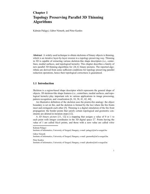
Chapter 1
Topology Preserving Parallel 3D Thinning
Algorithms
Kálmán Palágyi, Gábor Németh, and Péter Kardos
Abstract A widely used technique to obtain skeletons of binary objects is thinning,
which is an iterative layer-by-layer erosion in a topology preserving way. Thinning
in 3D is capable of extracting various skeleton-like shape descriptors (i.e., centerlines,
medial surfaces, and topological kernels). This chapter describes a family of
new parallel 3D thinning algorithms for (26,6) binary pictures. The reported algorithms
are derived from some sufficient conditions for topology preserving parallel
reduction operations, hence their topological correctness is guaranteed.
1.1 Introduction
Skeleton is a region-based shape descriptor which represents the general shape of
objects. 3D skeleton-like shape features (i.e., centerlines, medial surfaces, and topological
kernels) play important role in various applications in image processing,
pattern recognition, and visualization [6, 10, 38, 41, 42, 44].
An illustrative definition of the skeleton uses the prairie-fire analogy: the object
boundary is set on fire, and the skeleton is formed by the loci where the fire fronts
meet and extinguish each other [5]. Thinning is a digital simulation of the fire front
propagation: the border points that satisfy certain topological and geometric constraints
are deleted in iteration steps [12].
A 3D binary picture [11, 12] is a mapping that assigns a value of 0 or 1 to
each point with integer coordinates in the 3D digital space Z 3 . Points having the
value of 1 are called black points, and those with a zero value are called white
Kálmán Palágyi
Institute of Informatics, University of Szeged, Hungary, e-mail: palagyi@inf.u-szeged.hu
Gábor Németh
Institute of Informatics, University of Szeged, Hungary, e-mail: gnemeth@inf.u-szeged.hu
Péter Kardos
Institute of Informatics, University of Szeged, Hungary, e-mail: pkardos@inf.u-szeged.hu
1

2 K. Palágyi, G. Németh, P. Kardos
ones. Black points form the components of a picture, while white points form the
background and the cavities. We consider (26,6)–pictures, where 26–adjacency and
6–adjacency are, respectively, used for the components and their complement [12].
A reduction operation transforms a binary picture only by changing some black
points to white ones (which is referred to as the deletion of 1’s). A parallel reduction
operation deletes all points satisfying its condition simultaneously. A reduction
operation does not preserve topology [11] if
• any component in the input picture is split (into several components) or is completely
deleted,
• any cavity in the input picture is merged with the background or another cavity,
or
• a cavity is created where there was none in the input picture.
There is an additional concept called hole (or tunnel) in 3D pictures. A hole
(which doughnuts have) is formed of 0’s, but it is not a cavity [12]. Topology preservation
implies that eliminating or creating any hole is not allowed.
There are three types of 3D thinning algorithms for producing the three types
of skeleton-like shape features: curve–thinning algorithms are used to extract medial
lines or centerlines, surface–thinning algorithms produce medial surfaces, while
kernel–thinning algorithms are capable of extracting topological kernels. A topological
kernel is a minimal set of points that is topologically equivalent [12] to the
original object (i.e., if we remove any further point from it, then the topology is not
preserved). Note that kernel–thinning algorithms are often referred to as reductive
shrinking algorithms [9]. 3D curve-thinning and surface-thinning algorithms use
operations that delete some points which are not endpoints, since preserving endpoints
provides important geometrical information relative to the shape of the objects.
Kernel–thinning algorithms for extracting topological kernels do not take any
endpoint characterization into consideration. Medial surfaces are usually extracted
from general shapes, tubular structures can be represented by their centerlines, and
extracting topological kernels is useful in topological description.
Most of the existing thinning algorithms are parallel as the fire front propagation
is by nature parallel. These algorithms are composed of parallel reduction operations.
Parallel reduction operations delete a set of points simultaneously which may
lead to altering the topology. Note that deletion rules of parallel thinning algorithms
are generally given by matching templates. In order to verify that a given parallel
3D thinning algorithm preserves the topology for all possible (26,6) pictures, some
sufficient conditions for topology preservation have been proposed [11, 18, 36].
However, verifying these conditions usually means checking several configurations
of points, hence papers presenting thinning algorithms contain long proof parts.
Despite of complex proofs, it was claimed in [14, 45] that two parallel 3D thinning
algorithms [18, 19] are not topology preserving. That is why we propose a
safe technique for designing topologically correct parallel 3D thinning algorithms.
Our approach is based on some new sufficient conditions for topology preservation.
These conditions consider individual points (instead of point configurations) and
can be combined with various thinning strategies.

1 Topology Preserving Parallel 3D Thinning Algorithms 3
In this chapter we present 15 algorithms that are derived from the new sufficient
conditions combined with the three major strategies for parallel thinning (i.e., fully
parallel, subiteration-based, and subfield-based [8]) and three types of endpoints.
The rest of this chapter is organized as follows. Section 1.2 reviews the basic notions
and results of 3D digital topology, and we present our sufficient conditions for
topology preservation. Then, in Sect. 1.3 we propose 15 parallel 3D thinning algorithms
and their topological correctness is proved. Since fast extraction of skeletonlike
shape features is extremely important in numerous applications for large 3D
shapes, Sect. 1.4 is devoted to the efficient implementation of the proposed algorithms,
and Sect. 1.5 presents some illustrative results. In Sect. 1.6 some possible
future works and open problems are outlined. Finally, we round off the chapter with
some concluding remarks.
1.2 Topology Preserving Parallel Reduction Operations
In this section, we present new sufficient conditions for topology preservation. First
we outline some concepts of digital topology and related key results that will be
used in the sequel.
Let p be a point in the 3D digital space Z 3 . Let us denote Nj(p) (for j = 6,18,26)
the set of points that are j-adjacent to point p (see Fig. 1.1).
• ◦ •
◦✑✑ ✑✑ ✑✑ ✑✑ ✑✑
U ◦✑✑
•✑✑ ✑✑
◦✑✑ ✑✑
•✑✑
✑✑
◦ N ◦
✑✑ ✑✑ ✑✑
W p ✑✑
E
◦✑✑ ✑✑ ✑✑
S ◦✑✑
• ◦ •
◦✑✑ ✑✑ ✑✑
D ◦✑✑
•✑✑ ◦✑✑ •✑✑
✑✑
Fig. 1.1 Frequently used adjacencies in Z 3 . The set N6(p) contains point p and the six points
marked U, D, N, E, S, and W. The set N18(p) contains N6(p) and the twelve points marked by
“◦”. The set N26(p) contains N18(p) and the eight points marked by “•”
The sequence of distinct points 〈x0,x1,...,xn〉 is called a j-path (for j = 6,26) of
length n from point x0 to point xn in a non-empty set of points X if each point of
the sequence is in X and xi is j-adjacent to xi−1 for each 1 ≤ i ≤ n (see Fig. 1.1).
Note that a single point is a j-path of length 0. Two points are said to be j-connected
in the set X if there is a j-path in X between them ( j = 6,26). A set of points X is
j-connected in the set of points Y ⊇ X if any two points in X are j-connected in Y
( j = 6,26).

4 K. Palágyi, G. Németh, P. Kardos
A 3D binary (26,6) digital picture P is a quadruple P = (Z 3 ,26,6,B) [12].
Each element of Z 3 is called a point of P. Each point in B ⊆ Z 3 is called a black
point and has a value 1. Each point in Z 3 \B is called a white point and has a value 0.
An object is a maximal 26-connected set of black points, while a white component is
a maximal 6-connected set of white points. Here it is assumed that a picture contains
finitely many black points.
The lexicographical order relation “≺” between two distinct points p=(px, py, pz)
and q = (qx,qy,qz) in Z 3 is defined as follows:
p ≺ q ⇔ (pz < qz) ∨(pz = qz ∧ py < qy) ∨(pz = qz ∧ py = qy ∧ px < qx).
Let C ⊆ Z 3 be a set of points. Point p ∈ C is the smallest element of C if for any
q ∈ C\{p}, p ≺ q.
A unit lattice square is a set of four mutually 18-adjacent points in Z 3 , while a
unit lattice cube is a set of eight mutually 26-adjacent points in Z 3 .
A black point is called a border point in (26,6) pictures if it is 6-adjacent to
at least one white point. A border point p is called a U-border point if the point
marked U= u(p) in Fig. 1.1 is a white point. We can define D-, N-, E-, S-, and Wborder
points in the same way. A black point is called an interior point if it is not
a border point. A simple point in a (26,6) picture is a black point whose deletion
is a topology preserving reduction operation [12]. Note that simplicity of point p
in (26,6) pictures is a local property that can be decided by investigating the set
N26(p) [12].
Parallel reduction operations delete a set of black points and not just a single
simple point. Hence we need to consider what is meant by topology preservation
when a number of black points are deleted simultaneously.
Ma [17] gave some sufficient conditions for 3D parallel reduction operations to
preserve topology. Later, Palágyi and Kuba proposed the following simplified conditions
[36]:
Theorem 1. [36] The parallel reduction operation O is topology preserving for
(26,6) pictures if all the following conditions hold.
1. Only simple points are deleted by O.
2. Let p be any black point in a picture (Z 3 ,26,6,B) such that p is deleted by O.
Let Q ⊆ B be any set of simple points in (Z 3 ,26,6,B) such that p ∈ Q, and Q is
contained in a unit lattice square.
Then point p is simple in picture (Z 3 ,26,6,B\(Q\{p})).
3. No object contained in a unit lattice cube is deleted completely by O.
Theorem 1 provides a general method of verifying that a parallel thinning algorithm
preserves topology. In this section, we present some new sufficient conditions
for topology preservation as a basis for designing 3D parallel thinning algorithms.
Theorem 2. The parallel reduction operation O is topology preserving for (26,6)
pictures if all the following conditions hold for any black point p in any picture
(Z 3 ,26,6,B) such that p is deleted by O.

1 Topology Preserving Parallel 3D Thinning Algorithms 5
1. Point p is simple in (Z 3 ,26,6,B).
2. Let Q ⊆ B be any set of simple points in (Z 3 ,26,6,B) such that p ∈ Q, and Q is
contained in a unit lattice square.
Then point p is simple in picture (Z 3 ,26,6,B\(Q\{p})), or p is not the smallest
element of Q.
3. Point p is not the smallest element of any object C ⊆ B in (Z 3 ,26,6,B) such that
C is contained in a unit lattice cube.
Proof. It can be readily seen that if the parallel reduction operation O satisfies Condition
i of Theorem 2, then Condition i of Theorem 1 is also satisfied (i = 1,2,3).
Hence, parallel reduction operation O is topology preserving for (26,6) pictures.
⊓⊔
1.3 Variations on Parallel 3D Thinning Algorithms
In this section, 15 parallel 3D thinning algorithms are presented. These algorithms
are composed of parallel reduction operations derived from our sufficient conditions
for topology preservation (see Theorem 2).
Thinning algorithms preserve endpoints and some border points that provide relevant
geometrical information with respect to the shape of the object. Here, we
consider three types of endpoints.
Definition 1. There is no endpoint of type TK.
To standardize the notations, shrinking algorithms capable of producing topological
kernels are considered as kernel-thinning algorithms, where no endpoint is
preserved, hence we use endpoints of type TK (i.e., the empty set of the endpoints).
Definition 2. A black point p in picture (Z 3 ,26,6,B) is a curve-endpoint of type
CE if (N26(p)\{p}) ∩ B contains exactly one point (i.e., p is 26-adjacent to exactly
one further black point).
Endpoints of type CE have been considered by numerous existing 3D curvethinning
algorithms [26, 27, 28, 34, 35, 36, 38].
Definition 3. A black point p in picture (Z 3 ,26,6,B) is a surface-endpoint of type
SE if there is no interior point in N26(p) ∩ B.
Note that the characterization of endpoints SE is applied in some existing
surface-thinning algorithms [24, 26, 27, 28, 31, 33, 37].
In the rest of this section we present parallel 3D thinning algorithms composed
of parallel reduction operations that satisfy Theorem 2.

6 K. Palágyi, G. Németh, P. Kardos
1.3.1 Fully Parallel Algorithms
In fully parallel algorithms, the same parallel reduction operation is applied in each
iteration step [1, 15, 16, 18, 19, 33, 45].
The scheme of the proposed fully parallel thinning algorithm 3D-FP-ε using endpoint
of type ε is sketched in Algorithm 1 (ε ∈ { TK, CE, SE }). Note that Palágyi
and Németh reported three fully parallel 3D surface-thinning algorithms in [37], but
they were based on different sufficient conditions.
Algorithm 1 Algorithm 3D-FP-ε
1: Input: picture (Z 3 ,26,6,X)
2: Output: picture (Z 3 ,26,6,Y)
3: Y = X
4: repeat
5: // one iteration step
6: D = {p | p is 3D-FP-ε-deletable in Y }
7: Y = Y \ D
8: until D = /0
3D-FP-ε-deletable points are defined as follows:
Definition 4. A black point is 3D-FP-ε-deletable if it is not an endpoint of type ε,
and all conditions of Theorem 2 hold (ε ∈ { TK, CE, SE }).
We have the following theorem.
Theorem 3. Algorithm 3D-FP-ε (ε ∈ { TK, CE, SE }) is topology preserving for
(26,6) pictures.
Proof. Deletable points of the proposed fully parallel algorithms (see Definition 4)
are derived directly from conditions of Theorem 2. Hence, all of the three algorithms
are topology preserving. ⊓⊔
Note that all objects contained in a unit lattice cube are formed of endpoints of
type SE. Hence, Condition 3 of Theorem 2 can be ignored in algorithm 3D-FP-SE.
1.3.2 Subiteration-based Algorithms
In subiteration-based (or frequently referred to as directional) thinning algorithms,
an iteration step is decomposed into k successive parallel reduction operations according
to k deletion directions [8]. If the current deletion direction is d, then a set
of d-border points can be deleted by the parallel reduction operation assigned to it.
Since there are six kinds of major directions in 3D cases, 6–subiteration algorithms
were generally proposed [2, 7, 13, 20, 25, 34, 43, 46]. Moreover, 3–subiteration

1 Topology Preserving Parallel 3D Thinning Algorithms 7
[30, 31, 32], 8–subiteration [35], and 12–subiteration [36] algorithms have also been
developed for this task.
In what follows, we present three examples of parallel 3D 6–subiteration thinning
algorithms. Algorithm 2 sketches the scheme of 3D 6-subiteration parallel thinning
algorithm 3D-6-SI-ε that uses the endpoint of type ε (ε ∈ { TK, CE, SE }).
Algorithm 2 Algorithm 3D-6-SI-ε
1: Input: picture (Z 3 ,26,6,X)
2: Output: picture (Z 3 ,26,6,Y)
3: Y = X
4: repeat
5: // one iteration step
6: for each i ∈ {U,D,N,E,S,W} do
7: // subiteration for deleting some i-border points
8: D(i) = { p | p is a 3D-6-SI-i-ε-deletable point in Y }
9: Y = Y \ D(i)
10: end for
11: until D(U) ∪ D(D) ∪ D(N) ∪ D(E) ∪ D(S) ∪ D(W) = /0
The ordered list of deletion directions 〈U,D,N,E,S,W〉 [7, 34] is considered in
the proposed algorithm 3D-6-SI-ε (ε ∈ { TK, CE, SE }). Note that subiterationbased
thinning algorithms are not invariant under the order of deletion directions
(i.e., choosing different orders may yield various results).
In the first subiteration of our 6-subiteration thinning algorithms, the set of 3D-
6-SI-U-ε-deletable points are deleted simultaneously, and the set of 3D-6-SI-W-εdeletable
points are deleted in the last (i.e., the 6th) subiteration. Now we lay down
3D-6-SI-U-ε-deletable points.
Definition 5. A black point p in picture (Z 3 ,26,6,X) is 3D-6-SI-U-ε-deletable if
all of the following conditions hold:
1. Point p is a simple and U-border point, but it is not an endpoint of type ε in
picture (Z 3 ,26,6,X).
2. Let A (p) be the family of the following 13 sets (see Fig. 1.2b):
{e}, {s}, {se}, {sw}, {dn}, {de}, {ds}, {dw},
{e,s}, {e,se}, {s,se}, {s,sw},
{e,s,se}.
For any set A in the family A (p) composed of simple and U-border points, but
not endpoints of type ε in picture (Z 3 ,26,6,X), point p remains simple in picture
(Z 3 ,26,6,X\A).
3. Let B(p) be the family of the following 42 objects in picture (Z 3 ,26,6,X) (see
Fig. 1.2c):
{a,h}, {b,g}, {c, f }, {d,e},
{a,h,b}, {a,h,c}, {a,h, f }, {a,h,g}, {b,g,a}, {b,g,d}, {b,g,e}, {b,g,h},
{c, f,a}, {c, f,d}, {c, f,e}, {c, f,h}, {d,e,b}, {d,e,c}, {d,e, f }, {d,e,g},
{b,c,h}, {d,g, f }, {a,d, f }, {b,e,h}, {b,c,e}, {a, f,g}, {a,d,g}, {c,e,h},

8 K. Palágyi, G. Németh, P. Kardos
{a,h,b,c}, {a,h,b,g}, {a,h,c, f }, {a,h, f,g}, {b,g,a,d}, {b,g,d,e}, {b,c,e,h},
{b,g,e,h}, {c, f,a,d}, {c, f,d,e}, {c, f,e,h}, {d,e,b,c}, {d,e, f,g}, {a,d, f,g}.
Point p is not the smallest element of any object in B(p).
y
z
x
✑ ✑ ✑ ✑ ✑ ✑ ✑ ✑ ✑ ✑ ✑ ✑ ✑ ✑ ✑ ✑ ✑ ✑ un
uw u ue
us
nw n ne
w p e
sw s se
dn
dw d de
✑
ds
✑
✑ ✑ ✑ ✑ ✑ ✑ ✑ ✑ ✑ a b c
✑ ✑ a b
✑
c d
✑ ✑ ✑ ✑ e f
g ✑
h
✑
Fig. 1.2 The considered right-handed 3D coordinate system (a). Notation for the points in N18(p)
(b). Notation for the points in a unit lattice cube (c)
Note that the deletable points at the remaining five subiterations can be derived
from 3D-6-SI-U-ε-deletable points (assigned to the deletion direction U, see Definition
5) by reflexions and rotations.
Theorem 4. Algorithm 3D-6-SI-ε (ε ∈ { TK, CE, SE }) is topology preserving for
(26,6) pictures.
Proof. Without loss of generality, it is sufficient to prove that the first subiteration of
algorithm 3D-6-SI-ε is topology preserving. To this end, we show that the parallel
reduction operation T that deletes 3D-6-SI-U-ε-deletable points (ε ∈ { TK, CE,
SE }) satisfies all conditions of Theorem 2.
1. Operation T may delete simple points by Condition 1 of Definition 5. Hence
Condition 1 of Theorem 2 is satisfied.
2. It is easy to see that the family A (p) (see Condition 2 of Definition 5 and Fig.
1.2a-b) contains all possible sets of simple U-border points that are considered
by Condition 2 of Theorem 2. Therefore, this latter condition is satisfied.
3. It can be readily seen that the family of objects B(p) (see Condition 3 of Definition
5 and Fig. 1.2c) contains all possible objects of U-border points that are
considered in Condition 3 of Theorem 2. Hence, this last condition is satisfied.
Since objects contained in a unit lattice cube are composed of endpoints of type
SE, Condition 3 of Definition 5 can be ignored in algorithm 3D-6-SI-SE. ⊓⊔

1 Topology Preserving Parallel 3D Thinning Algorithms 9
1.3.3 Subfield-based Algorithms
The third type of parallel thinning algorithms applies subfield-based technique [8].
In existing subfield-based parallel 3D thinning algorithms, the digital space Z 3 is
partitioned into two [21, 22, 26], four [23, 27], and eight [3, 27] subfields which are
alternatively activated. At a given iteration step of a k-subfield algorithm, k successive
parallel reduction operations associated to the k subfields are performed. In each
of them, some border points in the active subfield can be designated for deletion.
Let us denote SFk(i) the i-th subfield if Z 3 is partitioned into k subfields (k =
2,4,8; i = 0,...,k − 1). SFk(i) is defined formally as follows:
SF2(i) = { (px, py, pz)| (px + py + pz mod 2) = i },
SF4(i) = { (px, py, pz)| (px+1 mod 2) ·[2 ·(py mod 2)+(pz mod 2)]+
(px mod2) ·[2 ·(py+1 mod 2)+(pz+1 mod 2)] = i },
SF8(i) = { (px, py, pz)| 4 ·(px mod 2)+2·(py mod 2)+(pz mod 2) = i }
The considered divisions are illustrated in Fig. 1.3.
1 0 1
✑
✑
✑
0 1 0
✑
✑
✑
1 0 1
0 1 0
✑ ✑ ✑
1 0 1
✑ ✑ ✑
0 1 0
1 0 1
✑ ✑ ✑
0 1 0
✑ ✑ ✑
1 0 1
0 3 0
✑ ✑ ✑
2 1 2
✑ ✑ ✑
0 3 0
1 2 1
✑ ✑ ✑
3 0 3
✑ ✑ ✑
1 2 1
0 3 0
✑ ✑ ✑
2 1 2
✑ ✑ ✑
0 3 0
7 3 7
✑
✑
✑
5 1 5
✑
✑
✑
7 3 7
6 2 6
✑ ✑ ✑
4 0 4
✑ ✑ ✑
6 2 6
7 3 7
✑ ✑ ✑
5 1 5
✑ ✑ ✑
7 3 7
a b c
Fig. 1.3 The divisions of Z 3 into 2 (a), 4 (b), and 8 (c) subfields. If partitioning into k subfields is
considered, then points marked “i” are in the subfield SFk(i) (k = 2,4,8; i = 0,1,...,k − 1)
Proposition 1. For the 2-subfield case (see Fig. 1.3a), two points p and q ∈ N26(p)
are in the same subfield, if q ∈ N18(p)\N6(p).
Proposition 2. For the 4-subfield case (see Fig. 1.3b), two points p and q ∈ N26(p)
are in the same subfield, if q ∈ N26(p)\N18(p).
Proposition 3. For the 8-subfield case (see Fig. 1.3c), two points p and q ∈ N26(p)
are not in the same subfield.
In order to reduce the noise sensitivity and the number of skeletal points (without
overshrinking the objects), Németh, Kardos, and Palágyi introduced a new subfieldbased
thinning scheme [26]. It takes the endpoints into consideration at the begin-

10 K. Palágyi, G. Németh, P. Kardos
ning of iteration steps, instead of preserving them in each parallel reduction operation
as it is accustomed in the conventional subfield-based thinning scheme.
Next, we present nine parallel 3D subfield-based thinning algorithms. The scheme
of the subfield-based parallel thinning algorithm 3D-k-SF-ε with iteration-level endpoint
checking using endpoint of type ε is sketched in Algorithm 3 (with k = 2,4,8;
ε ∈ { TK, CE, SE }).
Algorithm 3 Algorithm 3D-k-SF-ε
1: Input: picture (Z 3 ,26,6,X)
2: Output: picture (Z 3 ,26,6,Y)
3: Y = X
4: repeat
5: // one iteration step
6: E = { p | p is a border point, but not an endpoint of type ε in Y }
7: for i = 0 to k − 1 do
8: // subfield SFk(i) is activated
9: D(i) = { q | q is a 3D-SF-k-deletable point in E ∩ SFk(i) }
10: Y = Y \ D(i)
11: end for
12: until D(0) ∪ D(1) ∪... ∪ D(k − 1) = /0
The 3D-SF-k-deletable points are defined as follows (k = 2,4,8):
Definition 6. A black point p is 3D-SF-k-deletable (k = 2,4,8) in picture (Z 3 ,26,6,X)
if all of the following conditions hold:
1. Point p is simple in (Z 3 ,26,6,X).
2. If k = 2, then point p is simple in picture (Z 3 ,26,6,X\{q}) for any simple point
q such that q ∈ N18(p)\N6(p) and p ≺ q.
3. • If k = 2, then point p is not the smallest element of the ten objects depicted in
Fig. 1.4.
• If k = 4, then point p is not the smallest element of the four objects depicted
in Fig. 1.5.
Theorem 5. Algorithm 3D-k-SF-ε (k = 2,4,8; ε ∈ { TK, CE, SE }) is topology
preserving for (26,6) pictures.
Proof. To prove it, we show that the parallel reduction operation T that deletes
3D-SF-k-deletable points satisfies all conditions of Theorem 2.
1. Operation T may delete simple points by Condition 1 of Definition 6. Hence
Condition 1 of Theorem 2 is satisfied.
2. • Let k = 2 and let p ∈ SF2(i) be any black point in picture (Z 3 ,26,6,X) that is
deleted by T (i = 0,1).
Let Q ⊆ X ∩SF2(i) be any set of black points in (Z 3 ,26,6,X) such that p ∈ Q,
Q is contained in a unit lattice square, and each point in Q\{p} is simple in
picture (Z 3 ,26,6,X).

1 Topology Preserving Parallel 3D Thinning Algorithms 11
• ◦
◦✑ ✑ •✑
✑
◦ •
◦✑ ◦ ✑
◦ •
•✑ ✑ ◦✑
✑
• ◦
◦✑ ◦ ✑
• ◦
◦ ✑ • ✑
◦ ◦
•✑ ◦ ✑
◦ •
• ✑ ◦ ✑
◦ ◦
◦✑ • ✑
• ◦
◦✑ ✑ ◦✑
✑
◦ •
•✑ ◦ ✑
◦ •
◦✑ ✑ ◦✑
✑
• ◦
◦✑ • ✑
• ◦
◦✑ ✑ •✑
✑
◦ •
•✑ ◦ ✑
◦ •
•✑ ✑ ◦✑
✑
• ◦
◦✑ • ✑
◦ ◦
◦✑ ✑ •✑
✑
◦ •
•✑ ◦ ✑
◦ ◦
•✑ ✑ ◦✑
✑
• ◦
◦✑ • ✑
Fig. 1.4 The ten objects that are taken into consideration by 2-subfield algorithms. Notations: each
point marked by “•” is a black point; each point marked by “◦” is a white point. (Note that each
of these objects is contained in a unit lattice cube.)
• ◦
◦ ✑ ◦ ✑
◦ ◦
◦✑ • ✑
◦ •
◦✑ ✑ ◦✑
✑
◦ ◦
•✑ ◦ ✑
◦ ◦
◦ ✑ • ✑
• ◦
◦✑ ◦ ✑
◦ ◦
•✑ ✑ ◦✑
✑
◦ •
◦✑ ◦ ✑
Fig. 1.5 The four objects considered by 4-subfield algorithms. Notations: each point marked “•”
is a black point; each point marked “◦” is a white point. (Note that each of these objects is contained
in a unit lattice cube.)
Then Q = /0 or Q = {q} by Proposition 1, and such kind of sets are considered
by Condition 2 of Definition 6. Hence Condition 2 of Theorem 2 is satisfied.
• Let k = 4 and let p ∈ SF4(i) be any black point in picture (Z 3 ,26,6,X) that is
deleted by T (i = 0,1,2,3).
Let Q ⊆ X ∩SF4(i) be any set of black points in (Z 3 ,26,6,X) such that p ∈ Q,
Q is contained in a unit lattice square, and each point in Q\{p} is simple in
picture (Z 3 ,26,6,X).
Then Q = /0 by Proposition 2. Hence Condition 2 of Theorem 2 is satisfied.
• Let k = 8 and let p ∈ SF8(i) be any black point in picture (Z 3 ,26,6,X) that is
deleted by T (i = 0,1,...,7).
Let Q ⊆ X ∩SF8(i) be any set of black points in (Z 3 ,26,6,X) such that p ∈ Q,
Q is contained in a unit lattice square, and each point in Q\{p} is simple in
picture (Z 3 ,26,6,X).
Then Q = /0 by Proposition 3. Hence Condition 2 of Theorem 2 is satisfied.
3. • Let k = 2 and let C ⊆ X ∩ SF2(i) be any object in picture (Z 3 ,26,6,X) that is
contained in a unit lattice cube (i = 0,1).
It can be readily seen by Proposition 1 that all the ten possible cases for such
objects are depicted in Fig. 1.4, and these objects cannot be deleted completely
by Condition 3 of Definition 6.
Hence Condition 3 of Theorem 2 is satisfied.
• Let k = 4 and let C ⊆ X ∩ SF4(i) be any object in picture (Z 3 ,26,6,X) that is
contained in a unit lattice cube (i = 0,1,2,3).

12 K. Palágyi, G. Németh, P. Kardos
It can be readily seen by Proposition 2 that all the four possible cases for such
objects are depicted in Fig. 1.5, and these objects cannot be deleted completely
by Condition 3 of Definition 6.
Hence Condition 3 of Theorem 2 is satisfied.
• Let k = 8 and let C ⊆ X ∩ SF8(i) be any object in picture (Z 3 ,26,6,X) that is
contained in a unit lattice cube (i = 0,1,...,7).
It is easy to see that there is no such an object by Proposition 3.
Hence Condition 3 of Theorem 2 is satisfied. ⊓⊔
Since objects contained in a unit lattice cube are composed of endpoints of
type SE, Condition 3 of Definition 6 can be ignored in algorithm 3D-k-SF-SE
(k = 2,4,8).
1.4 Implementation
One may think that the proposed algorithms are time consuming and it is rather
difficult to implement them. That is why we outline a method for implementing any
3D fully parallel thinning algorithm on a conventional sequential computer. This
framework is fairly general, as similar schemes can be used for the other classes of
parallel algorithms and some sequential 3D thinning algorithms [38, 33, 37].
The proposed method uses a pre–calculated look-up-table to encode simple
points. In addition, two lists are used to speed up the process: one for storing the
border points in the current picture (since thinning can only delete border points,
thus the repeated scans/traverses of the entire array storing the picture are avoided);
the other list is to collect all deletable points in the current phase of the process.
At each iteration, the deletable points are found and deleted, and the list of border
points is updated accordingly. The algorithm terminates when no further update is
required.
For simplicity, the pseudocode of the proposed 3D fully parallel thinning algorithms
is given (see Algorithm 4). The subiteration-based and the subfield-based
variants can be implemented in similar ways.
The two input parameters of the procedure are array A which stores the input
picture to be thinned and the type of the considered endpoints ε. In input array A,
the value “1” corresponds to black points and the value “0” denotes white ones.
According to the proposed scheme, the input and the output pictures can be stored
in the same array, hence array A will contain the resultant structure.
First, the input picture is scanned and all the border points are inserted into the
list border list. We should mention here that it is the only time consuming scanning.
Since only a small part of points in a usual picture belong to the objects, the thinning
procedure is much faster if we just deal with the set of border points in the
actual picture. This subset of object points is stored in border list (i.e., a dynamic
data structure). The border list is then updated: if a border point is deleted, then
all interior points that are 6-adjacent to it become border points. These brand new

1 Topology Preserving Parallel 3D Thinning Algorithms 13
Algorithm 4 Fully parallel thinning algorithm
1: Input: array A and endpoint characterization ε
2: Output: array A
3: // collect border points
4: border list =< empty list >
5: for each p = (x,y,z) in A do
6: if p is border point then
7: border list = border list + < p >
8: A[x,y,z] = 2
9: end if
10: end for
11: // thinning
12: repeat
13: deleted = 0
14: deletable list = < empty list >
15: // checking Condition 1 of Theorem 2
16: for each point p = (x,y,z) in border list do
17: if p is a simple point and not an endpoint of type ε then
18: deletable list = deletable list + < p >
19: A[x,y,z] = 3
20: else
21: A[x,y,z] = 2
22: end if
23: end for
24: // checking Condition 2 of Theorem 2
25: for each point p in deletable list do
26: if deletion p does not satisfy Condition 2 of Theorem 2 then
27: deletable list = deletable list − < p >
28: end if
29: end for
30: // checking Condition 3 of Theorem 2
31: for each point p in deletable list do
32: if deletion p does not satisfy Condition 3 of Theorem 2 then
33: deletable list = deletable list − < p >
34: end if
35: end for
36: // deletion
37: for each point p = (x,y,z) in deletable list do
38: A[x,y,z] = 0
39: border list = border list − < p >
40: deleted = deleted+1
41: // update border list
42: for each point q = (x ′ ,y ′ ,z ′ ) that is 6-adjacent to p do
43: if A[x ′ ,y ′ ,z ′ ] = 1 then
44: A[x ′ ,y ′ ,z ′ ] = 2
45: border list = border list + < q >
46: end if
47: end for
48: end for
49: until deleted = 0

14 K. Palágyi, G. Németh, P. Kardos
border points of the actual picture are added to the border list. In order to avoid
storing more than one copy of a border point in border list, array A represents a
four-colour picture during the thinning process: the value “0” corresponds to the
white points, the value “1” corresponds to (black) interior points, the value “2” is
assigned to all (black) border points in the actual picture (added to border list), and
the value “3” corresponds to points that are added to the deletable list (i.e., a sublist
of border list).
The kernel of the repeat cycle corresponds to one iteration step of the thinning
process. The number of deleted points is stored in the variable called deleted. The
thinning process terminates when no more points can be deleted (i.e., no further
changes occur). After thinning, all points having a nonzero value belong to the produced
skeleton-like shape feature.
Simple points in (26,6) pictures can be locally characterized; the simplicity of
a point p can be decided by examining the set N26(p) [12]. There are 2 26 possible
configurations in the 3 × 3 × 3 neighborhood if the central point is not considered.
Hence we can assign an index (i.e., a non-negative integer code) for each possible
configuration and address a pre-calculated (unit time access) look-up-table having
2 26 entries of 1 bit in size, therefore, it requires only 8 megabytes storage space in
memory.
By adapting this efficient implementation method, our algorithms can be well
applied in practice: they are capable of extracting skeleton-like shape features from
large 3D pictures containing 1,000,000 object points within one second on a standard
PC.
1.5 Results
The proposed 15 algorithms were tested on objects of different shapes. Here we
present some of them (see Figs. 1.6-1.12). The pairs of numbers in parentheses are
the counts of object points in the produced skeleton-like structure and the parallel
speed (i.e., the number of the performed parallel reduction operations [8]).
1.6 Possible Future Works and Open Problems
In this section, we will outline some possible future works and open problems concerning
parallel 3D thinning.
• Conventional thinning algorithms preserve endpoints to provide important geometric
information relative to the object to be represented. Bertrand and Couprie
proposed an alternative strategy [4]. They developed a sequential thinning
scheme based on a generalization of curve/surface interior points that are called
isthmuses. Isthmuses are dynamically detected and accumulated in a constraint
set of non-simple points.

1 Topology Preserving Parallel 3D Thinning Algorithms 15
original image 3D-FP-TK (194, 114)
3D-6-SI-TK (200, 150) 3D-2-SF-TK (181, 200)
3D-4-SF-TK (171, 324) 3D-8-SF-TK (185, 496)
Fig. 1.6 A 191 × 96 × 114 image of a hand and its topological kernels produced by the five proposed
parallel 3D kernel–thinning algorithms. The original image contains 455295 black points.
Since the original object contains a hole, there are holes in its topological kernels, too

16 K. Palágyi, G. Németh, P. Kardos
original image 3D-FP-CE (870, 41)
3D-6-SI-CE (943, 96) 3D-2-SF-CE (875, 38)
3D-4-SF-CE (804, 108) 3D-8-SF-CE (838, 216)
Fig. 1.7 A 135 × 86 × 191 image of a dragon and its centerlines produced by the five proposed
parallel 3D curve-thinning algorithms. The original image contains 423059 black points

1 Topology Preserving Parallel 3D Thinning Algorithms 17
original image 3D-FP-CE (1481, 45)
3D-6-SI-CE (1465, 186) 3D-2-SF-CE (1647, 116)
3D-4-SF-CE (1557, 208) 3D-8-SF-CE (1559, 408)
Fig. 1.8 A 380×287×271 image of a deer head and its centerlines produced by the five proposed
parallel 3D curve-thinning algorithms. The original image contains 1658641 black points

18 K. Palágyi, G. Németh, P. Kardos
original image 3D-FP-CE (1218, 48)
3D-6-SI-CE (1323, 114) 3D-2-SF-CE (1248, 54)
3D-4-SF-CE (1241, 108) 3D-8-SF-CE (1230, 208)
Fig. 1.9 A 103×381×255 image of a helicopter and its centerlines produced by the five proposed
parallel 3D curve-thinning algorithms. The original image contains 273743 black points
The very first parallel 3D isthmus-based curve-thinning algorithm was designed
by Raynal and Couprie [39]. Each iteration step of their 6-subiteration algorithm
consists of two phases:
1. Updating the constraint set, by adding points detected as isthmuses;
2. Removing “deletable” points which are not in the constraint set.
Raynal and Couprie gave these “deletable” points by 3 × 3 × 3 matching templates,
and proved that simultaneous deletion of “deletable” points is a topology
preserving reduction operation. Hence their algorithm is topology preserving.
In a forthcoming work, we are going to combine our sufficient conditions for
topology preservation (see Theorem 2) with various parallel thinning strategies
(i.e., fully parallel, subiteration-based, and subfield-based) and some characterizations
of isthmuses to generate new parallel 3D curve-thinning and surfacethinning
algorithms.
• The 3D parallel thinning algorithms presented in this chapter are based on Theorem
2 (i.e., some sufficient conditions for topology preservation). Conditions 2
and 3 of Theorem 2 are “asymmetric”, since points that are the smallest elements
of some sets may not be deleted. It is easy to see that the following theorem
provides “symmetric” conditions for topology preservation.

1 Topology Preserving Parallel 3D Thinning Algorithms 19
original image 3D-FP-SE (25022, 18)
3D-6-SI-SE (24873, 78) 3D-2-SF-SE (17825, 34)
3D-4-SF-SE (17235, 72) 3D-8-SF-SE (17527, 136)
Fig. 1.10 A 45 × 191 × 191 image of a gear and its medial surfaces produced by the five proposed
parallel 3D surface–thinning algorithms. The original image contains 596360 black points

20 K. Palágyi, G. Németh, P. Kardos
original image 3D-FP-SE (24663, 44)
3D-6-SI-SE (10496, 168) 3D-2-SF-SE (13655, 88)
3D-4-SF-SE (12490, 176) 3D-8-SF-SE (12556, 352)
Fig. 1.11 A 285×285×88 image of a camel and its medial surfaces produced by the five proposed
parallel 3D surface–thinning algorithms. The original image contains 1088458 black points

1 Topology Preserving Parallel 3D Thinning Algorithms 21
original image 3D-FP-SE (76359, 41)
3D-6-SI-SE (60000, 192) 3D-2-SF-SE (48335, 82)
3D-4-SF-SE (44508, 160) 3D-8-SF-SE (47088, 320)
Fig. 1.12 A 122 × 93 × 284 image of a car and its medial surfaces produced by the five proposed
parallel 3D surface–thinning algorithms. The original image contains 1321764 black points

22 K. Palágyi, G. Németh, P. Kardos
Theorem 6. The parallel reduction operation O is topology preserving for (26,6)
pictures if all the following conditions hold for any black point p in any picture
(Z 3 ,26,6,B) such that p is deleted by O.
1. Point p is simple in (Z 3 ,26,6,B).
2. Let Q ⊆ B be any set of simple points in (Z 3 ,26,6,B) such that p ∈ Q, and Q
is contained in a unit lattice square.
Then point p is simple in picture (Z 3 ,26,6,B\(Q\{p})).
3. Point p is not an element of any object C ⊆ B in (Z 3 ,26,6,B) such that C is
contained in a unit lattice cube.
In a future work, we plan to combine alternative sufficient conditions for topology
preservation with parallel thinning strategies to generate further classes of
3D parallel thinning algorithms.
• Unfortunately, skeletonization methods (including thinning) are rather sensitive
to coarse object boundaries, hence the produced skeletons generally contain some
false segments. In order to overcome this problem, unwanted skeletal parts are
usually removed by a pruning process as a post-processing step [40]. In [29], we
presented a new thinning scheme for reducing the noise sensitivity of 3D thinning
algorithms. It uses iteration-by-iteration smoothing which removes some border
points being considered as extremities.
We are going to design new topology preserving parallel contour smoothing operations,
and combine our 3D parallel thinning algorithms (based on sufficient
conditions for topology preservation) with iteration-by-iteration smoothing.
• It is easy to see that subiteration-based and subfield-based parallel thinning
schemes are not invariant under the order of deletion directions and subfield activations,
respectively. It means that choosing different orders of directions may
yield various results in subiteration-based algorithms, and varieties of skeletonlike
shape features can be produced by a subfield-based algorithm with diverse
orders of the active subfields.
Neither order-independent subiteration-based nor subfield-based parallel thinning
algorithms have been proposed. We are going to deal with this unsolved
problem (i.e., we plan to construct subiteration-based and subfield-based algorithms
that produce the same result for any order of deletion directions and subfield
activation).
1.7 Concluding Remarks
Fast and reliable extraction of skeleton-like shape features (i.e., medial surface, centerline,
and topological kernel) is extremely important in numerous applications for
large 3D shapes. In this chapter we presented a variety of parallel 3D thinning algorithms
and their efficient implementation. They are based on some sufficient conditions
for topology preserving parallel reduction operations, hence their topological

1 Topology Preserving Parallel 3D Thinning Algorithms 23
correctness is guaranteed. The algorithms are based on different characterizations
of endpoints. Additional types of endpoints coupled with sufficient conditions for
topology preservation yield newer thinning algorithms.
Acknowledgement
This research was supported by the TÁMOP-4.2.2/08/1/2008-0008 program of
the Hungarian National Development Agency, the European Union and the European
Regional Development Fund under the grant agreement TÁMOP-4.2.1/B-
09/1/KONV-2010-0005, and the grant CNK80370 of the National Office for Research
and Technology (NKTH) & the Hungarian Scientific Research Fund (OTKA).
References
1. Arcelli, C., Sanniti di Baja, G., Serino, L.: New removal operators for surface skeletonization.
In: Proc. 13th Int. Conf. Discrete Geometry for Computer Imagery, DGCI 2006, Lecture Notes
in Computer Science, Vol. 4245, pp. 555-566. Springer, Heidelberg (2006)
2. Bertrand, G.: A parallel thinning algorithm for medial surfaces. Pattern Recognition Letters
16, 979–986 (1995)
3. Bertrand, G., Aktouf, Z.: A 3D thinning algorithm using subfields. In: SPIE Proc. of Conf. on
Vision Geometry, pp. 113-124. (1994)
4. Bertrand, G., Couprie, M.: Transformations topologiques discrètes. In: D. Coeurjolly, A. Montanvert,
J. Chassery (eds.), Géométrie discrète et images numériques, pp. 187-209. Hermès
(2007)
5. Blum, H.: A transformation for extracting new descriptors of shape. In: W. Wathen-Dunn (ed.),
Models for the Perception of Speech and Visual Form, pp. 362-380. MIT Press, Cambridge
(1967)
6. Gomberg, B.R., Saha, P.K., Song, H.K., Hwang, S.N., Wehrli, F.W.: Topological analysis of
trabecular bone MR images. IEEE Transactions on Medical Imaging 19, 166–174 (2000)
7. Gong, W.X., Bertrand G.: A simple parallel 3D thinning algorithm. In: Proc. 10th IEEE Internat.
Conf. on Pattern Recognition, ICPR’90, pp. 188-190. (1990)
8. Hall, R. W.: Parallel Connectivity-Preserving Thinning Algorithms. In: Kong, T. Y. and Rosenfeld,
A. (eds.), Topological Algorithms for Digital Image Processing, pp. 145-179. Elsevier
Science B. V., Amsterdam (1996)
9. Hall, R. W., Kong, T. Y., Rosenfeld, A.: Shrinking Binary Images. In: Kong, T. Y. and Rosenfeld,
A. (eds.), Topological Algorithms for Digital Image Processing, pp. 31-98. Elsevier Science
B. V., Amsterdam (1996)
10. Itoh, T., Yamaguchi, Y., Koyamada, K.: Fast isosurface generation using the volume thinning
algorithm. IEEE Transactions on Visualization and Computer Graphics 7, 32–46 (2001)
11. Kong, T.Y.: On topology preservation in 2–d and 3–d thinning. International Journal of Pattern
Recognition and Artificial Intelligence 9, 813–844 (1995)
12. Kong, T.Y., Rosenfeld, A.: Digital topology: Introduction and survey. Computer Vision,
Graphics, and Image Processing 48, 357–393 (1989)
13. Lee, T., Kashyap, R.L., Chu, C.: Building skeleton models via 3–D medial surface/axis thinning
algorithms. CVGIP: Graphical Models and Image Processing 56, 462–478 (1994)
14. Lohou, C.: Detection of the non-topology preservation of Ma’s 3D surface-thinning algorithm,
by the use of P-simple points. Pattern Recognition Letters 29, 822–827 (2008)

24 K. Palágyi, G. Németh, P. Kardos
15. Lohou C., Dehos, J.: An automatic correction of Mas thinning algorithm based on P-simple
points. Journal of Mathematical Imaging and Vision 36, 54–62 (2010)
16. Lohou C., Dehos, J.: Automatic correction of Ma and Sonkas thinning algorithm using Psimple
points. IEEE Transactions on Pattern Analysis and Machine Intelligence 32, 1148–
1152 (2010)
17. Ma, C.M.: On topology preservation in 3D thinning. CVGIP: Image Understanding 59, 328–
339 (1994)
18. Ma, C.M.: A 3D fully parallel thinning algorithm for generating medial faces. Pattern Recognition
Letters 16, 83–87 (1995)
19. Ma, C.M., Sonka, M.: A fully parallel 3D thinning algorithm and its applications. Computer
Vision and Image Understanding 64, 420–433 (1996)
20. Ma, C.M., Wan, S-Y.: Parallel thinning algorithms on 3D (18,6) binary images. Computer
Vision Image Understanding 80, 364–378 (2000)
21. Ma, C.M., Wan, S.Y.: A medial-surface oriented 3-d two-subfield thinning algorithm. Pattern
Recognition Letters 22, 1439–1446 (2001)
22. Ma, C.M., Wan, S.Y., Chang, H.K.: Extracting medial curves on 3D images. Pattern Recognition
Letters 23, 895–904 (2002)
23. Ma, C.M., Wan, S.Y., Lee, J.D.: Three-dimensional topology preserving reduction on the 4subfields.
IEEE Transaction on Pattern Analysis and Machine Intelligence 24, 1594–1605
(2002)
24. Manzanera, A., Bernard, T.M., Pretêux, F., Longuet, B.: Medial faces from a concise 3D thinning
algorithm. In: Proc. 7th IEEE Int. Conf. Computer Vision, ICCV’99, pp. 337-343. (1999)
25. Mukherjee, J., Das, P.P., Chatterjee, B.N.: On connectivity issues of ESPTA. Pattern Recognition
Letters 11, 643–648 (1990)
26. Németh, G., Kardos, P., Palágyi, K.: Topology preserving 2-subfield 3D thinning algorithms.
In: Proc. 7th IASTED Int. Conf. Signal Processing, Pattern Recognition and Applications, pp.
310-316. (2010)
27. Németh, G., Kardos, P., Palágyi, K.: Topology preserving 3D thinning algorithms using four
and eight subfields. In: Proc. International Conference on Image Analysis and Recognition,
ICIAR 2010. LNCS, vol. 6111, pp. 316-325. Springer, Heidelberg (2010)
28. Németh, G., Kardos, P., Palágyi, K.: A family of topology-preserving 3D parallel 6subiteration
thinning algorithms. In: Proc. 14th International Workshop on Combinatorial
Image Analysis IWCIA’2011, Madrid, Spain, Lecture Notes in Computer Science 6636, pp.
17-30. Springer, Heidelberg (2011)
29. Németh, G., Kardos, P., Palágyi, K.: Thinning combined with iteration-by-iteration smoothing
for 3D binary images. Graphical Models, in press
30. Palágyi, K.: A 3-subiteration 3D thinning algorithm for extracting medial surfaces. Pattern
Recognition Letters 23, 663–675 (2002)
31. Palágyi, K.: A 3-Subiteration Surface-Thinning Algorithm. In: Proc. 12th Int. Conf. Computer
Analysis of Images and Patterns, CAIP 2007, Vienna, Austria, Lecture Notes in Computer
Science 4673, pp. 628-635. Springer, Heidelberg (2007)
32. Palágyi, K.: A subiteration-based surface-thinning algorithm with a period of three. In: F.
Hamprecht, B. Jähne, Ch. Schnörr (eds.), Lecture Notes in Computer Science 4713, pp. 294–
303. Springer, Heidelberg (2007)
33. Palágyi, K.: A 3D fully parallel surface-thinning algorithm. Theoretical Computer Science
406, 119–135 (2008)
34. Palágyi, K., Kuba, A.: A 3D 6–subiteration thinning algorithm for extracting medial lines.
Pattern Recognition Letters 19, 613–627 (1998)
35. Palágyi, K., Kuba, A.: Directional 3D thinning using 8 subiterations. In: Proc. 8th Int. Conf. on
Discrete Geometry for Computer Imagery, DGCI’99, Marne-la-Valle, France, Lecture Notes
in Computer Science 1568, pp. 325-336. Springer, Heidelberg (1999)
36. Palágyi, K., Kuba, A.: A parallel 3D 12–subiteration thinning algorithm. Graphical Models
and Image Processing 61, 199–221 (1999)

Subject Index 25
37. Palágyi, K., Németh, G.: Fully parallel 3D thinning algorithms based on sufficient conditions
for topology preservation. In: Proc. 15th IAPR International Conference on Discrete Geometry
for Computer Imagery, DGCI 2009. LNCS, vol. 5810, pp. 481-492. Springer, Heidelberg
(2009)
38. Palágyi, K., Tschirren, J., Hoffman, E.A., Sonka, M.: Quantitative analysis of pulmonary airway
tree structures. Computers in Biology and Medicine 36, 974–996 (2006)
39. Raynal, B., Couprie, M.: Directional 3D thinning using 8 subiterations. In: Proc. 16th Int.
Conf. on Discrete Geometry for Computer Imagery, DGCI 2011, Nancy, France, Lecture
Notes in Computer Science 6607, pp. 175-186. Springer, Heidelberg (2011)
40. Shaked, D., Bruckstein, A.: Pruning medial axes. Computer Vision Image Understanding 69,
156–169 (1998)
41. Siddiqi, K., Pizer, S. (eds.): Medial representations – Mathematics, algorithms and applications.
Computational Imaging and Vision, Vol. 37, Springer, New York (2008)
42. Sundar, H., Silver, D., Gagvani, N., Dickinson, S.: Skeleton based shape matching and retrieval.
In: Proc. Int. Conf. Shape Modeling and Applications, pp. 130-139. IEEE (2003)
43. Tsao, Y.F., Fu, K.S.: A parallel thinning algorithm for 3–D pictures. Computer Graphics and
Image Processing 17, 315–331 (1981)
44. Wan, M., Liang, Z., Ke, Q., Hong, L., Bitter, I., Kaufman, A.: Automatic centerline extraction
for virtual colonoscopy. IEEE Transactions on Medical Imaging 21, 1450–1460 (2002)
45. Wang, T., Basu, A.: A note on ’a fully parallel 3D thinning algorithm and its applications’.
Pattern Recognition Letters 28 501–506 (2007)
46. Xie, W., Thompson, R.P., Perucchio, R.: A topology-preserving parallel 3D thinning algorithm
for extracting the curve skeleton. Pattern Recognition 36, 1529–1544 (2003)

Subject Index
3D-k-SF-ε algorithm, 10
3D-6-SI-ε algorithm, 7
3D-FP-ε algorithm, 6
adjacency, 3
binary picture, 1, 4
border point, 4
curve–thinning algorithms, 2
Fully parallel thinning algorithm, 13
interior point, 4
kernel–thinning algorithms, 2
lexicographical order relation, 4
parallel reduction operation, 2
reduction operator, 2
surface–thinning algorithms, 2
tunnel (hole), 2
27