Self-Adaptive Genetic Algorithms with Simulated Binary Crossover

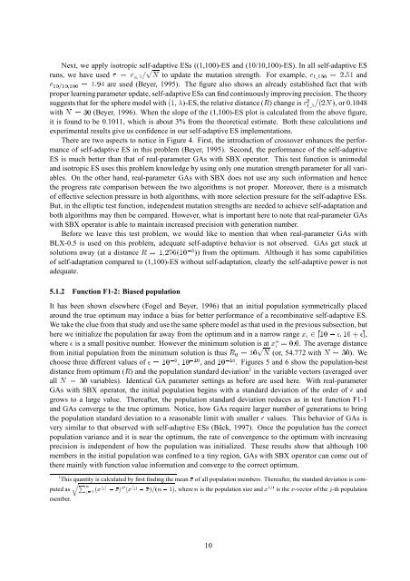
Next, we apply isotropic self-adaptive ESs ((1,100)-ES and (10/10,100)-ES). In all self-adaptive ES
runs, we have used=c;=pNto update the mutation strength. For example,c1;100=2:51and c10=10;100=1:94are used (Beyer, 1995). The figure also shows an already established fact that with
proper learning parameter update, self-adaptive ESs can find continuously improving precision. The theory
suggests that for the sphere model with(1;)-ES, the relative distance (R) change isc21;=(2N), or 0.1048
withN=30(Beyer, 1996). When the slope of the (1,100)-ES plot is calculated from the above figure,
it is found to be 0.1011, which is about 3% from the theoretical estimate. Both these calculations and
experimental results give us confidence in our self-adaptive ES implementations.
There are two aspects to notice in Figure 4. First, the introduction of crossover enhances the performance
of self-adaptive ES in this problem (Beyer, 1995). Second, the performance of the self-adaptive
ES is much better than that of real-parameter GAs with SBX operator. This test function is unimodal
and isotropic ES uses this problem knowledge by using only one mutation strength parameter for all variables.
On the other hand, real-parameter GAs with SBX does not use any such information and hence
the progress rate comparison between the two algorithms is not proper. Moreover, there is a mismatch
of effective selection pressure in both algorithms, with more selection pressure for the self-adaptive ESs.
But, in the elliptic test function, independent mutation strengths are needed to achieve self-adaptation and
both algorithms may then be compared. However, what is important here to note that real-parameter GAs
with SBX operator is able to maintain increased precision with generation number.
Before we leave this test problem, we would like to mention that when real-parameter GAs with
BLX-0.5 is used on this problem, adequate self-adaptive behavior is not observed. GAs get stuck at
solutions away (at a distanceR=1:276(10?5)) from the optimum. Although it has some capabilities
of self-adaptation compared to (1,100)-ES without self-adaptation, clearly the self-adaptive power is not
adequate.
5.1.2 Function F1-2: Biased population
It has been shown elsewhere (Fogel and Beyer, 1996) that an initial population symmetrically placed
around the true optimum may induce a bias for better performance of a recombinative self-adaptive ES.
We take the clue from that study and use the same sphere model as that used in the previous subsection, but
here we initialize the population far away from the optimum and in a narrow rangexi2[10?;10+],
where is a small positive number. However the minimum solution is atxi=0:0. The average distance
from initial population from the minimum solution is thusR0=10pN(or, 54.772 withN=30). We
choose three different values of=10?5,10?10, and10?15. Figures 5 and 6 show the population-best
distance from optimum (R) and the population standard deviation1 in the variable vectors (averaged over
allN=30variables). Identical GA parameter settings as before are used here. With real-parameter
GAs with SBX operator, the initial population begins with a standard deviation of the order of and
grows to a large value. Thereafter, the population standard deviation reduces as in test function F1-1
and GAs converge to the true optimum. Notice, how GAs require larger number of generations to bring
the population standard deviation to a reasonable limit with smaller values. This behavior of GAs is
very similar to that observed with self-adaptive ESs (Bäck, 1997). Once the population has the correct
population variance and it is near the optimum, the rate of convergence to the optimum with increasing
precision is independent of how the population was initialized. These results show that although 100
members in the initial population was confined to a tiny region, GAs with SBX operator can come out of
there mainly with function value information and converge to the correct optimum.
1
This quantity is calculated by first finding the meanxof all population members. Thereafter, the standard deviation is computed
asqPnj=1(x(j)?x)T(x(j)?x)=(n?1), wherenis the population size andx(j)is thex-vector of thej-th population
member.
10