Self-Adaptive Genetic Algorithms with Simulated Binary Crossover

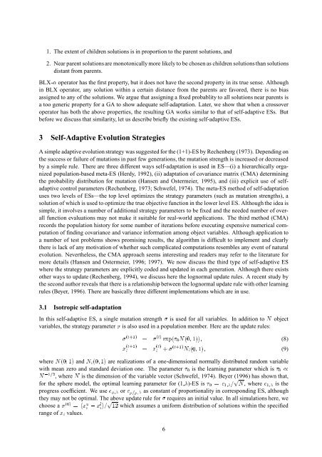
1. The extent of children solutions is in proportion to the parent solutions, and
2. Near parent solutions are monotonically more likely to be chosen as children solutions than solutions
distant from parents.
BLX- operator has the first property, but it does not have the second property in its true sense. Although
in BLX operator, any solution within a certain distance from the parents are favored, there is no bias
assigned to any of the solutions. We argue that assigning a fixed probablity to all solutions near parents is
a too generic property for a GA to show adequate self-adaptation. Later, we show that when a crossover
operator has both the above properties, the resulting GA works similar to that of self-adaptive ESs. But
before we discuss that similarity, let us describe briefly the existing self-adaptive ESs.
3 Self-Adaptive Evolution Strategies
A simple adaptive evolution strategy was suggested for the (1+1)-ES by Rechenberg (1973). Depending on
the success or failure of mutations in past few generations, the mutation strength is increased or decreased
by a simple rule. There are three different ways self-adaptation is used in ES—(i) a hierarchically organized
population-based meta-ES (Herdy, 1992), (ii) adaptation of covariance matrix (CMA) determining
the probability distribution for mutation (Hansen and Ostermeier, 1995), and (iii) explicit use of selfadaptive
control parameters (Rechenberg, 1973; Schwefel, 1974). The meta-ES method of self-adaptation
uses two levels of ESs—the top level optimizes the strategy parameters (such as mutation strengths), a
solution of which is used to optimize the true objective function in the lower level ES. Although the idea is
simple, it involves a number of additional strategy parameters to be fixed and the needed number of overall
function evaluations may not make it suitable for real-world applications. The third method (CMA)
records the population history for some number of iterations before executing expensive numerical computation
of finding covariance and variance information among object variables. Although application to
a number of test problems shows promising results, the algorithm is difficult to implement and clearly
there is lack of any motivation of whether such complicated computations resembles any event of natural
x(t+1)
evolution. Nevertheless, the CMA approach
i=x(t) (t+1)=(t)exp(0N(0;1));
seems
i+(t+1)Ni(0;1);
interesting and readers may refer to the literature for
more details (Hansen and Ostermeier, 1996; 1997). We now discuss the third type of self-adaptive ES
where the strategy parameters are explicitly coded and updated in each generation. Although there
is0/
exists
other ways to update (Rechenberg, 1994), we discuss here the lognormal update rules. A recent study by
the second author reveals that there is a relationship between the lognormal update rule with other learning
rules (Beyer, 1996). There are basically three different implementations which are in use.
3.1 Isotropic self-adaptation
In this self-adaptive ES, a single mutation strength is used for all variables. In addition toNobject
variables, the strategy parameter is also used in a population member. Here are the update rules:
(8)
(9)
whereN(0;1)andNi(0;1)are realizations of a one-dimensional normally distributed random variable
with mean zero and standard deviation one. The parameter0is the learning parameter which N?1=2, whereNis the dimension of the variable vector (Schwefel, 1974). Beyer (1996) has shown that,
for the sphere model, the optimal learning parameter for (1, )-ES is0=c1;=pN, wherec1;is the
progress coefficient. We usec;orc=;as constant of proportionality in corresponding ES, although
they may not be optimal. The above update rule for requires an initial value. In all simulations here, we
choose a(0)=(xui?xli)=p12which assumes a uniform distribution of solutions within the specified
range ofxivalues.
6