Self-Adaptive Genetic Algorithms with Simulated Binary Crossover
Self-Adaptive Genetic Algorithms with Simulated Binary Crossover
Self-Adaptive Genetic Algorithms with Simulated Binary Crossover

You also want an ePaper? Increase the reach of your titles
YUMPU automatically turns print PDFs into web optimized ePapers that Google loves.
Population standard deviation in x values<br />
1<br />
1e-10<br />
1e-20<br />
1st variable<br />
SBX<br />
30th variable<br />
15th variable<br />
1e-30<br />
1e-30<br />
1e-40<br />
1e-40<br />
0 500 1000<br />
F2-4:MinimizeNXi=1ix2i+10(1?cos(xi):<br />
1500 2000<br />
0 500 1000 1500 2000<br />
Generation Number<br />
Generation Number<br />
Figure 12: Mutation strengths for variables x1,x15, andx30are shown <strong>with</strong> self-adaptive<br />
(10/10,100)-ES for the function F2-1.<br />
(22)<br />
Figure 11: Population standard deviation in variablesx1,x15,<br />
andx30are shown <strong>with</strong> realparameter<br />
GAs <strong>with</strong> the SBX operator for the<br />
function F2-1.<br />
Mutation strengths for variables<br />
1<br />
1e-10<br />
1e-20<br />
1st variable<br />
(10/10,100)-ES<br />
30th variable<br />
15th variable<br />
Figure 15 shows that the (10/10,100)-ES <strong>with</strong> self-adaptation is able to converge near the optimum. The<br />
same is true <strong>with</strong> real-parameter GAs <strong>with</strong> SBX, but the rate of convergence is smaller compared to that<br />
of the self-adaptive ES.<br />
We now construct a multi-modal test function by adding a cosine term as follows:<br />
MinimizeNXi=10@iXj=1xj1A2:<br />
Figure 16 shows the performance of real-parameter GAs and self-adaptive ESs <strong>with</strong> identical parameter<br />
setting as on the elliptic function F2-3. Now, self-adaptive ES seems not able to converge to the global<br />
attractor (allxi=0having function value equal to zero), for the same reason as that described in section<br />
5.1.4—the initial mutation strength being too large to keep the population <strong>with</strong>in the global basin.<br />
When all initial mutation strengths reduced to one-tenth of their original values, non-isotropic ESs had no<br />
trouble in finding the true optimum <strong>with</strong> increased precision. We observe no such difficulty in GAs <strong>with</strong><br />
SBX operator and a performance similar to that in Function F2-3 is observed here.<br />
5.3 Correlated function<br />
Next, we consider a function where pair-wise interactions of variables exist. The following Schwefel’s<br />
function is chosen:<br />
F3-1: (23)<br />
The population is initialized atxi2[?1:0;1:0]. Figure 17 shows the performance of real-parameter GAs<br />
<strong>with</strong> SBX (=1) and tournament size 3, non-isotropic (4,100)-ES, and correlated (4,100)-ES. Although<br />
all methods have been able to find increased precision in obtained solutions, the rate of progress for the<br />
real-parameter GAs <strong>with</strong> SBX is slower compared to that of the correlated self-adaptive ESs. However,<br />
GAs <strong>with</strong> SBX makes a steady progress towards the optimum and performs better than the non-isotropic<br />
(4,100)-ES. The reason for the slow progress of real-parameter GAs is as follows. In the SBX operator,<br />
variable-by-variable crossover is used <strong>with</strong> a probability of 0.5. Correlations (or linkage) among the variables<br />
are not explicitly considered in this version of SBX. Although some such information comes via<br />
the population diversity in variables, it is not enough to progress faster towards the optimum in this problem<br />
compared to the correlated ES, where pairwise interactions among variables are explicitly considered.<br />
15