Hyperelliptic Curves, Continued Fractions and Somos Sequences

Hyperelliptic Curves, Continued Fractions 

and Somos Sequences 

Alf van der Poorten 

ceNTRe for Number Theory Research, Sydney 

May 8, 2007 Algorithmic Number Theory, Turku 

1

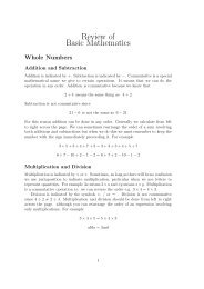
A pseudo-elliptic integral 

Z x 6t 

p t 4 + 4t 3 − 6t 2 + 4t + 1 dt 

Two Surprising Allegations 

“ 

= log x 6 + 12x 5 + 45x 4 + 44x 3 − 33x 2 + 43 

+(x 4 + 10x 3 + 30x 2 p 

+ 22x − 11) 

A Somos sequence of width 5 

x 4 + 4x 3 − 6x 2 + 4x + 1 

The sequence (Bh)−∞


Z x 6t 

p t 4 + 4t 3 − 6t 2 + 4t + 1 dt 


“ 

= log x 6 + 12x 5 + 45x 4 + 44x 3 − 33x 2 + 43 

+(x 4 + 10x 3 + 30x 2 p 

+ 22x − 11) 


x 4 + 4x 3 − 6x 2 + 4x + 1 



Z x 6t 

p t 4 + 4t 3 − 6t 2 + 4t + 1 dt 


“ 

= log x 6 + 12x 5 + 45x 4 + 44x 3 − 33x 2 + 43 

+(x 4 + 10x 3 + 30x 2 p 

+ 22x − 11) 


x 4 + 4x 3 − 6x 2 + 4x + 1 



Z x 6t 

p t 4 + 4t 3 − 6t 2 + 4t + 1 dt 


“ 

= log x 6 + 12x 5 + 45x 4 + 44x 3 − 33x 2 + 43 

+(x 4 + 10x 3 + 30x 2 p 

+ 22x − 11) 


x 4 + 4x 3 − 6x 2 + 4x + 1 



Z x 6t 

p t 4 + 4t 3 − 6t 2 + 4t + 1 dt 


“ 

= log x 6 + 12x 5 + 45x 4 + 44x 3 − 33x 2 + 43 

+(x 4 + 10x 3 + 30x 2 p 

+ 22x − 11) 


x 4 + 4x 3 − 6x 2 + 4x + 1 



Z x 6t 

p t 4 + 4t 3 − 6t 2 + 4t + 1 dt 


“ 

= log x 6 + 12x 5 + 45x 4 + 44x 3 − 33x 2 + 43 

+(x 4 + 10x 3 + 30x 2 p 

+ 22x − 11) 


x 4 + 4x 3 − 6x 2 + 4x + 1 


Michael Somos’s Sequences 

The story: Some fifteen years ago, Michael Somos noticed that the 

two-sided sequence Ch−2Ch+2 = Ch−1Ch+1 + C2 h , which I refer to as 

4-Somos in his honour, apparently takes only integer values if we start 

from C−1 , C0 , C1 , C2 = 1. 

Indeed, Somos goes on to investigate also the width 5 sequence, 

Bh−2Bh+3 = Bh−1Bh+2 + BhBh+1 , now with five initial 1s, the width 6 

sequence Dh−3Dh+3 = Dh−2Dh+2 + Dh−1Dh+1 + D2 h , and so on, testing 

whether each — when initiated by an appropriate number of 1s — 

yields only integers. Naturally, he asks: “What is going on here?" 

By the way, while 4-Somos (A006720), 5-Somos (A006721), 6-Somos 

(A006722), and 7-Somos (A006723), do yield only integers; 8-Somos 

does not. The codes in parentheses refer to Neil Sloane’s On-line 

encyclopedia of integer sequences. 

The reality: Somos actually first noticed that 6-Somos produces only 

integers while studying θ-function relations; he was subsequently 

reminded by others that the 4-analogue was known . . . . 

3





from C−1 , C0 , C1 , C2 = 1. 













3





from C−1 , C0 , C1 , C2 = 1. 













3





from C−1 , C0 , C1 , C2 = 1. 













3





from C−1 , C0 , C1 , C2 = 1. 













3





from C−1 , C0 , C1 , C2 = 1. 













3





from C−1 , C0 , C1 , C2 = 1. 













3





from C−1 , C0 , C1 , C2 = 1. 













3





from C−1 , C0 , C1 , C2 = 1. 













3

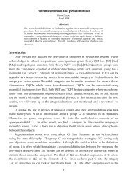
Concerning (Bh) — thus 5-Somos — Don Zagier inter alia writes: 

“One computes the first few (in my case, 300) terms Bn numerically, 

studies their numerical growth, and tries to fit this data by a nice 

analytic expression. One quickly finds that the growth is roughly 

exponential in n2 , but with some slow fluctuations around this and also 

with a dependency on the parity of n. This suggests trying the Ansatz 

Bn = c±bnan2 , where (−1) n = ±1. This is easily seen to give a 

solution to our recursion if a is the root of a12 = a4 + 1, and the 

numerical value a = 1.07283 (approx) does indeed give a reasonably 

good fit to the data, but eventually fails more and more thoroughly. 

Looking more carefully, we try the same Ansatz but with c± replaced by 

a function c±(n) which lies between fixed limits but is almost periodic 

in n, and this works, but with a new value a = 1.07425 (approx) . . . . 

Here I put in a pause so that we can catch our breath. 

Expanding the function c±(n) numerically into a Fourier series, we 

discover that it is a Jacobi theta function, and since theta functions (or 

quotients of them) are elliptic functions, this leads quickly to elliptic 

curves . . . .” 

4


















curves . . . .” 

4


















curves . . . .” 

4


















curves . . . .” 

4


















curves . . . .” 

4


















curves . . . .” 

4


















curves . . . .” 

4


















curves . . . .” 

4

The surprising integral 

Z X 6t dt 

p 

t4 + 4t3 − 6t2 + 4t + 1 

“ 

= log X 6 + 12X 5 + 45X 4 + 44X 3 − 33X 2 + 43 

+ (X 4 + 10X 3 + 30X 2 p 

+ 22X − 11) X 4 + 4X 3 − 6X 2 ” 

+ 4X + 1 

is a nice example of a class of pseudo-elliptic integrals 

Z X f (t)dt 

p = log 

D(t) ` q 

a(X) + b(X) D(X) ´ . (∗) 

Here we take D to be a monic polynomial defined over Q, of even 

degree 2g + 2, and not the square of a polynomial; f , a, and b denote 

appropriate polynomials. We suppose a to be nonzero, say of degree 

m at least g + 1. We will see that necessarily deg f = g , that 

deg b = m − g − 1, and that f has leading coefficient m. 

In the example, m = 6 and g = 1. 

5


Z X 6t dt 

p 

t4 + 4t3 − 6t2 + 4t + 1 

“ 

= log X 6 + 12X 5 + 45X 4 + 44X 3 − 33X 2 + 43 

+ (X 4 + 10X 3 + 30X 2 p 

+ 22X − 11) X 4 + 4X 3 − 6X 2 ” 

+ 4X + 1 


Z X f (t)dt 

p = log 

D(t) ` q 

a(X) + b(X) D(X) ´ . (∗) 







5


Z X 6t dt 

p 

t4 + 4t3 − 6t2 + 4t + 1 

“ 

= log X 6 + 12X 5 + 45X 4 + 44X 3 − 33X 2 + 43 

+ (X 4 + 10X 3 + 30X 2 p 

+ 22X − 11) X 4 + 4X 3 − 6X 2 ” 

+ 4X + 1 


Z X f (t)dt 

p = log 

D(t) ` q 

a(X) + b(X) D(X) ´ . (∗) 







5


Z X 6t dt 

p 

t4 + 4t3 − 6t2 + 4t + 1 

“ 

= log X 6 + 12X 5 + 45X 4 + 44X 3 − 33X 2 + 43 

+ (X 4 + 10X 3 + 30X 2 p 

+ 22X − 11) X 4 + 4X 3 − 6X 2 ” 

+ 4X + 1 


Z X f (t)dt 

p = log 

D(t) ` q 

a(X) + b(X) D(X) ´ . (∗) 







5


Z X 6t dt 

p 

t4 + 4t3 − 6t2 + 4t + 1 

“ 

= log X 6 + 12X 5 + 45X 4 + 44X 3 − 33X 2 + 43 

+ (X 4 + 10X 3 + 30X 2 p 

+ 22X − 11) X 4 + 4X 3 − 6X 2 ” 

+ 4X + 1 


Z X f (t)dt 

p = log 

D(t) ` q 

a(X) + b(X) D(X) ´ . (∗) 







5

Plainly, the equations detailing pseudo-elliptic integrals are purely 

formal and must therefore remain true with √ D replaced by its 

conjugate − √ D . Adding the two conjugate identities we see that 

Z 

0 dt = log ` a 2 − Db 2´ . (†) 

Thus a 2 − Db 2 is some constant k , and must be nonzero because D 

is not a square. In other words, u = a + b √ D is a nontrivial unit in the 

function field Q(X, p D(X)); and it is immediate that deg a = m 

implies deg b = m − g − 1. 

Differentiating uu yields 2aa ′ − 2bb ′ D − b 2 D ′ = 0. Hence b ˛ ˛aa ′ , and 

since a and b must be relatively prime because u is a unit, it follows 

that b ˛ ˛a ′ . Set f = a ′ /b, noting that indeed deg f = g and that f has 

leading coefficient m because a and b must have the same leading 

coefficient ∗ . 

∗ That common coefficient is 1 without loss of generality since we may freely 

choose the constant produced by the indefinite integration. 

6




Z 

0 dt = log ` a 2 − Db 2´ . (†) 












6




Z 

0 dt = log ` a 2 − Db 2´ . (†) 












6




Z 

0 dt = log ` a 2 − Db 2´ . (†) 












6




Z 

0 dt = log ` a 2 − Db 2´ . (†) 












6




Z 

0 dt = log ` a 2 − Db 2´ . (†) 












6




Z 

0 dt = log ` a 2 − Db 2´ . (†) 












6




Z 

0 dt = log ` a 2 − Db 2´ . (†) 












6




Z 

0 dt = log ` a 2 − Db 2´ . (†) 












6




Z 

0 dt = log ` a 2 − Db 2´ . (†) 












6




Z 

0 dt = log ` a 2 − Db 2´ . (†) 












6




Z 

0 dt = log ` a 2 − Db 2´ . (†) 












6

Moreover, 

u ′ = a ′ + b ′√ D + bD ′ /2 √ D 

= a ′ + (2bb ′ D + b 2 D ′ )/2b √ D = a ′ + aa ′ /b √ D . 

So, remarkably, u ′ = f (b √ D + a)/ √ D = fu/ √ D . 

Thus, to verify the evaluation of the pseudo-elliptic integral it suffices to 

make the not altogether obvious substitution u(x) = a + b √ D . Of 

course the real question is how to guess the polynomials a and b. 

Remark. The case g = 0, say D(X) = X 2 + 2vX + w , is useful for 

orienting oneself. Here (X + v) + p D(X) is a unit, of norm v 2 − w , 

and indeed 

Z 

dX 

√ X 2 + 2vX + w 

= sinh −1 

X + v 

p 

w − v 2 = log` p 

X + v + X 2 + 2vX + w ´ . 

Notice that deg f = 0 and has leading coefficient 1, as predicted. 

7

Moreover, 

u ′ = a ′ + b ′√ D + bD ′ /2 √ D 









Z 

dX 

√ X 2 + 2vX + w 

= sinh −1 

X + v 

p 

w − v 2 = log` p 

X + v + X 2 + 2vX + w ´ . 


7

Moreover, 

u ′ = a ′ + b ′√ D + bD ′ /2 √ D 









Z 

dX 

√ X 2 + 2vX + w 

= sinh −1 

X + v 

p 

w − v 2 = log` p 

X + v + X 2 + 2vX + w ´ . 


7

Moreover, 

u ′ = a ′ + b ′√ D + bD ′ /2 √ D 









Z 

dX 

√ X 2 + 2vX + w 

= sinh −1 

X + v 

p 

w − v 2 = log` p 

X + v + X 2 + 2vX + w ´ . 


7

Moreover, 

u ′ = a ′ + b ′√ D + bD ′ /2 √ D 









Z 

dX 

√ X 2 + 2vX + w 

= sinh −1 

X + v 

p 

w − v 2 = log` p 

X + v + X 2 + 2vX + w ´ . 


7

Moreover, 

u ′ = a ′ + b ′√ D + bD ′ /2 √ D 









Z 

dX 

√ X 2 + 2vX + w 

= sinh −1 

X + v 

p 

w − v 2 = log` p 

X + v + X 2 + 2vX + w ´ . 


7

Moreover, 

u ′ = a ′ + b ′√ D + bD ′ /2 √ D 









Z 

dX 

√ X 2 + 2vX + w 

= sinh −1 

X + v 

p 

w − v 2 = log` p 

X + v + X 2 + 2vX + w ´ . 


7

Moreover, 

u ′ = a ′ + b ′√ D + bD ′ /2 √ D 









Z 

dX 

√ X 2 + 2vX + w 

= sinh −1 

X + v 

p 

w − v 2 = log` p 

X + v + X 2 + 2vX + w ´ . 


7

Moreover, 

u ′ = a ′ + b ′√ D + bD ′ /2 √ D 









Z 

dX 

√ X 2 + 2vX + w 

= sinh −1 

X + v 

p 

w − v 2 = log` p 

X + v + X 2 + 2vX + w ´ . 


7

Moreover, 

u ′ = a ′ + b ′√ D + bD ′ /2 √ D 









Z 

dX 

√ X 2 + 2vX + w 

= sinh −1 

X + v 

p 

w − v 2 = log` p 

X + v + X 2 + 2vX + w ´ . 


7

Units and Torsion 

The notion unit entails that u be trivial at other than infinite places 

(absolute values). That is, the divisor of zeros and poles of the function 

u = a + b √ D is supported only at infinity. 

Plainly speaking, the quartic C : Y 2 = X 4 + 4X 3 − 6X 2 + 4X + 1 has 

two points at infinity, which I shall call S , and O — the latter being the 

zero of the group law on the elliptic curve C . In general, for 

C : Y 2 = D(X) of genus g , I am unfortunately forced to talk about the 

divisor at infinity on C , or worse, about its class as a point on the 

Jacobian of the hyperelliptic curve C . 

Whatever, whenever we meet a pseudo-elliptic integral, there is a 

positive integer m so that m(S − O) is the divisor of a unit u , showing 

that S − O provides a torsion point of order m on Jac(C). 

8














8














8














8














8














8














8














8

Units in Quadratic Fields and Continued Fractions 

One finds a unit u in the quadratic domain Q[X, Y ] by studying the 

continued fraction expansion of Y = p D(X). The principle is that a 

period of the expansion produces a unit and, conversely, the existence 

of a unit entails the periodicity of the continued fraction expansion. 

Thus — because periodicity is equivalent to torsion at infinity — each 

step in the continued fraction expansion of Y must somehow add 

some multiple of the divisor at infinity. This fact was nicely ‘explicited’ in 

the elliptic case by Bill Adams and Mike Razar (1981); there is a more 

recent analogous proof for general g by Tom Berry. 

It’s pretty obvious that torsion at infinity is unusual in characteristic zero. 

So periodicity of the expansion of Y must therefore be exceptional. 

In the numerical case, and for congruence function fields, periodicity is 

always forced by the box principle. But, over an infinite field, there are 

infinitely many polynomials of bounded degree . . . ; so periodicity is 

rare happenstance. 

9

















9

















9

















9

















9

















9

















9

















9

















9

















9

Continued Fraction of the Square Root of a Polynomial 

Set Y 2 = D(X) where D = is a monic polynomial of degree 2g + 2. 

Then we may write 

D(X) = ` A(X) ´ 2 + 4R(X) , 

where A is the polynomial part of the square root Y of D and 4R , with 

deg R ≤ g , is the remainder. We then take 

Y = A ` 1 + 4R/A 2´ 1/2 = A(X) + c1X −1 + c2X −2 + · · · 

thereby viewing Y as an element of K ((X −1 )), Laurent series in the 

variable 1/X . All this makes sense over any base field K not of 

characteristic 2. 

However, below I deal with the quadratic irrational function Z defined 

by 

C : Z 2 − AZ − R = 0 ; in effect Z = 1 

(Y + A). (‡) 

2 

Then deg Z = deg A = g + 1, while its conjugate satisfies deg Z < 0; 

so Z is reduced. Note that Z makes sense in arbitrary characteristic, 

including characteristic two. 

10




D(X) = ` A(X) ´ 2 + 4R(X) , 



Y = A ` 1 + 4R/A 2´ 1/2 = A(X) + c1X −1 + c2X −2 + · · · 





by 


(Y + A). (‡) 

2 




10




D(X) = ` A(X) ´ 2 + 4R(X) , 



Y = A ` 1 + 4R/A 2´ 1/2 = A(X) + c1X −1 + c2X −2 + · · · 





by 


(Y + A). (‡) 

2 




10




D(X) = ` A(X) ´ 2 + 4R(X) , 



Y = A ` 1 + 4R/A 2´ 1/2 = A(X) + c1X −1 + c2X −2 + · · · 





by 


(Y + A). (‡) 

2 




10




D(X) = ` A(X) ´ 2 + 4R(X) , 



Y = A ` 1 + 4R/A 2´ 1/2 = A(X) + c1X −1 + c2X −2 + · · · 





by 


(Y + A). (‡) 

2 




10




D(X) = ` A(X) ´ 2 + 4R(X) , 



Y = A ` 1 + 4R/A 2´ 1/2 = A(X) + c1X −1 + c2X −2 + · · · 





by 


(Y + A). (‡) 

2 




10




D(X) = ` A(X) ´ 2 + 4R(X) , 



Y = A ` 1 + 4R/A 2´ 1/2 = A(X) + c1X −1 + c2X −2 + · · · 





by 


(Y + A). (‡) 

2 




10




D(X) = ` A(X) ´ 2 + 4R(X) , 



Y = A ` 1 + 4R/A 2´ 1/2 = A(X) + c1X −1 + c2X −2 + · · · 





by 


(Y + A). (‡) 

2 




10




D(X) = ` A(X) ´ 2 + 4R(X) , 



Y = A ` 1 + 4R/A 2´ 1/2 = A(X) + c1X −1 + c2X −2 + · · · 





by 


(Y + A). (‡) 

2 




10

To detail the continued fraction expansion, for h ∈ Z set 

Zh = (Z + Ph)/Qh , 

where Ph and Qh are polynomials satisfying deg Ph ≤ g − 1, 

deg Qh ≤ g and Qh divides the norm (Z + Ph)(Z + Ph). 

Insist that deg Z0 > 0 and deg Z 0 < 0. Then, deg Zh > 0 and 

deg Z h < 0 — that is, the Zh all are reduced — and the K [X]-module 

〈Qh, Z + Ph〉 is in fact an ideal of the domain K [X, Z ]. 

Finally, denote by ah the polynomial part of Zh . Then the continued 

fraction expansion of say Z0 is a tableau of lines (or steps) 

(Z + Ph)/Qh = ah − (Z + Ph+1)/Qh in brief: Zh = ah − R−h , 

where, −Qh/(Z + Ph+1) = (Z + Ph+1)/Qh+1 . Necessarily 

Ph + Ph+1 + A = ahQh and (Z + Ph+1)(Z + Ph+1) = −QhQh+1 , 

and one easily verifies that the conditions on the Ph and Qh are 

sustained. 

11


Zh = (Z + Ph)/Qh , 












sustained. 

11


Zh = (Z + Ph)/Qh , 












sustained. 

11


Zh = (Z + Ph)/Qh , 












sustained. 

11


Zh = (Z + Ph)/Qh , 












sustained. 

11


Zh = (Z + Ph)/Qh , 












sustained. 

11


Zh = (Z + Ph)/Qh , 












sustained. 

11


Zh = (Z + Ph)/Qh , 












sustained. 

11

There is a minor miracle. Because the complete quotients Zh all are 

reduced it follows that also all the ‘remainders’ R−h are reduced. Thus 

the partial quotients ah , which begin life as the polynomial parts of the 

Zh , also are the polynomial parts of the R−h . 

Thus also the conjugate line 

R−h = (Z + Ph+1)/Qh = ah − (Z + Ph)/Qh = ah − Z h 

is a line in an admissible continued fraction expansion, explaining why I 

can refer to the original expansion as bi-directional infinite. 

When the base field K is infinite (say K = Q), I assert that a generic 

choice of P0 and Q0 is so that all the ah are linear — equivalently, so 

that all the Qh are of degree g — indeed, a teeny bit less obviously, so 

that all the Ph are of their maximal degree g − 1. 

That’s so because the probability of an element of K being zero — is 

zero. 

It is the same thing to note that a generic divisor of C is defined by a 

g -tuple of elements of an algebraic extension of K . 

12














zero. 



12














zero. 



12














zero. 



12














zero. 



12














zero. 



12














zero. 



12














zero. 



12














zero. 



12














zero. 



12

I should point out that any actual expansion is very messy. I give the list 

of partial quotients of two very different examples. First 

p 

X 4 − 2X 3 + 3X 2 + 2X + 1 + (X 2 − X + 1) = 

[2(X 2 − X + 1) , 1 2 X − 1 2 , 2X − 2 , 1 2 X 2 − 1 2 X + 1 2 , 2X − 2 , 1 2 X − 1 2 ]. 

Here, I’ve copied the expansion of 2Z in a periodic case (so, there’s a 

pseudo-elliptic integral with D = X 4 − 2X 3 + 3X 2 + 2X + 1). Note that 

the quasi-period already supplies a unit. In fact 

Z X 4t − 1 

p t 4 − 2t 3 + 3t 2 + 2t + 1 dt = 

log ` X 4 −3X 3 +5X 2 −2X 

+(X 2 p 

− 2X + 2) X 4 − 2X 3 + 3X 2 + 2X + 1 ´ . 

13



p 

X 4 − 2X 3 + 3X 2 + 2X + 1 + (X 2 − X + 1) = 

[2(X 2 − X + 1) , 1 2 X − 1 2 , 2X − 2 , 1 2 X 2 − 1 2 X + 1 2 , 2X − 2 , 1 2 X − 1 2 ]. 




Z X 4t − 1 

p t 4 − 2t 3 + 3t 2 + 2t + 1 dt = 

log ` X 4 −3X 3 +5X 2 −2X 

+(X 2 p 

− 2X + 2) X 4 − 2X 3 + 3X 2 + 2X + 1 ´ . 

13



p 

X 4 − 2X 3 + 3X 2 + 2X + 1 + (X 2 − X + 1) = 

[2(X 2 − X + 1) , 1 2 X − 1 2 , 2X − 2 , 1 2 X 2 − 1 2 X + 1 2 , 2X − 2 , 1 2 X − 1 2 ]. 




Z X 4t − 1 

p t 4 − 2t 3 + 3t 2 + 2t + 1 dt = 

log ` X 4 −3X 3 +5X 2 −2X 

+(X 2 p 

− 2X + 2) X 4 − 2X 3 + 3X 2 + 2X + 1 ´ . 

13



p 

X 4 − 2X 3 + 3X 2 + 2X + 1 + (X 2 − X + 1) = 

[2(X 2 − X + 1) , 1 2 X − 1 2 , 2X − 2 , 1 2 X 2 − 1 2 X + 1 2 , 2X − 2 , 1 2 X − 1 2 ]. 




Z X 4t − 1 

p t 4 − 2t 3 + 3t 2 + 2t + 1 dt = 

log ` X 4 −3X 3 +5X 2 −2X 

+(X 2 p 

− 2X + 2) X 4 − 2X 3 + 3X 2 + 2X + 1 ´ . 

13



p 

X 4 − 2X 3 + 3X 2 + 2X + 1 + (X 2 − X + 1) = 

[2(X 2 − X + 1) , 1 2 X − 1 2 , 2X − 2 , 1 2 X 2 − 1 2 X + 1 2 , 2X − 2 , 1 2 X − 1 2 ]. 




Z X 4t − 1 

p t 4 − 2t 3 + 3t 2 + 2t + 1 dt = 

log ` X 4 −3X 3 +5X 2 −2X 

+(X 2 p 

− 2X + 2) X 4 − 2X 3 + 3X 2 + 2X + 1 ´ . 

13

Second, if we replace D by D + 1 then we obtain a generic expansion 

nicely illustrating the behaviour of Néron–Tate height. 

p 

X 4 − 2X 3 + 3X 2 + 2X + 2 + (X 2 − X + 1) 

= [2(X 2 − X + 1) , 1 2 X − 5 8 

− 488095744 X + 16216931891200 

2572789149 34035427652121 

− 1600956438806866952192000 

88607770352600487715818861 

, 32X 

− 344 

21 441 

, − 21440698686186129 

1136033082245120 

, − 9261X 

− 2963079 

7936 1968128 , 

X + 1665322334299891329867 

42646681907481804800 , 

X − 3371996766956576002150497085030400 

256351315939101539512201711796263641 , 

80083198356049188999341382795525473293961 

975968207083235989098500587163484160000 X 

− 255369300674062782420731816474523944637364177546099 

12679074228671726095323776878469612834847195136000 , 

4117934429867578468642904208184426566140181398969531760640000 

503230723831903952989142036290969243284756393383295955214733129X − 267842912006437191134169045543528305515206296540594830431118591703121920000 , . . . . . .] 

22953474733170075135048388320813442171721920531699498816628220662260670805921 

Even a computer chokes on numbers growing at such a pace. 

14



p 

X 4 − 2X 3 + 3X 2 + 2X + 2 + (X 2 − X + 1) 

= [2(X 2 − X + 1) , 1 2 X − 5 8 

− 488095744 X + 16216931891200 

2572789149 34035427652121 

− 1600956438806866952192000 

88607770352600487715818861 

, 32X 

− 344 

21 441 

, − 21440698686186129 

1136033082245120 

, − 9261X 

− 2963079 

7936 1968128 , 

X + 1665322334299891329867 

42646681907481804800 , 

X − 3371996766956576002150497085030400 

256351315939101539512201711796263641 , 

80083198356049188999341382795525473293961 

975968207083235989098500587163484160000 X 

− 255369300674062782420731816474523944637364177546099 

12679074228671726095323776878469612834847195136000 , 

4117934429867578468642904208184426566140181398969531760640000 

503230723831903952989142036290969243284756393383295955214733129X − 267842912006437191134169045543528305515206296540594830431118591703121920000 , . . . . . .] 

22953474733170075135048388320813442171721920531699498816628220662260670805921 


14



p 

X 4 − 2X 3 + 3X 2 + 2X + 2 + (X 2 − X + 1) 

= [2(X 2 − X + 1) , 1 2 X − 5 8 

− 488095744 X + 16216931891200 

2572789149 34035427652121 

− 1600956438806866952192000 

88607770352600487715818861 

, 32X 

− 344 

21 441 

, − 21440698686186129 

1136033082245120 

, − 9261X 

− 2963079 

7936 1968128 , 

X + 1665322334299891329867 

42646681907481804800 , 

X − 3371996766956576002150497085030400 

256351315939101539512201711796263641 , 

80083198356049188999341382795525473293961 

975968207083235989098500587163484160000 X 

− 255369300674062782420731816474523944637364177546099 

12679074228671726095323776878469612834847195136000 , 

4117934429867578468642904208184426566140181398969531760640000 

503230723831903952989142036290969243284756393383295955214733129X − 267842912006437191134169045543528305515206296540594830431118591703121920000 , . . . . . .] 

22953474733170075135048388320813442171721920531699498816628220662260670805921 


14



p 

X 4 − 2X 3 + 3X 2 + 2X + 2 + (X 2 − X + 1) 

= [2(X 2 − X + 1) , 1 2 X − 5 8 

− 488095744 X + 16216931891200 

2572789149 34035427652121 

− 1600956438806866952192000 

88607770352600487715818861 

, 32X 

− 344 

21 441 

, − 21440698686186129 

1136033082245120 

, − 9261X 

− 2963079 

7936 1968128 , 

X + 1665322334299891329867 

42646681907481804800 , 

X − 3371996766956576002150497085030400 

256351315939101539512201711796263641 , 

80083198356049188999341382795525473293961 

975968207083235989098500587163484160000 X 

− 255369300674062782420731816474523944637364177546099 

12679074228671726095323776878469612834847195136000 , 

4117934429867578468642904208184426566140181398969531760640000 

503230723831903952989142036290969243284756393383295955214733129X − 267842912006437191134169045543528305515206296540594830431118591703121920000 , . . . . . .] 

22953474733170075135048388320813442171721920531699498816628220662260670805921 


14

In the course of studying continued fraction expansions 

(Z + Ph)/Qh = ah − (Z + Ph+1)/Qh , h ∈ Z 

in quadratic function fields I learned that the leading coefficients, say 

dh , of the polynomials Ph control the degeneracies of the expansion. 

So I chose to try to describe the other parameters detailing the Ph and 

Qh in terms of the dh . 

Denote a typical zero of Qh by ϑh and recall the recursion relations 

Ph + Ph+1 + A = ahQh and 

− QhQh+1 = (Z + Ph+1)(Z + Ph+1) = −R + Ph+1(A + Ph+1) . 

Thus Ph(ϑh) + Ph+1(ϑh) + A(ϑh) = 0, R(ϑh) = −Ph+1(ϑh)Ph(ϑh). 

Hence Qh(X) divides R(X) + Ph+1(X)Ph(X), and so 

Ch(X)/uh = ` R(X) + Ph+1(X)Ph(X) ´ /Qh(X) 

defines a polynomial Ch . Here uh is the leading coefficient of Qh . 

It’s useful that deg Ch = max ` g, 2(g − 1) ´ − g ; so Ch is a constant if 

g = 1 or g = 2. 

15















g = 1 or g = 2. 

15















g = 1 or g = 2. 

15















g = 1 or g = 2. 

15















g = 1 or g = 2. 

15

What the Continued Fraction Does 

Note that (Z + Ph)(Z + Ph) = −R + APh + P 2 h . Suppose ϑh denotes a 

typical zero of Qh . Then the condition: Qh divides the norm 

(Z + Ph)(Z + Ph) asserts that R(ϑh) = ` A(ϑh) + Ph(ϑh) ´ Ph(ϑh). 

However, recall that Z defines the hyperelliptic curve 

C : Z 2 − AZ − R = 0 

of genus g . Of course C is defined over K but, for a moment 

disregarding that, it follows from the remarks above that the point 

` ϑh, −Ph(ϑh) ´ is a point on C . In general deg Qh = g and so has g 

conjugate zeros. That gives a g -tuple of conjugate points on C , or in 

proper language, a divisor defined over K on C . 

As we have already seen, the consecutive divisor classes differ by 

some multiple (in fact the degree of ah ) of the class of the divisor S at 

infinity on (the Jacobian) of C . If deg ah = 1 for all h this provides a 

sequence (Mh) of divisors, with Mh = M + hS . 

If g = 1, C is an elliptic curve equal to its Jacobian; and the story is 

about honest-to-goodness points on the curve. 

16






C : Z 2 − AZ − R = 0 












16






C : Z 2 − AZ − R = 0 












16






C : Z 2 − AZ − R = 0 












16






C : Z 2 − AZ − R = 0 












16






C : Z 2 − AZ − R = 0 












16






C : Z 2 − AZ − R = 0 












16

The elliptic case 

When g = 1 we have deg Ph = 0 and set Ph = dh , and deg Qh = 1, 

say with Qh(X) = uh(X − wh). Then deg A = 2 and set, say, 

R = u(X − w). 

Happily, the birational transformation U = Z , V − u = XZ , transforms 

our quartic curve into a cubic model passing through the origin 

E : V 2 − uV = monic cubic in U with zero constant term; 

the points (wh, −dh) on C become (−dh, u − whdh) on E . The point S 

is now (0, 0). It is then easy to use the continued fraction recursion 

formulæ to verify explicitly that Sh = hS . 

We have −R(wh) = dhdh+1 , Ch = u , and −Ch−1ChQh−1(w)Qh(w) is 

both u 2 Ph(w) ` A(w) + Ph(w) ´ and −uh−1uhdh−1d 2 h dh+1 . Thus 

dh−1d 2 h dh+1 = u 2` dh + A(w) ´ ; 

a recursion involving the dh only. But, the dh are very messy . . . . 

17




R = u(X − w). 









dh−1d 2 h dh+1 = u 2` dh + A(w) ´ ; 


17




R = u(X − w). 









dh−1d 2 h dh+1 = u 2` dh + A(w) ´ ; 


17




R = u(X − w). 









dh−1d 2 h dh+1 = u 2` dh + A(w) ´ ; 


17




R = u(X − w). 









dh−1d 2 h dh+1 = u 2` dh + A(w) ´ ; 


17




R = u(X − w). 









dh−1d 2 h dh+1 = u 2` dh + A(w) ´ ; 


17




R = u(X − w). 









dh−1d 2 h dh+1 = u 2` dh + A(w) ´ ; 


17




R = u(X − w). 









dh−1d 2 h dh+1 = u 2` dh + A(w) ´ ; 


17




R = u(X − w). 









dh−1d 2 h dh+1 = u 2` dh + A(w) ´ ; 


17




R = u(X − w). 









dh−1d 2 h dh+1 = u 2` dh + A(w) ´ ; 


17




R = u(X − w). 









dh−1d 2 h dh+1 = u 2` dh + A(w) ´ ; 


17

The −dh are in fact the abscissæ of points on E (specifically, of the 

points M + hS ); so they are rationals whose denominators A2 h , say, are 

squares of integers. Accordingly, define a sequence (Ah) by 

Ah−1Ah+1 = dhA 2 h . 

Conveniently, this immediately yields Ah−2Ah+2 = dh−1d 2 h dh+1A 2 h . 

So dh−1d 2 h dh+1 = u 2` dh + A(w) ´ is 

Ah−2Ah+2 = u 2 Ah−1Ah+1 + u 2 A(w)A 2 h , 

showing that all Somos 4 sequences come from (at most quadratic 

twists of) rational elliptic curves. 

A careful look (for example: Rachel Shipsey’s thesis) at the behaviour 

of points M + hS on an elliptic curve confirms that the Ah will all be 

S -integers — with the primes of the finite set S coming from the 

factors of the initial values A0 , A1 , A2 , A3 use and the denominators of 

the coefficients v and A(w) of the Somos relation. 

18




Ah−1Ah+1 = dhA 2 h . 











18




Ah−1Ah+1 = dhA 2 h . 











18




Ah−1Ah+1 = dhA 2 h . 











18




Ah−1Ah+1 = dhA 2 h . 











18




Ah−1Ah+1 = dhA 2 h . 











18




Ah−1Ah+1 = dhA 2 h . 











18




Ah−1Ah+1 = dhA 2 h . 











18

As it happens, a combinatorial/algebraic result, a corollary of Fomin 

and Zelevinsky’s theory of cluster algebras, guarantees that elements 

of Somos 4, . . . , Somos 7 sequences are Laurent polynomials in the 

initial values with coefficient ring polynomials in the coefficients of the 

defining recursion. 

Somos 5 sequences also come from elliptic curves. It’s not difficult to 

find that 

Ah−1Ah+2 = dhdh+1AhAh+1 . 

The ingenious observation that 

dh+1dh + u 2 /dh + dhdh−1 

is independent of h — that is, it is a discrete integral of the recursion for 

the dh — now readily yields an identity providing the width 5 recursion 

Ah−2Ah+3 = −u 2 A(w)Ah−1Ah+2 + u 3` u + 2wA(w) ´ AhAh+1. 

A Somos 5 may be a Somos 4. In any case, its two subsequences 

(A2h+1) and (A2h) are different Somos 4 sequences deriving from the 

one elliptic curve and the same addition by SE = (0, 0), but with initial 

translations ME differing by 1 

2 SE . 

19







find that 











2 SE . 

19







find that 











2 SE . 

19







find that 











2 SE . 

19







find that 











2 SE . 

19







find that 











2 SE . 

19







find that 











2 SE . 

19







find that 











2 SE . 

19







find that 











2 SE . 

19







find that 











2 SE . 

19

Elliptic Divisibility Sequences 

Now consider the singular case, M = S : thus the expansion of Z . It 

will be convenient to write e in place of d , and — in honour of Morgan 

Ward — (Wh) in place of (Ah). A brief computation reveals a0(X) = A, 

e1 = 0, Q1(X) := u(X − w), e2 = −A(w), sufficing — using the 

recursion for the sequence (dh) — to set W1 = 1, W2 = u , leading to 

W3 = −u 2 A(w), W4 = −u 4` u + 2wA(w) ´ , . . . and one then notices 

that (Wh) supplies the coefficients in 

Ah−2Ah+2 = W 2 2 Ah−1Ah+1 − W1W3A 2 h . 

I realised much later that this was obvious and did not need any work. 

The point is that the recursion leading to the Ah is independent of the 

translation M . So, the coefficients above must be precisely those that 

fit the singular case Ah = Wh . I twigged to this self-determining 

principle after Kate Stange first showed me her work on elliptic nets; 

and then realised I had already used it in work with Chris Swart. 

20
















20
















20
















20
















20
















20
















20
















20
















20
















20
















20
















20
















20
















20
















20
















20

Remarkably, Ward introduces his sequence (Wh) in effect as satisfying 

W−h = −Wh and the multi-recursion 

W 2 n Wh−mWh+m = W 2 mWh−nWh+n − Wm−nWm+nW 2 h . 

Yet, the special case n = 1, m = 2, and the values W1 , W2 , W3 , W4 

already determine the sequence. 

Ward proves the coherence of his definition by showing there does 

exist a solution sequence defined in terms of Weierstrass σ -functions. 

Recently, Christine Swart and I re-explored this matter and found a 

direct proof that for all m and n 

W 2 n Ah−mAh+m = W 2 mAh−nAh+n − Wm−nWm+nA 2 h . 

Our argument relies on the amusingly symmetrical identity 

(dh−1 − em)d 2 h (dh+1 − em) = (em−1 − dh)e 2 m(em+1 − dh) . 

We have a similar argument and analogous result in the odd gap case. 

21














21














21














21














21














21

Elliptic Division Polynomials 

I insisted that the cubic model E of our elliptic curve contain (0, 0). 

However, we may suppose we had obtained our E = E(x, y) from a 

more general elliptic curve by translating a notional point S = (x, y) on 

it to the origin. Then the coefficients of E are polynomials in x and y , 

themselves with coefficients polynomials in the defining data. This 

makes the Wh polynomials in x and y . 

More, mS = 0 and Wm(a, b) = 0 if and only if S = (a, b) is a torsion 

point of order m on E . So the polynomial Wh(x, y) is the h-th division 

polynomial. That inter alia entails 

gcd ` Wr (x, y), Ws(x, y) ´ = W gcd(r,s)(x, y), 

explaining the division properties of the Wh(0, 0). 

˛ 

By the way, Rachel Shipsey proves directly that if W1 = 1 and W2 

˛W4 

then r ˛ ˛ 

˛s entails Wr ˛Ws ; hence again: elliptic divisibility sequence. 

22













˛ 


˛W4 

then r ˛ ˛ 


22













˛ 


˛W4 

then r ˛ ˛ 


22













˛ 


˛W4 

then r ˛ ˛ 


22













˛ 


˛W4 

then r ˛ ˛ 


22













˛ 


˛W4 

then r ˛ ˛ 


22













˛ 


˛W4 

then r ˛ ˛ 


22













˛ 


˛W4 

then r ˛ ˛ 


22

4-Somos 

Suppose (Ch) = (. . . , 2, 1, 1, 1, 1, 2, 3, 7, . . . ) with 

Ch−2Ch+2 = Ch−1Ch+1 + C2 h . My formulaire quickly reveals that 

u = ±1, w = ∓2, A(w) = 1, and thus that (Ch) arises from 

Z 2 − (X 2 − 3)Z − (X − 2) = 0 with M = (1, −1); 

equivalently from E : V 2 − V = U 3 + 3U 2 + 2U with ME = (−1, 1). 


The case (Bh) = (. . . , 2, 1, 1, 1, 1, 1, 2, 3, 5, 11, . . . ) with 

Bh−2Bh+3 = Bh−1Bh+2 + BhBh+1 is trickier. One needs to define 

chBh−1Bh+1 = ehB 2 h with chch+1 independent of h. It turns out that 

(Bh) arises from 

Z 2 − (X 2 − 29)Z − 48(X + 5) = 0 with M = (−3, −10); 

equivalently from E : V 2 + UV + 6V = U 3 + 7U 2 + 12U with 

ME = (−2, −2). The fact gcd(6, 12) = 1 is the difficulty preventing the 

sequence from being a Somos 4. 

By symmetry each respective M is a point of order 2 on its curve. 

23





Z 2 − (X 2 − 3)Z − (X − 2) = 0 with M = (1, −1); 







Z 2 − (X 2 − 29)Z − 48(X + 5) = 0 with M = (−3, −10); 





23





Z 2 − (X 2 − 3)Z − (X − 2) = 0 with M = (1, −1); 







Z 2 − (X 2 − 29)Z − 48(X + 5) = 0 with M = (−3, −10); 





23





Z 2 − (X 2 − 3)Z − (X − 2) = 0 with M = (1, −1); 







Z 2 − (X 2 − 29)Z − 48(X + 5) = 0 with M = (−3, −10); 





23





Z 2 − (X 2 − 3)Z − (X − 2) = 0 with M = (1, −1); 







Z 2 − (X 2 − 29)Z − 48(X + 5) = 0 with M = (−3, −10); 





23





Z 2 − (X 2 − 3)Z − (X − 2) = 0 with M = (1, −1); 







Z 2 − (X 2 − 29)Z − 48(X + 5) = 0 with M = (−3, −10); 





23





Z 2 − (X 2 − 3)Z − (X − 2) = 0 with M = (1, −1); 







Z 2 − (X 2 − 29)Z − 48(X + 5) = 0 with M = (−3, −10); 





23





Z 2 − (X 2 − 3)Z − (X − 2) = 0 with M = (1, −1); 







Z 2 − (X 2 − 29)Z − 48(X + 5) = 0 with M = (−3, −10); 





23





Z 2 − (X 2 − 3)Z − (X − 2) = 0 with M = (1, −1); 







Z 2 − (X 2 − 29)Z − 48(X + 5) = 0 with M = (−3, −10); 





23





Z 2 − (X 2 − 3)Z − (X − 2) = 0 with M = (1, −1); 







Z 2 − (X 2 − 29)Z − 48(X + 5) = 0 with M = (−3, −10); 





23





Z 2 − (X 2 − 3)Z − (X − 2) = 0 with M = (1, −1); 







Z 2 − (X 2 − 29)Z − 48(X + 5) = 0 with M = (−3, −10); 





23

Higher Genus 

There surely are analogous results for higher genus curves, particularly 

for hyperelliptic curves. Indeed, more than a dozen years ago, David 

Cantor showed for all hyperelliptic curves (of odd degree) that there are 

analogues of the division polynomials satisfying relations given by 

certain Kronecker–Hankel determinants. 

My continued fraction program falters almost immediately, though I can 

completely handle curves Z 2 − AZ − R = 0 with deg A = 3 provided 

that deg R = −v(X − W ) is linear. 

In that case, I find that 

dh−2d 2 h−1 d 3 h d 2 h+1 dh+2 = v 2 dh−1d 2 h dh+1 − v 3 A(w), 

yielding a width 6 relation 

Ah−3Ah+3 = v 2 Ah−2Ah+2 − v 3 A(w)A 2 h . 

24

Higher Genus 













24

Higher Genus 













24

Higher Genus 













24

Higher Genus 













24

Higher Genus 













24

Others can do worse, and better. If g = 1, Andy Hone notes that 

α = ℘ ′ (y) 2 , β = ℘ ′ (y) 2 (℘(2y) − ℘(y)) yields the identity 

` ℘(x + y) − ℘(y) ´` ℘(x) − ℘(y) ´ 2` ℘(x − y) − ℘(y) ´ 

= −α ` ℘(x) − ℘(y) ´ + β . 

This also is a remark of Nelson Stephens basic to Christine Swart’s 

thesis. Notice that it is precisely my relation on the −dh . 

Hone et al have found an analogous relation for Kleinian σ -functions in 

genus 2 and have used it to obtain a Somos 8 (not the most general 

Somos 8) relation corresponding to curves Y 2 = a quintic in X . 

I know, based in part on results of David Cantor, that for g = 2 the 

minimal relation in fact has width 6, but is cubic — rather than 

quadratic as in the Somos cases. 

Surprisingly, perhaps, this does cohere with a suggestion of Noam 

Elkies that the special cases Z 2 − AZ + v(X − w) = 0 with 

deg A = g + 1 do yield Somos relations of width 2g + 2. 

25



` ℘(x + y) − ℘(y) ´` ℘(x) − ℘(y) ´ 2` ℘(x − y) − ℘(y) ´ 

= −α ` ℘(x) − ℘(y) ´ + β . 












25



` ℘(x + y) − ℘(y) ´` ℘(x) − ℘(y) ´ 2` ℘(x − y) − ℘(y) ´ 

= −α ` ℘(x) − ℘(y) ´ + β . 












25



` ℘(x + y) − ℘(y) ´` ℘(x) − ℘(y) ´ 2` ℘(x − y) − ℘(y) ´ 

= −α ` ℘(x) − ℘(y) ´ + β . 












25



` ℘(x + y) − ℘(y) ´` ℘(x) − ℘(y) ´ 2` ℘(x − y) − ℘(y) ´ 

= −α ` ℘(x) − ℘(y) ´ + β . 












25

A cute example à la Somos 

Whatever, I can apply the continued fraction methods of this talk to find 

that (Th) = (. . . , 2, 1, 1, 1, 1, 1, 1, 2, 3, 4, 8, 17, 50, . . . ), with 

Th−3Th+3 = Th−2Th+2 + T 2 h , 

arises from the points (thus, divisor classes) . . ., M − S , M , M + S , 

M + 2S , . . . on the Jacobian of the genus 2 hyperelliptic curve 

C : Z 2 − (X 3 − 4X + 1)Z − (X − 2) = 0 . 

Here S is the class of the divisor at infinity and M is instanced by the 

divisor defined by the pair of points (ϕ, ϕ) and (ϕ, ϕ): where ϕ is the 

golden ratio. 

The symmetry dictates that M − S = −M so 2M = S on Jac(C). 

26



that (Th) = (. . . , 2, 1, 1, 1, 1, 1, 1, 2, 3, 4, 8, 17, 50, . . . ), with 

Th−3Th+3 = Th−2Th+2 + T 2 h , 



C : Z 2 − (X 3 − 4X + 1)Z − (X − 2) = 0 . 



golden ratio. 


26



that (Th) = (. . . , 2, 1, 1, 1, 1, 1, 1, 2, 3, 4, 8, 17, 50, . . . ), with 

Th−3Th+3 = Th−2Th+2 + T 2 h , 



C : Z 2 − (X 3 − 4X + 1)Z − (X − 2) = 0 . 



golden ratio. 


26

References 

Rather than attempt a listing here, I refer listeners/readers to the arXiv 

e-print archive where a search with keyword ‘Somos’ will find many of 

the papers (including my own) that I have implicitly cited. The 

references of those papers will readily lead to a fairly full list of the 

relevant literature. 

See http://www.maths.mq.edu.au/~alf/ANT2007/ for this talk. 

27

References 







27

References 







27

Hyperelliptic Curves, Continued Fractions and Somos Sequences

You also want an ePaper? Increase the reach of your titles

Delete template?

Save as template?