Paperfolding, Automata, and Rational Functions - Diagonals and ...
Paperfolding, Automata, and Rational Functions - Diagonals and ...
Paperfolding, Automata, and Rational Functions - Diagonals and ...

You also want an ePaper? Increase the reach of your titles
YUMPU automatically turns print PDFs into web optimized ePapers that Google loves.
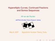
<strong>Paperfolding</strong>, <strong>Automata</strong>, <strong>and</strong> <strong>Rational</strong> <strong>Functions</strong><br />
<strong>Diagonals</strong> <strong>and</strong> Hadamard products of algebraic power series<br />
Alf van der Poorten<br />
ceNTRe for Number Theory Research, Sydney<br />
08 November, 2007 Laramie<br />
1
Abducted by an alien circus company, Professor Doyle<br />
is forced to write calculus equations in centre ring.<br />
3
<strong>Paperfolding</strong>, <strong>Automata</strong>, <strong>and</strong> <strong>Rational</strong> <strong>Functions</strong><br />
<strong>Diagonals</strong> <strong>and</strong> Hadamard products of algebraic power series<br />
Alf van der Poorten<br />
ceNTRe for Number Theory Research, Sydney<br />
08 November, 2007 Laramie<br />
4
<strong>Paperfolding</strong><br />
Take a rectangular sheet of paper <strong>and</strong> fold it in half, right half over left.<br />
Repeat the operation, <strong>and</strong> again, <strong>and</strong> again, <strong>and</strong> . . . . On unfolding the<br />
sheet of paper we see the creases as a sequence of valleys← 1 <strong>and</strong><br />
ridges← 0. Then, reading from left to right, after five folds we obtain<br />
We now recall that after one, two, three, four, five folds we saw<br />
1<br />
110<br />
1101100<br />
110110011100100<br />
1<br />
1101100111001001110110001100100<br />
so we obtain an infinite paperfolding sequence by adding a new middle<br />
fold 1 <strong>and</strong> noting that the second half of the sequence is the reverse<br />
mirror image of the first half. This justifies my adding . . . after those<br />
thirty-one creases.<br />
5
<strong>Paperfolding</strong><br />
Take a rectangular sheet of paper <strong>and</strong> fold it in half, right half over left.<br />
Repeat the operation, <strong>and</strong> again, <strong>and</strong> again, <strong>and</strong> . . . . On unfolding the<br />
sheet of paper we see the creases as a sequence of valleys← 1 <strong>and</strong><br />
ridges← 0. Then, reading from left to right, after five folds we obtain<br />
1 1<br />
We now recall that after one, two, three, four, five folds we saw<br />
1<br />
110<br />
1101100<br />
110110011100100<br />
1101100111001001110110001100100<br />
so we obtain an infinite paperfolding sequence by adding a new middle<br />
fold 1 <strong>and</strong> noting that the second half of the sequence is the reverse<br />
mirror image of the first half. This justifies my adding . . . after those<br />
thirty-one creases.<br />
5
<strong>Paperfolding</strong><br />
Take a rectangular sheet of paper <strong>and</strong> fold it in half, right half over left.<br />
Repeat the operation, <strong>and</strong> again, <strong>and</strong> again, <strong>and</strong> . . . . On unfolding the<br />
sheet of paper we see the creases as a sequence of valleys← 1 <strong>and</strong><br />
ridges← 0. Then, reading from left to right, after five folds we obtain<br />
1 1 0<br />
We now recall that after one, two, three, four, five folds we saw<br />
1<br />
110<br />
1101100<br />
110110011100100<br />
1101100111001001110110001100100<br />
so we obtain an infinite paperfolding sequence by adding a new middle<br />
fold 1 <strong>and</strong> noting that the second half of the sequence is the reverse<br />
mirror image of the first half. This justifies my adding . . . after those<br />
thirty-one creases.<br />
5
<strong>Paperfolding</strong><br />
Take a rectangular sheet of paper <strong>and</strong> fold it in half, right half over left.<br />
Repeat the operation, <strong>and</strong> again, <strong>and</strong> again, <strong>and</strong> . . . . On unfolding the<br />
sheet of paper we see the creases as a sequence of valleys← 1 <strong>and</strong><br />
ridges← 0. Then, reading from left to right, after five folds we obtain<br />
1 1 1 0<br />
We now recall that after one, two, three, four, five folds we saw<br />
1<br />
110<br />
1101100<br />
110110011100100<br />
1101100111001001110110001100100<br />
so we obtain an infinite paperfolding sequence by adding a new middle<br />
fold 1 <strong>and</strong> noting that the second half of the sequence is the reverse<br />
mirror image of the first half. This justifies my adding . . . after those<br />
thirty-one creases.<br />
5
<strong>Paperfolding</strong><br />
Take a rectangular sheet of paper <strong>and</strong> fold it in half, right half over left.<br />
Repeat the operation, <strong>and</strong> again, <strong>and</strong> again, <strong>and</strong> . . . . On unfolding the<br />
sheet of paper we see the creases as a sequence of valleys← 1 <strong>and</strong><br />
ridges← 0. Then, reading from left to right, after five folds we obtain<br />
1 1 0 1 0<br />
We now recall that after one, two, three, four, five folds we saw<br />
1<br />
110<br />
1101100<br />
110110011100100<br />
1101100111001001110110001100100<br />
so we obtain an infinite paperfolding sequence by adding a new middle<br />
fold 1 <strong>and</strong> noting that the second half of the sequence is the reverse<br />
mirror image of the first half. This justifies my adding . . . after those<br />
thirty-one creases.<br />
5
<strong>Paperfolding</strong><br />
Take a rectangular sheet of paper <strong>and</strong> fold it in half, right half over left.<br />
Repeat the operation, <strong>and</strong> again, <strong>and</strong> again, <strong>and</strong> . . . . On unfolding the<br />
sheet of paper we see the creases as a sequence of valleys← 1 <strong>and</strong><br />
ridges← 0. Then, reading from left to right, after five folds we obtain<br />
1 1 0 1 1 0<br />
We now recall that after one, two, three, four, five folds we saw<br />
1<br />
110<br />
1101100<br />
110110011100100<br />
1101100111001001110110001100100<br />
so we obtain an infinite paperfolding sequence by adding a new middle<br />
fold 1 <strong>and</strong> noting that the second half of the sequence is the reverse<br />
mirror image of the first half. This justifies my adding . . . after those<br />
thirty-one creases.<br />
5
<strong>Paperfolding</strong><br />
Take a rectangular sheet of paper <strong>and</strong> fold it in half, right half over left.<br />
Repeat the operation, <strong>and</strong> again, <strong>and</strong> again, <strong>and</strong> . . . . On unfolding the<br />
sheet of paper we see the creases as a sequence of valleys← 1 <strong>and</strong><br />
ridges← 0. Then, reading from left to right, after five folds we obtain<br />
1 1 0 1 1 0 0<br />
We now recall that after one, two, three, four, five folds we saw<br />
1<br />
110<br />
1101100<br />
110110011100100<br />
1101100111001001110110001100100<br />
so we obtain an infinite paperfolding sequence by adding a new middle<br />
fold 1 <strong>and</strong> noting that the second half of the sequence is the reverse<br />
mirror image of the first half. This justifies my adding . . . after those<br />
thirty-one creases.<br />
5
<strong>Paperfolding</strong><br />
Take a rectangular sheet of paper <strong>and</strong> fold it in half, right half over left.<br />
Repeat the operation, <strong>and</strong> again, <strong>and</strong> again, <strong>and</strong> . . . . On unfolding the<br />
sheet of paper we see the creases as a sequence of valleys← 1 <strong>and</strong><br />
ridges← 0. Then, reading from left to right, after five folds we obtain<br />
1 1 1 0 1 1 0 0<br />
We now recall that after one, two, three, four, five folds we saw<br />
1<br />
110<br />
1101100<br />
110110011100100<br />
1101100111001001110110001100100<br />
so we obtain an infinite paperfolding sequence by adding a new middle<br />
fold 1 <strong>and</strong> noting that the second half of the sequence is the reverse<br />
mirror image of the first half. This justifies my adding . . . after those<br />
thirty-one creases.<br />
5
<strong>Paperfolding</strong><br />
Take a rectangular sheet of paper <strong>and</strong> fold it in half, right half over left.<br />
Repeat the operation, <strong>and</strong> again, <strong>and</strong> again, <strong>and</strong> . . . . On unfolding the<br />
sheet of paper we see the creases as a sequence of valleys← 1 <strong>and</strong><br />
ridges← 0. Then, reading from left to right, after five folds we obtain<br />
1 1 0 1 0 1 1 0 0<br />
We now recall that after one, two, three, four, five folds we saw<br />
1<br />
110<br />
1101100<br />
110110011100100<br />
1101100111001001110110001100100<br />
so we obtain an infinite paperfolding sequence by adding a new middle<br />
fold 1 <strong>and</strong> noting that the second half of the sequence is the reverse<br />
mirror image of the first half. This justifies my adding . . . after those<br />
thirty-one creases.<br />
5
<strong>Paperfolding</strong><br />
Take a rectangular sheet of paper <strong>and</strong> fold it in half, right half over left.<br />
Repeat the operation, <strong>and</strong> again, <strong>and</strong> again, <strong>and</strong> . . . . On unfolding the<br />
sheet of paper we see the creases as a sequence of valleys← 1 <strong>and</strong><br />
ridges← 0. Then, reading from left to right, after five folds we obtain<br />
1 1 0 1 1 0 1 1 0 0<br />
We now recall that after one, two, three, four, five folds we saw<br />
1<br />
110<br />
1101100<br />
110110011100100<br />
1101100111001001110110001100100<br />
so we obtain an infinite paperfolding sequence by adding a new middle<br />
fold 1 <strong>and</strong> noting that the second half of the sequence is the reverse<br />
mirror image of the first half. This justifies my adding . . . after those<br />
thirty-one creases.<br />
5
<strong>Paperfolding</strong><br />
Take a rectangular sheet of paper <strong>and</strong> fold it in half, right half over left.<br />
Repeat the operation, <strong>and</strong> again, <strong>and</strong> again, <strong>and</strong> . . . . On unfolding the<br />
sheet of paper we see the creases as a sequence of valleys← 1 <strong>and</strong><br />
ridges← 0. Then, reading from left to right, after five folds we obtain<br />
1 1 0 1 1 0 0 1 1 0 0<br />
We now recall that after one, two, three, four, five folds we saw<br />
1<br />
110<br />
1101100<br />
110110011100100<br />
1101100111001001110110001100100<br />
so we obtain an infinite paperfolding sequence by adding a new middle<br />
fold 1 <strong>and</strong> noting that the second half of the sequence is the reverse<br />
mirror image of the first half. This justifies my adding . . . after those<br />
thirty-one creases.<br />
5
<strong>Paperfolding</strong><br />
Take a rectangular sheet of paper <strong>and</strong> fold it in half, right half over left.<br />
Repeat the operation, <strong>and</strong> again, <strong>and</strong> again, <strong>and</strong> . . . . On unfolding the<br />
sheet of paper we see the creases as a sequence of valleys← 1 <strong>and</strong><br />
ridges← 0. Then, reading from left to right, after five folds we obtain<br />
1 1 0 1 1 0 0 1 1 1 0 0<br />
We now recall that after one, two, three, four, five folds we saw<br />
1<br />
110<br />
1101100<br />
110110011100100<br />
1101100111001001110110001100100<br />
so we obtain an infinite paperfolding sequence by adding a new middle<br />
fold 1 <strong>and</strong> noting that the second half of the sequence is the reverse<br />
mirror image of the first half. This justifies my adding . . . after those<br />
thirty-one creases.<br />
5
<strong>Paperfolding</strong><br />
Take a rectangular sheet of paper <strong>and</strong> fold it in half, right half over left.<br />
Repeat the operation, <strong>and</strong> again, <strong>and</strong> again, <strong>and</strong> . . . . On unfolding the<br />
sheet of paper we see the creases as a sequence of valleys← 1 <strong>and</strong><br />
ridges← 0. Then, reading from left to right, after five folds we obtain<br />
1 1 0 1 1 0 0 1 1 1 0 0 0<br />
We now recall that after one, two, three, four, five folds we saw<br />
1<br />
110<br />
1101100<br />
110110011100100<br />
1101100111001001110110001100100<br />
so we obtain an infinite paperfolding sequence by adding a new middle<br />
fold 1 <strong>and</strong> noting that the second half of the sequence is the reverse<br />
mirror image of the first half. This justifies my adding . . . after those<br />
thirty-one creases.<br />
5
<strong>Paperfolding</strong><br />
Take a rectangular sheet of paper <strong>and</strong> fold it in half, right half over left.<br />
Repeat the operation, <strong>and</strong> again, <strong>and</strong> again, <strong>and</strong> . . . . On unfolding the<br />
sheet of paper we see the creases as a sequence of valleys← 1 <strong>and</strong><br />
ridges← 0. Then, reading from left to right, after five folds we obtain<br />
1 1 0 1 1 0 0 1 1 1 0 0 1 0<br />
We now recall that after one, two, three, four, five folds we saw<br />
1<br />
110<br />
1101100<br />
110110011100100<br />
1101100111001001110110001100100<br />
so we obtain an infinite paperfolding sequence by adding a new middle<br />
fold 1 <strong>and</strong> noting that the second half of the sequence is the reverse<br />
mirror image of the first half. This justifies my adding . . . after those<br />
thirty-one creases.<br />
5
<strong>Paperfolding</strong><br />
Take a rectangular sheet of paper <strong>and</strong> fold it in half, right half over left.<br />
Repeat the operation, <strong>and</strong> again, <strong>and</strong> again, <strong>and</strong> . . . . On unfolding the<br />
sheet of paper we see the creases as a sequence of valleys← 1 <strong>and</strong><br />
ridges← 0. Then, reading from left to right, after five folds we obtain<br />
1 1 0 1 1 0 0 1 1 1 0 0 1 0 0<br />
We now recall that after one, two, three, four, five folds we saw<br />
1<br />
110<br />
1101100<br />
110110011100100<br />
1101100111001001110110001100100<br />
so we obtain an infinite paperfolding sequence by adding a new middle<br />
fold 1 <strong>and</strong> noting that the second half of the sequence is the reverse<br />
mirror image of the first half. This justifies my adding . . . after those<br />
thirty-one creases.<br />
5
<strong>Paperfolding</strong><br />
Take a rectangular sheet of paper <strong>and</strong> fold it in half, right half over left.<br />
Repeat the operation, <strong>and</strong> again, <strong>and</strong> again, <strong>and</strong> . . . . On unfolding the<br />
sheet of paper we see the creases as a sequence of valleys← 1 <strong>and</strong><br />
ridges← 0. Then, reading from left to right, after five folds we obtain<br />
1101100111001001110110001100100<br />
We now recall that after one, two, three, four, five folds we saw<br />
1<br />
110<br />
1101100<br />
110110011100100<br />
1101100111001001110110001100100<br />
so we obtain an infinite paperfolding sequence by adding a new middle<br />
fold 1 <strong>and</strong> noting that the second half of the sequence is the reverse<br />
mirror image of the first half. This justifies my adding . . . after those<br />
thirty-one creases.<br />
5
<strong>Paperfolding</strong><br />
Take a rectangular sheet of paper <strong>and</strong> fold it in half, right half over left.<br />
Repeat the operation, <strong>and</strong> again, <strong>and</strong> again, <strong>and</strong> . . . . On unfolding the<br />
sheet of paper we see the creases as a sequence of valleys← 1 <strong>and</strong><br />
ridges← 0. Then, reading from left to right, after five folds we obtain<br />
1101100111001001110110001100100 . . .<br />
We now recall that after one, two, three, four, five folds we saw<br />
1<br />
110<br />
1101100<br />
110110011100100<br />
1101100111001001110110001100100 . . .<br />
so we obtain an infinite paperfolding sequence by adding a new middle<br />
fold 1 <strong>and</strong> noting that the second half of the sequence is the reverse<br />
mirror image of the first half. This justifies my adding . . . after those<br />
thirty-one creases.<br />
5
A Mahler Functional Equation<br />
Aside. Is the number 0.11011001110010011101100011001001 . . .<br />
transcendental?<br />
Now consider subtracting the spaced out sequence from the<br />
paperfolding sequence:<br />
If we denote the paperfolding sequence by f1, f2, f3, . . . then we have<br />
verified experimentally that the formal power series F (X) = P∞ h=1<br />
satisfies the functional equation F(X) − F(X 2 ) = X/(1 − X 4 ) .<br />
fhX h<br />
Once noticed, we see that this is obvious. Inserting an extra positive<br />
fold is to replace F (X) by F(X 2 ) <strong>and</strong> to add X/(1 − X 4 ). However, the<br />
infinite paperfolding sequence is invariant under the addition of a<br />
positive fold.<br />
6
A Mahler Functional Equation<br />
Aside. Is the number 0.11011001110010011101100011001001 . . .<br />
transcendental?<br />
Now consider subtracting the spaced out sequence from the<br />
paperfolding sequence:<br />
1 1 0 1 1 0 0 1 1 1 0 0 1 0 0 1 1 1 0 1 1 0 0 0<br />
If we denote the paperfolding sequence by f1, f2, f3, . . . then we have<br />
verified experimentally that the formal power series F(X) = P∞ h=1<br />
satisfies the functional equation F(X) − F(X 2 ) = X/(1 − X 4 ) .<br />
fhX h<br />
Once noticed, we see that this is obvious. Inserting an extra positive<br />
fold is to replace F (X) by F(X 2 ) <strong>and</strong> to add X/(1 − X 4 ). However, the<br />
infinite paperfolding sequence is invariant under the addition of a<br />
positive fold.<br />
6
A Mahler Functional Equation<br />
Aside. Is the number 0.11011001110010011101100011001001 . . .<br />
transcendental?<br />
Now consider subtracting the spaced out sequence from the<br />
paperfolding sequence:<br />
1101100111001001110110001100100111011001110010001 . . .<br />
we get<br />
1 1 0 1 1 0 0 1 1 1 0 0 1 0 0 1 1 1 0 1 1 0 0 0<br />
1000100010001000100010001000100010001000100010001 . . .<br />
If we denote the paperfolding sequence by f1, f2, f3, . . . then we have<br />
verified experimentally that the formal power series F(X) = P∞ h=1<br />
satisfies the functional equation F(X) − F(X 2 ) = X/(1 − X 4 ) .<br />
fhX h<br />
Once noticed, we see that this is obvious. Inserting an extra positive<br />
fold is to replace F(X) by F(X 2 ) <strong>and</strong> to add X/(1 − X 4 ). However, the<br />
infinite paperfolding sequence is invariant under the addition of a<br />
positive fold.<br />
6
Next, if we pair the sequence<br />
Regular Binary Substitution<br />
11.01.10.01.11.00.10.01.11.01.10.00.11.00.10.01.<br />
11.01.10.01.11.00.10.00.11.01.10.00.11.00.10.01. . . .<br />
<strong>and</strong> interpret the pairs as numbers in base 2, we obtain<br />
3.1.2.1.3.0.2.1.3.1.2.0.3.0.2.1.3.1.2.1.3.0.2.0.3.1.2.0.3.0.2.1. . . .<br />
But this is precisely the original sequence warmed up by adding 2 to<br />
every second entry:<br />
31.21.30.21.31.20.30.21.31.21.30.20.31.20.30.21.<br />
31.21.30.21.31.20.30.20.31.21.30.20.30.21. . . .<br />
Thus, experimentally at any rate, the new sequence, which I again call<br />
(fh), is invariant under the uniform binary substitution<br />
θ : 0 ↦→ 20, 1 ↦→ 21, 2 ↦→ 30, 3 ↦→ 31.<br />
7
The uniform, or regular, 2-substitution<br />
θ : 0 ↦→ 20, 1 ↦→ 21, 2 ↦→ 30, 3 ↦→ 31.<br />
provides a transition map τ defined by the transition table:<br />
τ 0 1<br />
s3 s3 s1<br />
s2 s3 s0<br />
s1 s2 s1<br />
s0 s2 s0<br />
The transition table shows how each state si responds to the input of a<br />
binary digit <strong>and</strong> makes plain that we are dealing with a finite state<br />
automaton; specifically a four-state automaton; s3 is its initial state.<br />
The automaton provides a map h ↦→ fh+1 . Consider an input tape<br />
containing the digits of h written in base 2. The automaton reads the<br />
digits of h successively, disregarding initial zeros because they leave<br />
the automaton in state s3 . Finally an output map replaces s3 or s1 by<br />
1, <strong>and</strong> s2 or s0 by 0, yielding fh+1 .<br />
8
Characteristic <strong>Functions</strong><br />
I found the formation rule by viewing the symbols in pairs as binary<br />
integers <strong>and</strong> noticing that the resulting sequence is self reproducing<br />
under the substitution θ. However, let Fi(X) = P<br />
fh=i X h be the<br />
characteristic function of each of the symbols i = 0, 1, 2, <strong>and</strong> 3. It’s<br />
not difficult to see from the defining substitution θ, that in fact<br />
F0(X) = F0(X 2 ) + F2(X 2 ), XF2(X) = F0(X 2 ) + F1(X 2 ),<br />
F1(X) = F1(X 2 ) + F3(X 2 ), XF3(X) = F2(X 2 ) + F3(X 2 ).<br />
Moreover, by definition, F0(X) + F1(X) + F2(X) + F3(X) = X/(1 − X),<br />
<strong>and</strong> of course F1(X) + F3(X) = F(X). In this way a trick to ‘guess’ the<br />
Mahler functional equation<br />
F(X) = F(X 2 ) + X/(1 − X 4 )<br />
is replaced by a dull <strong>and</strong> uninstructive systematic proof.<br />
Mind you, a function F(X 2 ), more generally F(X p ), seems unnatural.<br />
One should wonder how such a function might arise naturally.<br />
9
An Algebraic Equation in Characteristic p<br />
For a prime p, <strong>and</strong> for G any formal power series with integer<br />
coefficients,<br />
G(X p ) ≡ (G(X)) p mod p; equivalently G(X p ) = (G(X)) p<br />
in the ring Fp[[X]] of formal power series over the finite field Fp of p<br />
elements. This is plain because the Frobenius map x ↦→ x p is an<br />
additive automorphism (that is: by Fermat’s Little Theorem <strong>and</strong><br />
because all the multinomial coefficients other than those on the<br />
diagonal vanish modulo p). Hence the Mahler functional equation<br />
(1 − X 4 )F(X) 2 − (1 − X 4 )F(X) + X = 0<br />
for F = F1 + F3 becomes the equation<br />
(1 + X) 4 F 2 + (1 + X) 4 F + X = 0 ,<br />
showing that F is an algebraic element over F2[[X]].<br />
In general, a linear relation on 1, F(X), F(X p ), . . . , over Z[X]<br />
reduces to an algebraic equation over over Fp[X] linearly relating<br />
1, F , F p , . . . .<br />
10
These remarks show that the paperfolding sequence (fh) is<br />
(i) (an image of) a sequence invariant under the substitution θ <strong>and</strong> is<br />
(ii) therefore given by limh→∞ θ h (3), where θ(3) = 31,<br />
θ 2 (3) = θ(31) = θ(3)θ(1) = 3121, . . . .<br />
(iii) It follows that the sequence is 2-automatic, that is there are only<br />
finitely many distinct subsequences {f 2 k h+r : k ≥ 0, 0 ≤ r < 2 k };<br />
in the present case (fh) itself, <strong>and</strong> the purely periodic sequences<br />
with period 0, 1, or 10.<br />
(iv) Equivalently the corresponding transition map defines a finite state<br />
automaton which maps h ↦→ fh+1 , or, if one prefers,<br />
(v) the substitution defines a system of Mahler functional equations<br />
satisfied by the characteristic function of each state <strong>and</strong> therefore<br />
such an equation satisfied by the paperfolding function.<br />
(vi) Reduction mod 2 of that equation yields an algebraic equation for<br />
the paperfolding function over F2(X).<br />
11
The Thue-Morse Sequence<br />
0 1 10 11 100 101 110 111 1000 1001 1010 1011 1100 1101 . . .<br />
0 1 1 0 1 0 0 1 1 0 0 1 0 1 . . .<br />
The Thue-Morse sequence<br />
(sh)h≥0 := 0110100110 0101101001 0110011010 0110 . . . ,<br />
lays compelling claim to being the simplest nontrivial (non-periodic)<br />
sequence. It is generated by the rule that sh ≡: s2(h) (mod 2).<br />
Here, sp(h) denotes the sum of the digits of h written in base p. The<br />
function sp(h) crops up in real life in the following way: It is a cute<br />
exercise to confirm that the precise power, ordp h!, to which a prime p<br />
divides h! is ordp h! = ` h − sp(h) ´ /(p − 1) .<br />
More, suppose a + b = c in nonnegative integers a, b, <strong>and</strong> c . Then<br />
s2(a) + s2(b) − s2(c) is both the number<br />
´<br />
of carries required when<br />
adding a to b in binary; <strong>and</strong> is ord2 .<br />
` a+b<br />
a<br />
12
Euler’s Identity <strong>and</strong> a Functional Equation<br />
Fairly obviously, the sequence (sh) is invariant under the uniform<br />
binary substitution θ : 0 ↦→ 01 <strong>and</strong> 1 ↦→ 10. Now recall Euler’s identity<br />
∞Y “<br />
1 + X 2n”<br />
=<br />
n=0<br />
∞X<br />
h=0<br />
X h = 1<br />
1 − X ,<br />
noting it is just a pleasant way of recalling that the nonegative integers<br />
each have a unique representation in base 2. It will then also be fairly<br />
obvious that<br />
T (X) :=<br />
∞Y “<br />
1 − X 2n”<br />
=<br />
n=0<br />
∞X<br />
(−1) sh h<br />
X ;<br />
<strong>and</strong> that plainly T (X) = P ∞<br />
h=0 (−1)s hX h satisfies the Mahler functional<br />
equation<br />
(1 − X)T (X 2 ) = T (X) .<br />
h=0<br />
13
An Algebraic Equation<br />
The function S(X) = P ∞<br />
h=0 shX h therefore satisfies<br />
(1 − X 2 )(1 − X)S(X 2 ) − (1 − X 2 )S(X) + X = 0 .<br />
Exercise. Show that for an arbitrary sequence (ih), with ih ∈ {0, 1},<br />
one has P (−1) i hX h = (1 − X) −1 − 2 P ihX h , <strong>and</strong> hence confirm the<br />
“therefore” above.<br />
Hence, reducing modulo 2, we see that over the finite field F2 we have<br />
(1 + X) 3 S 2 + (1 + X) 2 S + X = 0 ,<br />
showing that S is quadratic irrational over the field F2(X).<br />
14
A Counter-example in Analysis<br />
I claim that, whatever the choice of signs ±,<br />
max<br />
0≤θ≤1 |<br />
n−1<br />
h=0<br />
X<br />
±e 2πihθ | ≥ √ n.<br />
Indeed, by well known orthogonality relations,<br />
Z 1 ˛<br />
˛Xn−1<br />
˛ ±e 2πihθ<br />
˛ 2<br />
dθ = n.<br />
0<br />
h=0<br />
But what is min± max0≤θ≤1 | Pn−1 h=0 ±e2πihθ |?<br />
After suitable statistical incantations, almost surely<br />
min max<br />
± 0≤θ≤1 |<br />
n−1<br />
h=0<br />
X<br />
±e 2πihθ | = O( √ n log log n).<br />
Perhaps the correct question is: What choices (i0, . . . , in−1) minimise<br />
max<br />
0≤θ≤1 |<br />
n−1<br />
h=0<br />
X<br />
(−1) ih 2πihθ<br />
e | ?<br />
15
The Shapiro Sequence<br />
Consider, the Shapiro sequence (rh), which counts mod 2 the number<br />
of occurrences of the pair 11 of digits in the binary expansion of h.<br />
0001001000 0111010001 0010111000 1000010010 0001110111 . . .<br />
0 1 0 2 0 1 3 1 0 1 0 2 3 2 0 2 0 1 0 2 0 1 3 1 3 . . .<br />
0001001000 0111010001 0010111000 1000010010 0001110111 . . .<br />
So, the Shapiro sequence is<br />
generated by the automaton defined by the transition table given by θ<br />
<strong>and</strong> with output map s0 <strong>and</strong> s1 ← 0, <strong>and</strong> s2 <strong>and</strong> s3 ← 1. Remarkably<br />
n−1<br />
max<br />
0≤θ≤1 |<br />
X<br />
(−1) r √ √<br />
h ihθ<br />
e | ≤ (2 + 2) n .<br />
h=0<br />
16
The Shapiro Sequence<br />
Consider, the Shapiro sequence (rh), which counts mod 2 the number<br />
of occurrences of the pair 11 of digits in the binary expansion of h.<br />
0001001000 0111010001 0010111000 1000010010 0001110111 . . .<br />
0 1 0 2 0 1 3 1 0 1 0 2 3 2 0 2 0 1 0 2 0 1 3 1 3 . . .<br />
0001001000 0111010001 0010111000 1000010010 0001110111 . . .<br />
Here the blue sequence is the result of an ingenious pairing<br />
So, the Shapiro sequence is<br />
generated by the automaton defined by the transition table given by θ<br />
<strong>and</strong> with output map s0 <strong>and</strong> s1 ← 0, <strong>and</strong> s2 <strong>and</strong> s3 ← 1. Remarkably<br />
n−1<br />
max<br />
0≤θ≤1 |<br />
X<br />
(−1) r √ √<br />
h ihθ<br />
e | ≤ (2 + 2) n .<br />
h=0<br />
16
The Shapiro Sequence<br />
Consider, the Shapiro sequence (rh), which counts mod 2 the number<br />
of occurrences of the pair 11 of digits in the binary expansion of h.<br />
0001001000 0111010001 0010111000 1000010010 0001110111 . . .<br />
0 1 0 2 0 1 3 1 0 1 0 2 3 2 0 2 0 1 0 2 0 1 3 1 3 . . .<br />
0102013101 0232020102 0131323101 3101020131 0102320232 . . .<br />
0001001000 0111010001 0010111000 1000010010 0001110111 . . .<br />
Here the blue sequence is the result of an ingenious pairing; the brown<br />
sequence then recognises that (rh) is given by the regular binary<br />
substitution θ : 0 ↦→ 01, 1 ↦→ 02, 2 ↦→ 31, 3 ↦→ 32.<br />
The intermediate symbols {0, 1, 2, 3} represent the four states<br />
{s0, s1, s2, s3} of a binary automaton. So, the Shapiro sequence is<br />
generated by the automaton defined by the transition table given by θ<br />
<strong>and</strong> with output map s0 <strong>and</strong> s1 ← 0, <strong>and</strong> s2 <strong>and</strong> s3 ← 1. Remarkably<br />
n−1<br />
max<br />
0≤θ≤1 |<br />
X<br />
(−1) r √ √<br />
h ihθ<br />
e | ≤ (2 + 2) n .<br />
h=0<br />
16
A Remark on the Shapiro Function<br />
Separating the even <strong>and</strong> odd placed elements of (rh), we see that<br />
This same/different rule makes it surprisingly easy to write the<br />
sequence from scratch. The second row is (r2h) . Remarkably, it<br />
coincides with the original sequence, illustrating that rh = r2h . The<br />
third row is (r2h+1) . With careful attention, we see that r4h = r4h+1 but<br />
r4h+2 = r4h+3 . Setting P(X) = P (−1) r hX h , these observations<br />
amount to the functional equation<br />
P(X) = P(X 2 ) + XP(−X 2 ) .<br />
By an earlier exercise, <strong>and</strong> some pain, the function R(X) = P rhX h<br />
satisfies the functional equation<br />
2X(1 − X 4 )R(X 4 ) + (1 − X 4 )(1 − X)R(X 2 ) − (1 − X 4 )R(X) + X 3 = 0 .<br />
Does the algebraic equation over F2(X) already define the function?<br />
17
A Remark on the Shapiro Function<br />
Separating the even <strong>and</strong> odd placed elements of (rh), we see that<br />
0 0 0 1 0 0 1 0 0 0 0 1 1 1 0 1 0 0 0 1 0 0 1 0 1 . . .<br />
0 1 0 0 0 1 1 1 0 1 0 0 1 0 0 0 0 1 0 0 0 1 1 1 1 . .<br />
This same/different rule makes it surprisingly easy to write the<br />
sequence from scratch. The second row is (r2h) . Remarkably, it<br />
coincides with the original sequence, illustrating that rh = r2h . The<br />
third row is (r2h+1) . With careful attention, we see that r4h = r4h+1 but<br />
r4h+2 = r4h+3 . Setting P(X) = P (−1) r hX h , these observations<br />
amount to the functional equation<br />
P(X) = P(X 2 ) + XP(−X 2 ) .<br />
By an earlier exercise, <strong>and</strong> some pain, the function R(X) = P rhX h<br />
satisfies the functional equation<br />
2X(1 − X 4 )R(X 4 ) + (1 − X 4 )(1 − X)R(X 2 ) − (1 − X 4 )R(X) + X 3 = 0 .<br />
Does the algebraic equation over F2(X) already define the function?<br />
17
A Remark on the Shapiro Function<br />
Separating the even <strong>and</strong> odd placed elements of (rh), we see that<br />
0001001000 0111010001 0010111000 1000010010 0001110111 . . .<br />
0 0 0 1 0 0 1 0 0 0 0 1 1 1 0 1 0 0 0 1 0 0 1 0 1 . . .<br />
0 1 0 0 0 1 1 1 0 1 0 0 1 0 0 0 0 1 0 0 0 1 1 1 1 . .<br />
This same/different rule makes it surprisingly easy to write the<br />
sequence from scratch. The second row is (r2h) . Remarkably, it<br />
coincides with the original sequence, illustrating that rh = r2h . The<br />
third row is (r2h+1) . With careful attention, we see that r4h = r4h+1 but<br />
r4h+2 = r4h+3 . Setting P(X) = P (−1) r hX h , these observations<br />
amount to the functional equation<br />
P(X) = P(X 2 ) + XP(−X 2 ) .<br />
By an earlier exercise, <strong>and</strong> some pain, the function R(X) = P rhX h<br />
satisfies the functional equation<br />
2X(1 − X 4 )R(X 4 ) + (1 − X 4 )(1 − X)R(X 2 ) − (1 − X 4 )R(X) + X 3 = 0 .<br />
Does the algebraic equation over F2(X) already define the function?<br />
17
Transcendence of Automatic Numbers<br />
In the eighties, John Loxton <strong>and</strong> I proved transcendence results on<br />
values of Mahler functions giving strong support for the belief that the<br />
decimal expansion (more generally the base b expansion) of an<br />
irrational algebraic number cannot be generated by a finite automaton.<br />
For instance, it is a theorem that in any base b the paperfolding<br />
number 0.110110011100100111011000110 . . . is transcendental.<br />
In consequence the matter of the transcendence of irrational automatic<br />
numbers became known in the trade as the conjecture of Loxton <strong>and</strong><br />
van der Poorten.<br />
But our results did not cover all cases <strong>and</strong> had significant exceptions<br />
skew to the motivating problem <strong>and</strong> plainly caused by technical<br />
difficulties inherent in our methods.<br />
Fortunately, a much more appropriate argument has now been found<br />
by Boris Adamczewski <strong>and</strong> Yann Bugeaud (Strassbourg).<br />
19
Complexity of a Sequence<br />
Given an infinite string, denote by p(n) the number of its distinct<br />
subwords of length n. Almost all numbers (in base b) have p(n) = b n ;<br />
but sequences generated by a finite automaton have only a miserable<br />
complexity p(n) = O(n).<br />
Not all that long ago, BORIS ADAMCZEWSKI, YANN BUGEAUD, AND<br />
FLORIAN LUCA, ‘Sur la complexité des nombres algébriques’, C. R.<br />
Acad. Sci. Paris, Ser. I 336 (2004), applied Schlickewei’s p-adic<br />
generalisation of Wolfgang Schmidt’s subspace theorem (which is itself<br />
a multidimensional generalisation of Roth’s theorem) to proving that for<br />
the base b expansion of an irrational algebraic number<br />
lim inf p(n)/n = +∞.<br />
n→∞<br />
A more detailed paper usefully generalising the earlier announcement:<br />
‘On the complexity of algebraic numbers’, by BORIS ADAMCZEWSKI<br />
AND YANN BUGEAUD, has now appeared in Annals of Math.<br />
20
Algebraicity <strong>and</strong> Automaticity<br />
The phenomena we have just now noticed<br />
1 automaticity<br />
2 algebraicity in characteristic p<br />
3 Mahler functional equation<br />
4 regular p-substitutions<br />
are equivalent.<br />
It is a theorem of Giles Christol, Teturo Kamae, Michel Mendès France,<br />
<strong>and</strong> Gérard Rauzy that the Taylor coefficients of a power series defined<br />
over a finite field of characteristic p provide a p-automatic sequence if<br />
<strong>and</strong> only if the power series represents an algebraic function.<br />
Remarks of Loxton <strong>and</strong> mine add the identification with Mahler<br />
functions in characteristic zero.<br />
22
Comments on the Proof<br />
The best proof (in my opinion) is due to Jan Denef <strong>and</strong> Leonard<br />
Lipshitz <strong>and</strong> relies on studying formal power series in many variables<br />
with coefficients from a finite field, say Fp .<br />
Given polynomials P <strong>and</strong> Q in just two variable x <strong>and</strong> y , <strong>and</strong> with<br />
Q(0, 0) = 0, suppose one were forced to look at the series expansion<br />
P(x, y)/Q(x, y) =<br />
∞X<br />
n=0 m=0<br />
∞X<br />
anmx n y m .<br />
It is arguably natural to recoil in fright <strong>and</strong> to insist on following a<br />
suggestion of Furstenberg to study just its diagonal P ∞<br />
n=0 annx n .<br />
It turns out to be not hard to prove that the complete diagonal of a<br />
rational function in two variables always is an algebraic function.<br />
23
But for expansions over the complex numbers C, the complete<br />
diagonal of a power series of a rational function in more than two<br />
variables is in general not algebraic.<br />
It is a beautiful fact that it is, however, a G-function, a power series inter<br />
alia satisfying a linear differential equation with polynomial coefficients.<br />
However, for expansions over a finite field, say Fp , diagonals of a<br />
rational function always are algebraic. Conversely, every algebraic<br />
power series in n variables is a diagonal of a rational function in at<br />
most 2n variables.<br />
More, the Taylor coefficients of such an algebraic power series are<br />
readily shown to satisfy congruence conditions which amount to the<br />
sequence plainly being generated by a p-automaton. I might remark<br />
that those congruences also were noticed independently by Pierre<br />
Deligne, some years after the CKMR proof. Indeed, Denef <strong>and</strong> Lipshitz<br />
tell me they developed their arguments after giving up on trying to<br />
underst<strong>and</strong> Deligne’s proof.<br />
24
Power Series in Several Variables<br />
R[[x]] is the ring of formal power series in x = (x1, . . . , xn).<br />
I write a series f (x) ∈ R[[x]] as f (x) = P ai 1···in x i 1<br />
where ν = (ν1, . . . , νn) is a multi-index <strong>and</strong> x ν = x ν 1<br />
1<br />
1<br />
· · · x in<br />
n = P aνx ν<br />
· · · x νn<br />
n .<br />
Below, R is usually the finite field Fp of p elements or the ring of<br />
p-adic integers Zp .<br />
One says that f (x) ∈ R[[x]] is algebraic if it is algebraic over the<br />
quotient field of the polynomial ring R[x]. I say that f (x) ∈ Zp[[x]] is<br />
algebraic mod p s if there is an algebraic g(x) ∈ Zp[[x]] with f ≡ g<br />
mod p s .<br />
Given f (x, y) = P aijx i y j it is natural to refer to the series<br />
Ixyf = P aiix i as its diagonal.<br />
Given f (x) = P ai 1···in x i 1<br />
1<br />
I12f = P ai 1i 1i 3···in x i 1<br />
1 x i3 3<br />
· · · x in<br />
n we define its diagonal I12f by<br />
· · · x in<br />
n ; generally, for k = l , the other Ikl are<br />
defined correspondingly. By a diagonal we mean any composition of<br />
the Ikl s. The complete diagonal is If = P aii···ix i 1 .<br />
26
<strong>Diagonals</strong> <strong>and</strong> Hadamard Products<br />
The Hadamard product of series f (x) = P aνx ν <strong>and</strong> g(x) = P bνx ν<br />
is the student product<br />
f ∗ g(x) = X aνbνx ν .<br />
<strong>Diagonals</strong> <strong>and</strong> Hadamard products are connected by:<br />
f ∗ g(x) = I1,n+1 . . . In,2nf (x1, . . . , xn)g(xn+1, . . . , x2n) ;<br />
I12f = f ∗ ` nY 1 1 ´<br />
.<br />
1 − x1x2 1 − xj<br />
j=3<br />
If a ring of power series is closed under one of the two operations of<br />
taking diagonals or Hadamard products then it is closed under the<br />
other operation. Over C, the diagonal is also given by the integral<br />
I12f (t, x3, . . . , xn) = 1<br />
I<br />
f (x1, . . . , xn)<br />
2πi<br />
dx1 ∧ dx2<br />
dt<br />
x 1x 2=t<br />
= 1<br />
2πi<br />
I<br />
|y|=ɛ<br />
f (t/y, y, x3, . . . , xn)dy/y .<br />
27
A Theorem of Furstenberg<br />
It follows that the diagonal of a rational function f (x, y) of two variables<br />
is an algebraic function. Indeed,<br />
(If )(t) = 1<br />
2πi<br />
I<br />
|y|=ɛ<br />
f (t/y, y) dy<br />
y<br />
1<br />
=<br />
2πi<br />
I<br />
|y|=ɛ<br />
P(t, y)<br />
dy .<br />
Q(t, y)<br />
Writing Q(t, y) = Q` y − yi(t) ´ , where the yi(t) are algebraic, <strong>and</strong><br />
evaluating the integral by residues verifies the claim.<br />
In fact, every algebraic power series of one variable is the diagonal of a<br />
rational power series of two variables <strong>and</strong>, indeed, every algebraic<br />
power series in n variables is the diagonal of a rational power series in<br />
2n variables.<br />
Below I sketch a proof showing that every diagonal of a rational<br />
function defined over a finite field is algebraic. However, in<br />
characteristic zero diagonals of rational functions in more than two<br />
variables do not generally yield algebraic functions.<br />
28
As said, in characteristic zero, neither diagonals, nor Hadamard<br />
products, preserve algebraicity. For the latter, the st<strong>and</strong>ard example is<br />
(1 − 4X) −1/2 = X “<br />
2h<br />
”<br />
X<br />
h<br />
h ; but X “<br />
2h<br />
h<br />
is not algebraic. The first remark is just the useful identity<br />
“<br />
2h<br />
”<br />
h<br />
= (−4) h“ −1/2<br />
”<br />
h<br />
”2<br />
X h<br />
Facts such as this are of interest to logicians.Then, introductory<br />
calculus shows the latter series is given by the integral<br />
Z π/2 2<br />
π 0<br />
dt<br />
q<br />
(1 − 16X sin 2 t)<br />
This is a complete elliptic integral well known not to represent an<br />
algebraic function.<br />
.<br />
29
A Beautiful Transcendence Argument<br />
For general odd k the question of the transcendence of the Hadamard<br />
powers<br />
Fk(X) = X “ ”k<br />
2h<br />
X<br />
h<br />
h<br />
had long been open, until delightfully settled by a remark of Sharif <strong>and</strong><br />
Woodcock.<br />
On the one h<strong>and</strong>, one views Fk as defined over Fp , so that certainly<br />
F p<br />
k = Fk <strong>and</strong> plainly Fk has degree dividing p − 1. However, it is easy<br />
to see that given any lower bound r there are infinitely many odd<br />
primes p so that p − 1 is divisible only by 1, 2, <strong>and</strong> primes greater<br />
than r .<br />
Exercise. One also confirms fairly readily that Fk is neither rational nor<br />
of degree 2 over Fp for infinitely many p.<br />
On the other h<strong>and</strong>, if Fk defined over Q were algebraic, say of degree<br />
r , then obviously its reduction mod p also is algebraic of degree at<br />
most r .<br />
30
Breaking Up in Characteristic p<br />
The following breaking up procedure is fundamental below:<br />
{x α = x α 1<br />
1<br />
· · · x αn<br />
n : α ∈ S} is a basis for Fp[[x]] over ` Fp[[x]] ´ p .<br />
Hence if y(x) ∈ Fp[[x]] <strong>and</strong> S = {0, 1, . . . , p − 1} n then, for α ∈ S ,<br />
there are unique yα(x) ∈ Fp[[x]] such that y(x) = P<br />
α∈S x α y p α(x) .<br />
If y(x) ∈ Fp[[x]] is algebraic then y satisfies an equation of the shape<br />
sX<br />
i=r<br />
fi(x)y pi<br />
= 0 ,<br />
with r , s ∈ N , the fi ∈ Fp[x] <strong>and</strong> fr = 0 . In fact, we may take r = 0 ,<br />
for if r > 0 then writing fi = P<br />
α x αf p<br />
we get that<br />
iα<br />
Hence Ps−1 pi<br />
i=r−1<br />
fi+1,α(x)y<br />
X<br />
x α` s X<br />
fiα(x)y pi−1´ p<br />
= 0 .<br />
α<br />
i=r<br />
= 0 <strong>and</strong> some frα = 0 .<br />
31
Algebraic power series in characteristic p<br />
Thus if y ∈ Fp[[x]] is algebraic, y satisfies an equation of the shape<br />
sX<br />
f (x)y = fi(x)y pi<br />
= L ` y p , . . . , y ps´ ,<br />
i=1<br />
where L is linear with coefficients polynomials in x . After multiplying<br />
by f p−1 , breaking up y <strong>and</strong> the coefficients of L, <strong>and</strong> then taking p-th<br />
roots, we get equations<br />
` p p<br />
f (x)yα1 = Lα1 y, y , . . . , y s−1´<br />
.<br />
Now multiplying by f p−1 <strong>and</strong> substituting for f (x)y on the right yields<br />
f p yα1 = Lα1 (f p−2 L(y p , . . . , y ps<br />
), f p−1 y p , . . . , f p−1 y ps−1<br />
) ,<br />
which again is linear in y p ,. . . , y ps . This brings us back, more or less,<br />
to the start <strong>and</strong> shows that iterating the process described leads to<br />
equations of the shape<br />
` p p<br />
f (x)yα1...αe = Lα1...αe y, y , . . . , y s−1´<br />
.<br />
If, during this procedure, we keep track of the (multi-) degree in x of<br />
Lα 1...αe we see that degree remains bounded.<br />
32
Hence, since Fp is finite, there are only a finite number of distinct<br />
yα 1...αe <strong>and</strong> we have a result of Christol, Kamae, Mendès France, <strong>and</strong><br />
Rauzy, here proved by the elegant independent methods of Jan Denef<br />
<strong>and</strong> Leonard Lipshitz.<br />
Theorem. If y = P aνx ν is algebraic then<br />
(F) there is an e such that for every (α1, . . . , αe) ∈ Se there is an<br />
e ′ < e <strong>and</strong> a (β1, . . . , βe ′) ∈ Se′<br />
such that<br />
yα 1...αe = yβ 1...β e ′ ;<br />
(A) equivalently, there is an e such that for all j = (j1, . . . , jn) with the<br />
ji < pe there is an e ′ < e <strong>and</strong> a j ′ = (j ′ 1 , . . . , j′ n) with the j ′<br />
i < pe′<br />
such that<br />
ap e ν+j = a p e ′ ν+j ′ for all ν .<br />
Conversely, if y satisfies (F) then taking yβ 1...β e ′ <strong>and</strong> breaking it up<br />
e − e ′ times, we see that the yα 1...αe satisfy a system of the form<br />
yα 1...αe = X x γ y pe−e′<br />
β 1...βe .<br />
By an easy lemma it follows that the yα 1...αe , <strong>and</strong> hence y , must be<br />
algebraic.<br />
33
Suppose the series P aνx ν is generated by a finite automaton M .<br />
Choose e so large that every state that M enters in the course of any<br />
computation is entered in a computation of length less than e . Then<br />
the aν satisfy version (A) of the Theorem.<br />
Conversely, if the aν satisfy (A) one can construct a finite automaton<br />
M that generates P aνx ν .<br />
M will be equipped with a table detailing the identifications (A) <strong>and</strong> an<br />
output list of the values of the aj for j = (j1, . . . , jn) with the ji < p e .<br />
The automaton M computes as follows: It reads e digits from each<br />
tape. Then it uses the table (A) to replace those e digits by e ′ digits. It<br />
reads a further e − e ′ digits <strong>and</strong> iterates. At each stage it outputs the<br />
appropriate value from its output list.<br />
34
So we have:<br />
Theorem. P aνx ν ∈ Fp[[x]] is algebraic if <strong>and</strong> only if it is generated by<br />
a finite automaton.<br />
Corollary. And so: Let f , g ∈ Fp[[x]] be algebraic. Then<br />
(i) Every diagonal of f is algebraic, as is every off-diagonal.<br />
(ii) The Hadamard product f ∗ g is algebraic.<br />
(iii) Irrelevance of symbols: Each characteristic series f (i) = P<br />
is algebraic.<br />
aν=i x ν<br />
We have already noted that the situation in characteristic zero is very<br />
different.<br />
Indeed, in characteristic zero there is a theorem of Polyá –Carleson by<br />
which a power series with integer coefficients <strong>and</strong> radius of<br />
convergence 1 is either rational or has the unit circle as a natural<br />
boundary. Thus the Mahler functions mentioned here all are<br />
transcendental functions.<br />
35
The Lifting Theorem<br />
Looking carefully, one sees that every algebraic power series in Fp[[x]]<br />
is the reduction of an algebraic power series in Zp[[x]] .<br />
Conversely there is an surprising lifting theorem (Loxton <strong>and</strong> vdP)<br />
whereby every algebraic power series in Fp[[x]] is found to lift to a<br />
series in Z[[x]] which is a solution of a system of functional equations.<br />
Note the example of the Shapiro sequence, where<br />
2X(1 − X 4 )R(X 4 ) + (1 − X 4 )(1 − X)R(X 2 ) − (1 − X 4 )R(X) + X 3 = 0 ,<br />
in characteristic zero, is the lifting of<br />
in characteristic two.<br />
(1 + X) 5 R 2 + (1 + X) 4 R + X 3 = 0<br />
By a theorem of Cobham, a sequence generated by both an r <strong>and</strong> an<br />
s automaton is rational if r <strong>and</strong> s are multiplicatively independent. It<br />
follows that a non-rational formal power series, such as R , that makes<br />
sense in any characteristic is algebraic in at most one interpretation<br />
<strong>and</strong> transcendental in all others.<br />
36
<strong>Diagonals</strong> of <strong>Rational</strong> <strong>Functions</strong><br />
Now consider the class of power series in Q[[x]] which occur as the<br />
diagonals of rational functions f (x) = P(x)/Q(x) with Q(0) = 0 .<br />
Every algebraic power series is the diagonal of a rational power series,<br />
<strong>and</strong> every such diagonal is algebraic mod p s for all s <strong>and</strong> almost all p.<br />
The complete diagonals of rational power series have many other<br />
interesting properties:<br />
Theorem. If f (x1) is the diagonal of a rational power series over Q<br />
(i) f has positive radius of convergence rp at every place p of Q <strong>and</strong><br />
rp = 1 for almost all p .<br />
(ii) for almost all p the function f is bounded on the disc<br />
Dp(1 − ) = {t ∈ Cp : |t| < 1} , where Cp is the completion of the<br />
algebraic closure of the p-adic rationals Qp <strong>and</strong>, for almost all p ,<br />
sup{|f (t)| : t ∈ Dp(1 − )} = 1 .<br />
(iii) f satisfies a linear differential equation over Q[x1]; <strong>and</strong><br />
(iv) this equation is a Picard-Fuchs equation.<br />
37
Whilst (i) <strong>and</strong> (ii) are reasonably straightforward, (iii) <strong>and</strong> (iv) are more<br />
difficult <strong>and</strong> are proved by Deligne using resolution of singularities.<br />
Dwork has given a proof which avoids resolution.<br />
An elementary proof of (iii) <strong>and</strong> its generalisations is given by Lipshitz:<br />
Leonard argues so as to show D -finiteness is retained under the taking<br />
of diagonals: roughly speaking, the vector space generated by the<br />
partial derivatives of an algebraic power series remains finite<br />
dimensional. I conclude by mentioning Grothendieck’s Conjecture: If a<br />
linear homogeneous differential equation with coefficients from Q[x1] ,<br />
<strong>and</strong> of order n , has, for almost all p , n independent solutions in<br />
Fp[[x1]] then all its solutions are algebraic.<br />
This has been proved in a number of special cases (for example, for<br />
Picard-Fuchs equations) by Katz. Some results have also been<br />
obtained by elementary methods by Honda.<br />
38
References<br />
MICHEL DEKKING, MICHEL MENDÈS FRANCE, <strong>and</strong> AJvdP, ‘FOLDS!’,<br />
The Mathematical Intelligencer 4 (1982), 130–138; II: ‘Symmetry<br />
disturbed’, ibid. 173–181; III: ‘More morphisms’, ibid. 190–195;<br />
LEONARD LIPSHITZ <strong>and</strong> AJvdP, ‘<strong>Rational</strong> functions, diagonals,<br />
automata <strong>and</strong> arithmetic’, in Number Theory (First Conference of the<br />
Canadian Number Theory Association, Banff 1988) (Walter de Gruyter<br />
Berlin New York, 1990), 339–358; see<br />
http://www-centre.ics.mq.edu.au/alfpapers/a084.pdf.<br />
JEAN-PAUL ALLOUCHE <strong>and</strong> JEFFREY SHALLIT, Automatic Sequences,<br />
Cambridge UP, 2003.<br />
Essentially the present talk can be found on my website.<br />
39
References<br />
MICHEL DEKKING, MICHEL MENDÈS FRANCE, <strong>and</strong> AJvdP, ‘FOLDS!’,<br />
The Mathematical Intelligencer 4 (1982), 130–138; II: ‘Symmetry<br />
disturbed’, ibid. 173–181; III: ‘More morphisms’, ibid. 190–195;<br />
LEONARD LIPSHITZ <strong>and</strong> AJvdP, ‘<strong>Rational</strong> functions, diagonals,<br />
automata <strong>and</strong> arithmetic’, in Number Theory (First Conference of the<br />
Canadian Number Theory Association, Banff 1988) (Walter de Gruyter<br />
Berlin New York, 1990), 339–358; see<br />
http://www-centre.ics.mq.edu.au/alfpapers/a084.pdf.<br />
JEAN-PAUL ALLOUCHE <strong>and</strong> JEFFREY SHALLIT, Automatic Sequences,<br />
Cambridge UP, 2003.<br />
Essentially the present talk can be found on my website at<br />
http://www.maths.mq.edu.au/~alf/automata.pdf<br />
54