J. Phys. A: Math. Gen. 32 (1999) - LUTH - Observatoire de Paris
J. Phys. A: Math. Gen. 32 (1999) - LUTH - Observatoire de Paris
J. Phys. A: Math. Gen. 32 (1999) - LUTH - Observatoire de Paris

Create successful ePaper yourself
Turn your PDF publications into a flip-book with our unique Google optimized e-Paper software.
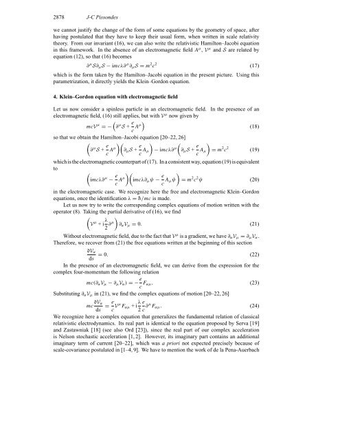
2878 J-C Pisson<strong>de</strong>s<br />
we cannot justify the change of the form of some equations by the geometry of space, after<br />
having postulated that they have to keep their usual form, when written in scale relativity<br />
theory. From our invariant (16), we can also write the relativistic Hamilton–Jacobi equation<br />
in this framework. In the absence of an electromagnetic field A µ , V µ and S are related by<br />
equation (12), so that (16) becomes<br />
(17)<br />
which is the form taken by the Hamilton–Jacobi equation in the present picture. Using this<br />
parametrization, it directly yields the Klein–Gordon equation.<br />
∂ µ S∂µS − imcλ∂ µ ∂µS = m 2 c 2<br />
4. Klein–Gordon equation with electromagnetic field<br />
Let us now consi<strong>de</strong>r a spinless particle in an electromagnetic field. In the presence of an<br />
electromagnetic field, (16) still applies, but with V µ now given by<br />
mcV µ <br />
=− ∂ µ S+ e<br />
c Aµ<br />
(18)<br />
so that we obtain the Hamilton–Jacobi equation [20–22, 26]<br />
<br />
∂ µ S + e<br />
c Aµ<br />
<br />
∂µS + e<br />
c Aµ<br />
<br />
− imcλ∂ µ<br />
<br />
∂µS + e<br />
c Aµ<br />
<br />
= m 2 c 2<br />
(19)<br />
which is the electromagnetic counterpart of (17). In a consistent way, equation (19) is equivalent<br />
to<br />
<br />
imcλ∂ µ − e<br />
c Aµ<br />
<br />
imcλ∂µψ − e<br />
c Aµψ<br />
<br />
= m 2 c 2 ψ (20)<br />
in the electromagnetic case. We recognize here the free and electromagnetic Klein–Gordon<br />
equations, once the i<strong>de</strong>ntification λ = ¯h/mc is ma<strong>de</strong>.<br />
Let us now try to write the corresponding complex equations of motion written with the<br />
operator (8). Taking the partial <strong>de</strong>rivative of (16), we find<br />
<br />
V µ +i λ<br />
2 ∂µ<br />
<br />
∂αVµ =0. (21)<br />
Without electromagnetic field, due to the fact that V µ is a gradient, we have ∂αVµ = ∂µVα.<br />
Therefore, we recover from (21) the free equations written at the beginning of this section<br />
dVα<br />
= 0. (22)<br />
ds<br />
In the presence of an electromagnetic field, we can <strong>de</strong>rive from the expression for the<br />
complex four-momentum the following relation<br />
mc(∂αVµ − ∂µVα) =− e<br />
c Fαµ. (23)<br />
Substituting ∂αVµ in (21), we find the complex equations of motion [20–22, 26]<br />
mc dVα e<br />
=<br />
ds c Vµ Fαµ +i λe<br />
2c<br />
∂µ Fαµ. (24)<br />
We recognize here a complex equation that generalizes the fundamental relation of classical<br />
relativistic electrodynamics. Its real part is i<strong>de</strong>ntical to the equation proposed by Serva [19]<br />
and Zastawniak [18] (see also Ord [23]), since the real part of our complex acceleration<br />
is Nelson stochastic acceleration [1, 2]. However, its imaginary part contains an additional<br />
imaginary term of current [20–22], which was a priori not expected precisely because of<br />
scale-covariance postulated in [1–4, 9]. We have to mention the work of <strong>de</strong> la Pena-Auerbach