PDF file: 2.9 Mbytes - Laboratoire de Physique des Hautes Energies ...

Searching for Higgs decays
to four bottom quarks
at LHCb
Master Thesis
Julien Rouvinet
Laboratoire de Physique des Hautes Energies
Faculté des Sciences de Base
Ecole Polytechnique Fédérale de Lausanne
Jury
Professeur Aurelio Bay, directeur du travail
Expert externe : Victor Coco
Lausanne 2009-2010

Abstract
In a recent paper[1], David E. Kaplan and Matthew McEvoy have claimed that it will
be possible to detect the Higgs boson in the LHCb experiment if its main decay occurs
through the channel h 0 → aa → b ¯ bb ¯ b for a Higgs mass not too far above current limits.
Many models beyond the Standard Model, like NMSSM 1 , little Higgs, composite Higgs
or any model where new light scalar (or pseudo-scalar) particles are coupled to the Higgs
incorporate such phenomenology. The main feature of the LHCb experiment is the reconstruction
of b particles through a proper b-tagging. The goal of this Master Thesis is to
test this hypothesis through a preliminary study of this particular Higgs decay mode using
Pythia. A background contribution is generated using Alpgen. b-jets are reconstructed
in order to recover the pseudo-scalar particle a. Two a candidates are subsequently combined
to obtain the Higgs. Finally, a Toy Monte Carlo is made to asses the capability to
extract the signal.
1 Next-to-Minimal SuperSymmetric Standard Model

Contents
1 The Large Hadron Collider and The LHCb experiment 5
1.1 The LHC . . . . . . . . . . . . . . . . . . . . . . . . . . . . . . . . . . . . . 5
1.2 The LHCb Experiment . . . . . . . . . . . . . . . . . . . . . . . . . . . . . . 6
2 Theoretical overview 9
2.1 Standard Model and Higgs Boson . . . . . . . . . . . . . . . . . . . . . . . . 9
2.1.1 The Standard Model . . . . . . . . . . . . . . . . . . . . . . . . . . . 9
2.1.2 The Higgs Mechanism . . . . . . . . . . . . . . . . . . . . . . . . . . 10
2.2 The Higgs to four b decay . . . . . . . . . . . . . . . . . . . . . . . . . . . . 11
2.2.1 QCD backgrounds to h 0 → aa → b ¯ bb ¯ b . . . . . . . . . . . . . . . . . 11
3 Events generation using Pythia and Alpgen 13
3.1 Generation of signal events using Pythia . . . . . . . . . . . . . . . . . . . 13
3.2 Background contributions using Alpgen . . . . . . . . . . . . . . . . . . . . 15
3.3 Number of generated events . . . . . . . . . . . . . . . . . . . . . . . . . . 16
3.4 MC-events generation and analysis . . . . . . . . . . . . . . . . . . . . . . . 16
4 Study of the h 0 → aa → b ¯ bb ¯ b signature in LHCb 19
4.1 b quarks analysis . . . . . . . . . . . . . . . . . . . . . . . . . . . . . . . . . 19
4.2 Jets reconstruction . . . . . . . . . . . . . . . . . . . . . . . . . . . . . . . . 21
4.3 Reconstruction of the a . . . . . . . . . . . . . . . . . . . . . . . . . . . . . 26
4.3.1 Selection cuts . . . . . . . . . . . . . . . . . . . . . . . . . . . . . . . 27
4.4 Higgs reconstruction . . . . . . . . . . . . . . . . . . . . . . . . . . . . . . . 30
4.5 Number of events . . . . . . . . . . . . . . . . . . . . . . . . . . . . . . . . . 31
4.6 Muons plots . . . . . . . . . . . . . . . . . . . . . . . . . . . . . . . . . . . . 32
4.7 Extraction of the signal: a Toy Monte-Carlo study . . . . . . . . . . . . . . 34
4.7.1 A statistical enhancement trick . . . . . . . . . . . . . . . . . . . . . 34
4.7.2 TMC results . . . . . . . . . . . . . . . . . . . . . . . . . . . . . . . 35
5 Conclusion 39
A Alpgen parameters 41
B Other plots 43
3

Chapter 1
The Large Hadron Collider and
The LHCb experiment
1.1 The LHC
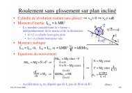
Figure 1.1: The Large Hadron Collider and its associated experiments
The LHC is the CERN’s 1 new circular hadrons collider located beneath the Franco-
Swiss border near Geneva Switzerland. It has been commissioned on autumn 2008 and
reopened on November 2009 after some adjustments. This collider is the world’s largest
and highest-energy particles accelerator. It lies in a tunnel of 27 km of circumference and
will produce collisions between protons at an energy of 7 T eV in the center of mass frame
and between P b ions at an energy of 574 T eV per nucleus. The most famous question
which is likely to be answered through this incredibly technical challenge concerns the
existence and properties of the Higgs boson. Physicists are also looking for an explanation
of the imbalance between matter and antimatter in the Universe. Moreover, because of
the huge available energy, new types of particles (for instance SUSY’s) may be produced.
Properties of the quark-gluon plasma will also be hunted down. Therefore, to perform
these crucial break-throughs, four major experiments have been installed along the cave.
1 Centre Européen pour la Recherche Nucléaire: international collaboration created in 1954
5

ATLAS, A Toroidal LHC ApparatuS, is designed to observe phenomena involving
massive particles, in particular the electroweak interaction symmetry breaking through
the Higgs mechanism. It might shed light on theories beyond the Standard Model. This
five stories sized detector is designed to measure the broadest range of energy signals
rather than focusing on a specific process.
The second experiment is CMS, the Compact Muon Solenoid. It also is a general
purpose detector designed with the same goals than ATLAS. These two detectors will
complement each other, hopefully finding new physics and discovering the Higgs boson.
The third one is ALICE, A Large Ion Collider Experiment. It will study P b − P b
collisions in order to investigate the quark gluon plasma. This state of matter is supposed
to have been generated close to the Big Bang.
Finally, the LHCb, Large Hadron Collider beauty, is designed to understand the
matter-antimatter asymmetry through the study of CP violation in B-mesons systems.
More details are given on the next section.
1.2 The LHCb Experiment
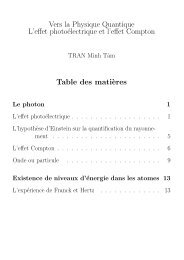
Figure 1.2: The LHCb experiment in the vertical plane
The LHCb is a single arm forward spectrometer with an angular coverage (acceptance)
of 15 < θ < 330 mrad corresponding to a pseudo rapidity of 1.8 < η < 4.9 where
η = −ln(tan(θ/2)). This angle seems small but is justified by the fact that b-hadrons
have a transverse momentum smaller than their longitudinal momentum. The detector is
optimized to exploit the large number of b quarks produced during the collision. The LHCb
luminosity is lower than the luminosity potential of the LHC. It is set to L LHCb = 2 · 10 32
cm −2 s −1 to obtain an average of one p−p interaction per crossing. We can notice different
components:
6

• The Vertex Locator (VELO): Surrounding the interaction point, it is made of 25
silicon stations of 200 µm of thickness. The VELO allows the reconstruction of the
position of the secondary vertices with a resolution of about 300 µm.
• RICH1 and RICH2: These two Ring Imaging Cherenkov detectors allow particles
identifications.
• TT, T1, T2 and T3 trackers: measure the momentum of charged particles deviated
by a magnetic field.
• The Scintillator Pad Detector (SPD): differentiates charged particles from neutral
ones.
• The PreShower (PS): It achieves the pre-detection of electromagnetic showers and
distinguishes between electrons and pions.
• The ECAL and HCAL: These two calorimeters measure the total amount of energy
deposed by the electrons, photons and hadrons.
• The M1-M5 Muons detector: Positioned at the end of the detector, they measure
the total energy of muons, particles weakly interacting.
Once the collisions start, it is important to select the events to store because if everything
was to be saved, the amount of data would be of the order of 40 T B/s. To achieve
the reduction, two stages of trigger are performed. The first level is interesting because it
makes the study of the Higgs decay into four b quarks worth at LHCb. The Level-0 Trigger
is based on calorimeter and muon chamber information in order to reduce the event rate
down to 1 MHz by requiring a muon, an electron, a photon or a hadron with an high
transverse momentum and transverse energy. Tracks associated with b-hadron decays fulfill
these conditions. Also, in inclusive production, the Higgs is significantly boosted along
the z-axis and thus, at least one b quark often lives at large pseudo-rapidity, and therefore
excellent tracking and vertexing in the forward region are crucial for the kind of signal we
are interested in[1].
More details on the LHCb experiment and on the trigger system can be found on its
internet website or in [3].
7

Chapter 2
Theoretical overview
This chapter consists in a very brief presentation of the Standard Model of particles physics
along with a quick introduction to the Higgs mechanism. Plenty of good books can be
consulted on these subjects. Therefore, only the material useful for this work is described.
2.1 Standard Model and Higgs Boson
2.1.1 The Standard Model
The Standard Model of particle physics (or SM) is a relativistic quantum field theory which
describes three of the four fundamental interactions of Nature and the elementary particles
that undergo these interactions. This model is a gauge theory which is in relatively good
agreement with the present (beginning of 2010) experimental results. The SM gauge group
is:
Electro−weak interaction
GSM = SU(3)c
× SU(2) × U(1)
Strong interaction (color)
SU(3)c is the group associated with Quantum Chromo Dynamics (the subscript c
stands for color, which is the name of the strong charge) while SU(2) × U(1) is associated
with both the electromagnetic and weak forces. The model also describes the elementary
particles. A list of those particles and their masses is given in Figure 2.1.
9

Leptons
Quarks
Particle Mass [MeV/c 2 ]
e - 0.511
! e

2.2 The Higgs to four b decay
Assuming that the SM is correct up to 1 T eV , we know quite well the production cross
section and the decay width of the Higgs for any given mass. Nevertheless, these quantities
are very sensitive to the physics hidden beyond the SM. If we assume the existence of a
light neutral pseudo scalar particle having a mass about half the Higgs mass, the Higgs
could decay dominantly into this particle without affecting the Z width too much. This
particle will be called a through all this work. Many models include such phenomenology.
Let us name for example the NMSSM, Higgs composite and little Higgs theories. We will
assume that the branching ratio of the Higgs to the a is equal to one and that the a is
forced to decay into a b − ¯ b pair. The large number of models containing this physics can
be approximated simply by adding this a to the SM. The coupling to the Higgs is then
simply:
This term will generated a mass given by:
1
2 λa2 H † H (2.1)
m 2 a = 1
2 λv2
(2.2)
v 246 GeV being the Higgs vacuum expectation value. The decay rate for this process
is:
Γ(h → aa) 1
32π
λ 2 v 2
mh
1 − 4m2 a
m 2 h
(2.3)
This width dominates the Higgs decay comparing to the total decay rate of a (e.g. 115
GeV ) SM Higgs if the coupling to the scalar is λ > 0.25 1 .
2.2.1 QCD backgrounds to h 0 → aa → b ¯ bb ¯ b
In addition to the signal, we have to consider the existence of an irreducible QCD b ¯ bb ¯ b
background because these four b could be mistaken as resulting from a decays. Hence, it
is necessary to include those b to the study.
We must also include a b ¯ bt¯t component because the top quark usually decays into a b
quark which will give birth to another source of background. However, it appears that
this source is negligible, because its production cross section 2 is small (as is illustrated in
table 4.1).
Another source of background is related to the limited capability to discriminate between b
and c jets. The LHCb experiment is designed to recognize b events, this is called b-tagging.
Nevertheless, the efficiency of b-tagging is not 100%. Sometimes, c jets are mistaken to be
b jets. In a recent paper (see ref.[5]), A.Bay and C. Potterat describe an algorithm for the
determination of the seeds to be used in the reconstruction of b jets. They show that the
typical efficiency to discover b jets is about 70%. The probability to confuse c with b jets
is about 30%. Enhanced flavour criteria will be considered in further studies to improve
those efficiencies. Taking this fact into consideration leads us to add a b ¯ bc¯c background
contribution to our analysis.
1 see [1] from which this section is strongly inspired
2 The cross section given by Alpgen for this process is 3, 78 pb.
11

V ∗
V ∗
Chapter 3
Events generation using Pythia
and Alpgen
To study the Higgs decay into four b-quarks, the standalone computer program Pythia
version 6.325 is used. We have chosen this version to insure compatibility with Alpgen
version 2.13, which is a generator for hard multiparton processes in hadronic collisions[4].
These two generators are based on Monte Carlo methods. The energy in the center of
mass frame of the two incoming protons is √ s = 14 T eV , corresponding to the maximal
energy that should be reached by the LHC at the end of the year 2012.
3.1 Generation of signal events using Pythia
The various and most important parameters used to generate signal events are described
here. First, the decay file used by Pythia has to be modified in order to force the Higgs to
turn into two a particles. Then, each a has to decay into a b−¯b pair. Therefore, a new bloc
is added in the decay file, corresponding to the a (associated to the identification number
σh0 pbarn → 5.9 · 10
n°35). The branching ratio for the decay of a into four b-quarks is set equal to one. For
the Higgs decay into two a, the branching ratio is set to 0.97 because the inverse process
of the gluons fusion used to generate the Higgs has to be permitted. The Higgs mass and
5
σbb 2.45 · 108 pbarn → 1.5 · 1012 σZW 4.33 · 106 pbarn → 2.7 · 10 10
the a mass are both parameters. We will vary them to see how the kinematics changes.
σtt 2.75 · 103 pbarn → 1.7 · 107 b/t
q
h 0
q
q
h 0
q
We have considered two different masses for the Higgs: mh = 115 and 125 GeV c −2 and
three different masses for a: ma = 20, 25 and 35 GeV c −2 . This is made by changing the
masses in the decay file used by the program.
The Higgs boson is produced by Pythia through gluons fusion 1 . The associated Feynman
diagram is shown in Figure 3.1.
g q
h 0
g q
q
q
V ∗
b/t
V
1 by setting MSUB(102) = 1
h 0
g q
q
g q
q
gg
Figure 3.1: Feynman diagram of gluons fusion
q
q q
13
h 0
h 0

After production, the program computes the hadronization and the decay processes of
the event. An example of event can be found in [3].
The most relevant configuration parameters used for the simulation are given in table
3.1.
Parameter Value Explanation
MSTP(2) 2 Compute αs to second order
MSTP(61) 1 QED and QCD initial state radiation
MSTP(71) 1 QED and QCD final state radiation
MSTP(81) 1 Multiple interactions
MSTP(82) 3 Structure of multiple interactions
MSTP(111) 1 Fragmentation and decay
MSTP(131) 0 Only one event is generated at a time
MSTP(151) 1 Program execution
MSTU(21) 1 Check on possible errors during program execution
PARP(67) 1.0 ·Q 2 : maximum parton virtuality allowed in time-like showers
PARP(81) 21 Effective min. transverse momentum p⊥min for multiple interactions
PARP(82) 4.50 Regularization scale p⊥0 for multiple interactions
PARP(85) 0.33 Related to gluons in multiple interactions
PARP(86) 0.66 Related to gluons in multiple interactions
PARP(89) 14000.0 Reference energy scale
PARP(90) 0.116 Power of the energy-rescaling term of the p⊥min and p⊥0 parameters
PARP(91) = 1.0 Width of Gaussian primordial k⊥ distribution inside hadron
PARP(131) 0.0048 Luminosity for pile-up events
PARP(151) 0.007 [mm] σx of beam
PARP(152) 0.007 [mm] σy of beam
PARP(153) 0.059 [mm] σz of beam
PARP(154) 0 [mm/c] σt of beam
MSTJ(1) 1 String fragmentation according to the Lund model
MSTJ(26) 0 No B– ¯ B mixing in decays.
PARJ(11) 0.5 Prob. spin 1 light meson (containing u and d quarks only)
PARJ(12) 0.4 Prob. spin 1 strange meson
PARJ(13) 0.79 Prob. spin 1 charm or heavier meson
PARJ(14) 0.0 Prob. spin 0 meson is prod. with orb. ang. mom. 1, for total spin 1
PARJ(15) 0.018 Related to probability of specific meson production
PARJ(16) 0.054 Related to probability of specific meson production
PARJ(17) 0.131 Related to probability of specific meson production
PARJ(33) 0.4 Define the remaining energy below which 2 final hadrons are formed
Table 3.1: Most important configuration parameters used in Pythia. These parameters
are directly implemented into the Fortran code. For more details on the list of parameters
and on their usage see [8].
14

3.2 Background contributions using Alpgen
Alpgen [4] is dedicated to the study of multiparton hard processes in hadronic collisions.
It is based on the ALPHA algorithm. Therefore, it constitutes the perfect tool to generated
b ¯ bb ¯ b, b ¯ bc¯c and b ¯ bt¯t backgrounds. The generation is divided into two phases. The first
one produces weighted events whereas the second produces the unweighted events that
will be showered through Pythia. The first phase is initialized by a file containing the
informations given in table 3.2. An example of file is given in Appendix A.
Parameter and explanation Value
imode, 1 generates weighted events and writes to file for later unweighting 1
Label for the produced files bbbb
Grid: The generator will use a new grid 0
Number of events per iteration and number of warm-up iterations 100000000 2
Number of events generated after warm-up 100000000
ihvy: choose the heavy flavour type, here b quark 5
ihvy2: same as before to insure b ¯ bb ¯ b production 5
ebeam: beam energy in the center of mass frame 7000.0
ih2: Select pp collisions 1
ndns: Parton density function, CTEQ5L * is used 5
njets: Number of light jets 0
etabmax: Pseudo rapidity η maximum of b quarks 4.5
drbmin: ∆R minimum between b quarks 0.1
ptbmin: Minimum transverse momentum of b quarks 10
Table 3.2: Chosen parameters for the first generation phase in Alpgen. These are the
parameters for the b ¯ bb ¯ b component of the background leading to 703 ′ 906 events generated.
For a complete list and more explanations see [4] and [9]. The parameters for the b ¯ bc¯c
and b ¯ bt¯t components are given in Appendix A.
After the first phase, weighted events are produced. The program subsequently can
perform the unweighting of those events. The names of the weighted files are also used
for the names of the output files. Those files are:
• qqqq.stat: Contains value of the input parameters, list of hard process selected
and generation cuts. It then reports the results of each individual integration cycle,
with total cross sections and individual contributions from the allowed subprocesses.
Contains maximum weights of the various iterations, the corresponding unweighting
efficiencies, and the value of the cross-section accumulated over the various iterations
weighted by the respective statistical errors.
• qqqq.grid1 and qqqq.grid2: The phase-space is discretized and parameterized
by a multi-dimensional grid. Those files contain details on the grid and on its
parametrization.
• qqqq.par and qqqq unw.par: Include run parameters (beam energies and types,
generation cuts, etc), phase-space grids, cross-section and maximum-weight information.
15

• qqqq.wgt: Stores the two seeds of the random number generation, the event weight
and the value of other parameters of the event.
• qqqq unw.stat: Includes cross sections, maximum weight, etc...
• qqqq.unw: List of unweighted events, including event kinematics, flavor and color
structure and event weight.
Finally, these events are transfered to Pythia via the qqqq unw.par and qqqq.unw
files.
3.3 Number of generated events
We have produced 10 ′ 000 signal events. 700 ′ 000 b ¯ bb ¯ b background events and 500 ′ 000 b ¯ bc¯c
background events have been treated with Pythia after generation by Alpgen.
3.4 MC-events generation and analysis
Once the events are generated, the program should be capable to sort the particles, perform
some treatments like jet reconstructions and store the interesting informations in files that
can be used for further analysis. In this section, the different algorithms used to study
the characteristics of both the signal and the background are enumerated and briefly
presented.
Events generation
The program written for this work 2 offers two different options. The first one is the
generation of signal events that can be stored or directly treated by various algorithms.
It manages the interface with Pythia and the selection of the decay file. The program
checks that h → aa events have been produced and counts these events for statistical
purposes.
The second option passes the background events produced by Alpgen to Pythia for
hadronization.
Acceptance
The LHCb experiment has a limited angular coverage implemented in the code by checking
that every interesting particle belongs to the cone defined by:
15 < θ < 390 mrad (3.1)
which is a little bit bigger than the LHCb acceptance to allow for boundary effects studies
in further analysis. This condition implies that only particles lying inside the cone are
considered.
2 in the FORTRAN language (see [7])
16

Searching the muons and their genealogy
In the article [1] on which this analysis is inspired, the LHCb experiment is chosen because
of its inclusive muon trigger which acts as an ”existence proof” to save the data to disc.
Therefore, the program looks for muons and checks if they are products of the decay of
a b-hadron, coming from the decay product of one a. Then, a consistency check is made
by verifying that the inclusive branching ratio of b hadrons to muons is about 11%. It
is indeed the case for every simulation we made. Finally, informations are stored and
statistics are computed.
Jet reconstruction
Each of the b quarks produced is used as a seed for the jet reconstruction. Of course, in
real life, the b quarks are not directly observable and it is only through jet reconstruction
that information on the Higgs and a masses can be gathered. The code contains different
algorithms for the reconstruction. Details will be given in the chapter 4.
Saving the informations
All important data are saved in (.hbk) files that can be analyzed later 3 . We construct
histograms of the kinematical variables of jets, b quarks, muons, a and Higgs. The energy
and momentum are saved along with different sets of variables as the angular distance
between particles. It is also possible to store the full event generations in (.dat) files that
can be read later for analysis.
The mismatch algorithm
This simple algorithm is the implementation of the possibility that the detector misinterprets
a c quark to be a b quark. A b quark has roughly 70% of chance to be correctly
recognized. A c quark has a probability of 30% to be interpreted as a b quark. This fact is
explained in [5], which describes a preliminary study of an algorithm allowing b jet reconstruction.
Researches are being made on this subject and progresses are expected, leading
to a better reconstruction and therefore reducing the impact of the b ¯ bc¯c background considered
here.
In practice, the algorithm overwrites the identification number of the c quarks (from 4 to
5), leading the program to consider c jets as b ones. The possibility to mix up the c and
b quarks is offered at the beginning of the treatment of the background.
3 using either Paw or Root; these two programs enable histograms and statistical treatments of data
17

Chapter 4
Study of the h 0 → aa → b ¯ bb ¯ b
signature in LHCb
This chapter describes the signature of the h0 → aa → b¯bb¯b physical process as well as
the contribution of different backgrounds. It also proposes a Toy Monte Carlo analysis to
study the efficiency of the signal detection. For the analysis, we choose mh = 115 GeV/c2 and ma = 20 GeV/c2 . We have also generated events with mh = 125 and ma = 25 and
35 GeV/c2 . For those cases, the analysis is essentially the same, therefore, only the first
set of parameters is fully described here. To follow the work presented in [1], it would be
interesting to complete the study for those different masses too and see the effect of their
variations on the efficiency of the method illustrated in what follows.
The b quarks hadronize into ”jets”. A technique to reconstruct jets is based on the cone
algorithm: particles are gathered when they fall inside a cone of aperture ∆R in (η, φ)
space 1 . The angular distance is defined by Eq. 4.1.
∆Rij = (ηi − ηj) 2 + (φi − φj) 2 (4.1)
For simplicity, we consider events where the four b quarks are either produced by the
signal or by background contributions. Mixed possibilities where, for instance, a b is the
result of another process and the three others are signal ones are not discussed. Of course,
these more complicated situations have to be considered in further studies.
In the following, the signal and background distributions are normalized to 1 unless
otherwise is specified.
4.1 b quarks analysis
We first consider the kinematics of the b quarks. Only events with four b quarks inside the
LHCb acceptance are considered 2 . This corresponds to about 7% of the generated signal
events and 3.5% of b ¯ bb ¯ b and b ¯ bc¯c generated background events.
First, the angle and ∆R distributions are represented in order to find a good strategy
to reconstruct jets. Obviously, if the b are produced close to each other, their jets will
overlap and it will be difficult to reconstruct them. Figure 4.1 shows the angular and
∆R distributions of the b of the signal and also of the b coming from the b ¯ bb ¯ b and b ¯ bc¯c
backgrounds. A jet is generally constructed with a cone radius of Rcone = 0.6. Therefore,
1 See Ref.[2] and [5]
2 Let us recall that the enlarged acceptance is 15 < θ < 390 mrad
19

two jets overlap if ∆R(b1, b2) < 2 · Rcone = 1.2. The ∆R distance for the signal is less
than one suggesting that the jets are likely overlapping each other. The background
distributions are flatter, especially for b ¯ bb ¯ b. That is why it is difficult to reconstruct each
jet for the signal. Another strategy must be adopted.
Figure 4.1: Angle and ∆R between the b from the signal (black), the b ¯ bb ¯ b background
(red) and the b ¯ bc¯c (blue) background. We note that the ∆R background distribution is
much flatter than the signal distribution. The small ∆R distance indicates that some jets
overlap.
Figure 4.2 shows the transverse momentum distribution of the b quarks coming from
signal and backgrounds. The Pt distribution of the signal is wider than those of the
backgrounds and the average Pt is smaller.
20

Figure 4.2: Pt of b quarks from the signal (black), the b ¯ bb ¯ b background (red) and the b ¯ bc¯c
background (blue).
4.2 Jets reconstruction
Our objective is to reconstruct the mass of the a and of the Higgs. The four jets will
consequently be combined. Therefore, it is not necessary to reconstruct each of them to
match the ”real” physical jets. Section 4.1 brings to light the possibility for the real jets
to overlap.
What we do is to use each b quark as a seed and, to avoid multiple particle counting,
group the b in pairs corresponding to a candidate . Then, for each particle of the list, we
test if it belongs to the cone of maximal radius ∆R = 0.6 centered around the first quark.
If it is not the case, we test the condition for the second quark. Of course, in the case of
two jets overlapping, the first reconstructed jet will contain more particles than the other
one. Nevertheless, because we combine those two jets to reconstruct the a candidate, it
does not matter. The only trick we have to do is to decide how to form the pairs of b used,
out of the three different combinations we can do. The solution that will be adopted is
explained in the section 4.3.
Quarks are not directly observable in practice, therefore, it would have been more realistic
to use b-hadrons instead of b quarks as seeds. However, because the ∆R distance between
21

Figure 4.3: For each event with 4 b quarks inside the acceptance, ∆Rmin and ∆Rmax
between pairs of b are computed. Those plots show evidences of future jets overlapping.
the quark and the corresponding b-hadron is small (〈∆R〉 0.02, see ref.[2]), using the
quark is justified.
22

Figure 4.4: Transverse momentum of two of the four b jets from the signal (top) and the
b ¯ bb ¯ b background (bottom).
23

Figure 4.5: Transverse momentum of two of the four b jets from the signal (top) and the
b ¯ bb ¯ b background (bottom).
Figures 4.4 and 4.5 illustrate the four jets Pt obtained from our algorithm. Pt(ji) is
the transverse momentum of the jet number i. i = 1, 3 correspond to the two ”biggest”
jets while i = 2, 4 are the two ”smallest” (see Figure 4.4 and 4.5). j1 and j3 have wider
spectra because they contain more particles, being built from the first seeds. Looking at
those graphs, it is impossible for us to already determine selection cuts to discriminate
between b ¯ bb ¯ b QCD background and signal, except a possible lower cut around 20 GeV/c
for Pt of j1 and j3.
To have a better understanding of the situation, we can make a correlation plot of the
transverse momentum of jets. This is done for a particular combination (jet 1 with jet
2 and jet 3 with jet 4) in figure 4.6. We see a more pronounced anti-correlation for the
signal than for the background.
24

Figure 4.6: Transverse momentum of the b quarks of the signal (top) and the b ¯ bb ¯ b background
(bottom).
25

4.3 Reconstruction of the a
From the Monte Carlo truth, we can calculate the production angle and ∆R between two
a as shown in Figure 4.7.
Figure 4.7: Angle and ∆R between the a obtained from MC truth.
We see that the a are produced well separated from each other with ∆R peaked at 3.
The main problem is to choose the most likely two combinations of 2-jets out of the three
possibilities.
The first criteria tested was the combination of the two jets whose seeds are the closest.
We computed the ∆R distance between all the b and combined the two nearest b together.
The two b left form the second a candidate.
Another criteria is suggested in [1]. It consists in choosing the combination which minimizes
the quantity (R1) 2 + (R2) 2 , where R1 (R2) is the distance between the first (second)
pair of jets.
For our quadrivector analysis, no significant differences appear between the two methods
for signal events. Therefore, we have chosen to use the first method by combining the jets
with the closer seeds. A comparison graph of the two methods is available is Appendix
26

B. We have also computed the percentage of correct combinations by checking that the
combined jets are those with the seeds that come from the same a (using the Monte Carlo
truth). We found about 99 % of correct combinations 3 .
4.3.1 Selection cuts
Selection cuts are conditions imposed on different observables or their combinations to
improve the discrimination between signal and background. The discrimination power is
evaluated from the ratio :
which is called ”significance”.
σ = S/ √ S + B (4.2)
Figure 4.8: Transverse momentum of the two a candidates for signal (black) and b ¯ bb ¯ b
background (red). The third plot shows the correlation between Pt(a1) and Pt(a2). (Plots
displaying the b ¯ bc¯c background are showed in Appendix B.)
Figure 4.8 shows the transverse momentum of both the signal and the b ¯ bb ¯ b background.
It suggests to cut at about 40 GeV c −1 to get rid of a large part of the background. The
third plot strongly suggests to cut rather on the anti-diagonal, at Pt1 + Pt2 = 70 GeV c−1 .
Unfortunately, doing so would imply a strong bias on the unknown Higgs mass. Thus, a
3 This percentage is strongly dependent on the mass parameters used for the generation. For instance
with mh = 125 GeV and ma = 35 GeV we found 73% of correct combinations.
27

weaker condition is chosen:
Pt(j1) + Pt(j2) < 60 GeV c −1
Pt(j3) + Pt(j4) > 20 GeV c −1
(4.3)
Figure 4.9 shows the masses of the a candidates (and also the reconstructed Higgs
mass). No cut has been imposed yet. The distributions suggest to introduce:
13 < ma < 25 GeV c −2
(4.4)
Applying the cuts 4.3 we obtain Figure 4.10. The green arrows represent the cuts given
by 4.4.
28

Figure 4.9: Reconstructions of the mass of the a candidates obtained from the signal and
the backgrounds (b ¯ bb ¯ b in red top three plots and b ¯ bc¯c in blue bottom three plots). No cuts
are applied yet.
We observe that the mass of the reconstructed a is smaller than the value used for the
simulation (ie 20 GeV c −2 ). This is due to the loss of neutrini in jets reconstruction along
with the loss of particles produced outside the acceptance.
29

Figure 4.10: Reconstructed mass distributions of the two a after cuts. b ¯ bb ¯ b background is
represented in red while b ¯ bc¯c is in blue. The green arrows symbolize the mass cuts given
by Eq. 4.4
4.4 Higgs reconstruction
We can now combine the two a candidates to get the mass distribution for the Higgs boson
candidate.
Figure 4.11 shows that the reconstructed Higgs mass is smaller than the mass used for
generation (115 GeV c −2 ). This is explained by the same argument as for the ma. The
30

Figure 4.11: Higgs mass reconstructions. As usual, b ¯ bb ¯ b background is in red and b ¯ bc¯c is
in blue.The number of events corresponds to our Monte Carlo sets.
mass values obtained from both backgrounds are even smaller. A fitting method to extract
the signal from the signal plus background distribution will be discussed in section 4.7.
4.5 Number of events
We can compute the number of events expected per year by using the formula:
Nevts =
LLHCb dt · [σ h 0 · BR(h 0 → aa) · BR(a → b ¯ b) 2 ] (4.5)
The luminosity integrated over a running year of the LHCb is equal to 2 fb −1 . The
branching ratios are set to be equal to one because of theoretical arguments given in
Chapter 2. We also multiply Eq. 4.5 by the percentage of events lying in the enlarged
LHCb acceptance.
31

Using the total number of events and the number of events that pass the cuts, we can
compute the values in Table 4.1.
Cross % Total number Prob. of 4 b’s Number
Process section in of events after recognition passing the cuts
σ [pb] accept. 1 LHCb year ɛb ×ɛb
Higgs production 94 7.5 1.4 ·10 4 (0.7) 4 1.9 · 10 3
b ¯ bb ¯ b background 19661.5 3.5 1.38 · 10 6 (0.7) 4 5.75 · 10 4
b ¯ bc¯c background 52053.3 3.5 3.67 · 10 6 (0.7) 2 · (0.3) 2 3.3 · 10 4
b ¯ bt¯t background 3.78 0.55 41.8 (0.7) 4 6.2 · 10 −2
Table 4.1: Cross sections and number of events per year for signal and backgrounds. This
table clearly shows that b ¯ bt¯t can be neglected.
The cross section for signal events is an estimation for Higgs production with a mass
around 120 GeV in the MSSM (see Ref.[3]), assuming that the branching ratio to four b
is equal to one. An analysis of the effect of the variation of the number of events is made
in Section 4.7. The background cross section are computed by Alpgen. We clearly see
that the b ¯ bt¯t background contribution is negligible because its cross section is small and
nearly none of them actually passes the cuts. The fourth column is the expression of the
fact that the detector will not recognize correctly every b jet as explained in 2.2.1.
4.6 Muons plots
For completeness, we shall take a look at the muon decay of the b-hadrons, as suggested
in [1], where the LHCb muon trigger is described as an advantage for our study. Figure
4.12 shows the transverse momentum distributions of the muons produced by the collision.
The good muons are the ones directly coming from the decay chain of an a. We can see
that the Pt is a little bit smaller for the good muons but the difference is too small to have
a real signification. The shapes of the distributions are approximately the same.
32

Figure 4.12: Transverse momentum of the muons directly coming from the decay chain
of an a (top) and of all the muons (bottom).
For an event to be saved, the LHCb L0 trigger needs to detect, among other things, a
muon with a Pt > 1.1 GeV . This could lead to the imposition of another cut which will
decrease the number of events waited per year.
It is interesting to notice that only 389 signal events over the 10 ′ 000 generated contain
muons. Besides, only 745 signal events have produced 4 b quarks inside the (enlarged)
acceptance. Among those events, 327 contain at least one muon inside the acceptance
with a Pt > 1.1 GeV . Therefore, if we trigger the production of 4 b quarks (from the
signal) inside the acceptance with muons, the efficiency is about 44%, meaning that 44%
of the signal events producing 4 b inside the acceptance will actually be saved to disk. The
percentage is roughly the same (about 35%) for both types of background events.
33

4.7 Extraction of the signal: a Toy Monte-Carlo study
The Toy Monte Carlo (TMC) procedure is a method to test the sensibility of our analysis
to the variation of the number of signal events. Indeed, the number of signal events varies
according to the model considered along with the mass of the a and of the Higgs.
The TMC method is used to simulate many ”LHCb experiments”. For each of those
”experiments”, we randomly generate a number of signal events, keeping the background
at the average value (plus statistical variations). The number of signal events is changed
from 1/10 to 3 times the number of events per year seen before. We reproduce 100
experiments for each value of signal and background events. The Higgs mass is fixed for
this procedure and the shape of the background is supposed to be known. In reality, when
dealing with experimental data, a scan is made on the Higgs mass. Here, a fit of signal
plus background is perform by the Minuit algorithm (without normalization of the total
number of events). The goal is to determine the efficiency of the signal extraction from
this fit. The significance depends on the number of signal events used for the fit.
4.7.1 A statistical enhancement trick
We have generated 5 ′ 000 signal events for this analysis. Only 385 of these events contain
four b quarks inside the LHCb acceptance. Applying the cuts (see equations 4.3 and
4.4), only 217 events remain. This number roughly corresponds to 1
10 of a running year of
LHCb. It would be interesting to increase this number of events for the TMC analysis4 . An
obvious way to do that would have been to generate more events, but the time needed to
generate enough events is long. Therefore, we use another way to ”increase” the statistics
by smoothing the curves used for the TMC. Doing so, we do loose some information but
the global shape of the distributions remains the same. This approach is quite conservative
because the smoothing could only destroy some specificity of the curves that would have
been useful for discrimination. The effect of smoothing can be seen in figure 4.13.
Thanks to this procedure, we assume that we have gained about one order of magnitude
in statistics.
year.
4 for our simulated ”experiments” to correspond to a time around ten times longer, ie about 1 running
34

Figure 4.13: Effect of the smearing realized to mimic a higher number of events for the Toy
Monte Carlo. The curves are smoothed. Top: original distributions. Middle: smoothed
distributions. Bottom: negative values suppressed.
4.7.2 TMC results
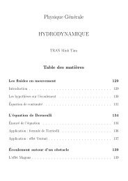
Figure 4.14 (left) gives an example of a mass plot for a particular experiment while figure
4.14 (right) shows , for 100 experiments, the deviation from truth of the fitted number of
signal events for each experiment.
35

N/20 GeV/c 2
16000
14000
12000
10000
8000
6000
4000
2000
0
0 40 80 120 160 200
Mass GeV/c 2
10
9
8
7
6
5
4
3
2
1
Mean
RMS
30.30
170.3
0
-800-600-400-200 0 200 400 600 800
Number of Events
Figure 4.14: Example of mass distribution obtained for one LHCb ”experiment” (left).
The backgrounds are represented in red in addition with the signal, which is in green at
the bottom. The black error bars represent the total number of generated events, with 1900
signal events generated. The plot on the right represents the distribution of the deviation
of the number of signal events reconstructed, from the number of signal events generated
(for 100 LHCb experiments).
The r.m.s of the deviation distributions for 100 experiments as a function of the average
number of events generated in each experiment is given in figure 4.15 (top). The most
interesting results is given by figure 4.15 (bottom) which shows that if the level of Higgs
production is the one predicted by the MSSM, a significance of 10σ could in principle be
reached after 1 LHCb running year 5 .
5 Here, once again, an enlarged acceptance has been used: 15 < θ < 390 mrad. Further studies will be
made with 15 < θ < 300 mrad.
36

N
N/ N
225
200
175
150
125
100
75
50
25
0
35
30
25
20
15
10
5
0
0 1000 2000 3000 4000 5000 6000
N of Events
0 1000 2000 3000 4000 5000 6000
N of Events
Figure 4.15: R.m.s. of the deviation of the number of reconstructed signal events from the
number of generated ones, as a function of the number N of signal events generated (top).
The significance N/σN corresponds to the r.m.s. σN of the deviation histograms (in black)
or to the error resulting from the fit (in red) (bottom) . The MSSM value for 1 running
year is the vertical red line.
37

Chapter 5
Conclusion
This work was dedicated to the study of the h 0 → aa → b ¯ bb ¯ b process at LHCb. Three
main sources of four b quarks backgrounds have also been included. The standalone computer
program Pythia was used to generate signal events while Alpgen was used for the
backgrounds generation.
First, we have discussed jet reconstructions based on the cone algorithm and we have
given a method to combine them into pairs. Then, a and Higgs candidates have been
reconstructed. Next, an event selection procedure has been presented to discriminate between
signal and background events. Finally, a TMC was used to test the ability to extract
signal events and it has been shown that, at the level of Higgs production predicted by
the MSSM, a significance of 10 σ could in principle be reached for 1 LHCb running year 1 .
This study has been made only at the quadrivector level. Therefore, the next step
would be to incorporate all detectors effects including the interactions with the magnetic
field in a full simulation. Situations were signal and background quarks are both present
inside the acceptance must also be investigated.
Basing ourselves on what was presented here, we can conclude that there seems to be
a possibility to detect the Higgs boson at LHCb and this opportunity must be further
investigated.
1 and with the enlarged acceptance defined before.
39

Appendix A
Alpgen parameters
Parameter and explanation Value
imode, 1 generates weighted events and writes to file for later unweighting 1
Label for the produced files bbcc
Grid: The generator will use a new grid 0
Number of events per iteration and number of warm-up iterations 100000000 2
Number of events generated after warm-up 1000000000
ihvy: choose the heavy flavour type, here c quark 4
ihvy2: same as before to insure b ¯ bc¯c production 4
ebeam: beam energy in the center of mass frame 7000.0
ih2: Select pp collisions 1
ndns: Parton density function, CTEQ5L * is used 5
njets: Number of light jets 0
etabmax: Pseudo rapidity η maximum of b quarks 4.5
etacmax: Pseudo rapidity η maximum of c quarks 4.5
drbmin: ∆R minimum between b quarks 0.1
drcmin: ∆R minimum between c quarks 0.1
ptbmin: Minimum transverse momentum of b quarks 10
ptcmin: Minimum transverse momentum of c quarks 10
Table A.1: Chosen parameters for the first generation phase in Alpgen. These are the
parameters for the b ¯ bc¯c component of the background leading to 539 ′ 679 events generated.
41

Parameter and explanation Value
imode, 1 generates weighted events and writes to file for later unweighting 1
Label for the produced files bbtt
Grid: The generator will use a new grid 0
Number of events per iteration and number of warm-up iterations 1000000 2
Number of events generated after warm-up 10000000
ihvy: choose the heavy flavour type, here t quark 6
ihvy2: same as before to insure b ¯ bt¯t production 6
ebeam: beam energy in the center of mass frame 7000.0
ih2: Select pp collisions 1
ndns: Parton density function, CTEQ5L * is used 5
njets: Number of light jets 0
etabmax: Pseudo rapidity η maximum of b quarks 4.5
drbmin: ∆R minimum between b quarks 0.1
ptbmin: Minimum transverse momentum of b quarks 10
Table A.2: Chosen parameters for the first generation phase in Alpgen. These are the
parameters for the b ¯ bt¯t component of the background leading to 117 ′ 676 events generated.
Example of input file used for phase one:
1 ! imode
bbbb ! label for files
0 ! start with: 0=new grid, 1=previous warmup grid, 2=previous generation grid
10000 2 ! Nevents/iteration, N(warm-up iterations)
100000 ! Nevents generated after warm-up
** The above 5 lines provide mandatory inputs for all processes
** (Comment lines are introduced by the three asterisks)
** The lines below modify existing defaults for the hard process under study
** For a complete list of accessible parameters and their values,
** input ’print 1’ (to display on the screen) or ’print 2’ to write to file
ihvy 5
ihvy2 5
ebeam 7000.0
ih2 1
ndns 5
njets 0
etabmax 4.5
drbmin 0.1
ptbmin 10
Phase two is simply initiated by:
2 ! imode
bbbb ! label for files
42

Appendix B
Other plots
Figure B.1: Transverse momentum of the a candidates from the signal (black) and b ¯ bc¯c
background (red).
43

a mass: method of the nearest b
dN/dm
dN/dm
0.07
0.06
0.05
0.04
0.03
0.02
0.01
signal
noise
0
0 5 10 15 20 25 30 35 40
2
Mass [GeV/c ]
2 2
a mass: minimisation of R +R
1 2
dN/dM
0.07
0.06
0.05
0.04
0.03
0.02
0.01
signal
noise
0
0 5 10 15 20 25 30 35 40
2
Mass [GeV/c ]
Both reconstructio: signal
dN/dM
0.07
0.06
0.05
0.04
0.03
0.02
0.01
Methode des b les plus proches
2 2
Minimisation de R +R
1 2
0
0 5 10 15 20 25 30 35 40
2
Mass [GeV/c ]
Both reconstructions: noise
0.035 Methode des b les plus proches
0.03
0.025
0.02
0.015
0.01
0.005
2 2
Minimisation de R +R
1 2
0
0 5 10 15 20 25 30 35 40
2
Mass [GeV/c ]
a mass: method of the nearest b (other a)
dN/dm
dN/dm
0.06
0.05
0.04
0.03
0.02
0.01
signal
noise
0
0 5 10 15 20 25 30 35 40
2
Mass [GeV/c ]
2 2
a Mass: minimisation of R +R2(other
a)
1
dN/dM
0.06
0.05
0.04
0.03
0.02
0.01
signal
noise
0
0 5 10 15 20 25 30 35 40
2
Mass [GeV/c ]
Both reconstructions: signal (other a)
dN/dM
0.06
0.05
0.04
0.03
0.02
0.01
Methode des b les plus proches
2 2
Minimisation de R +R
1 2
0
0 5 10 15 20 25 30 35 40
2
Mass [GeV/c ]
Both reconstructions: noise (other a)
0.025
0.02
0.015
0.01
0.005
Methode des b les plus proches
2 2
Minimisation de R +R
1 2
0
0 5 10 15 20 25 30 35 40
2
Mass [GeV/c ]
Figure B.2: Comparison between two different methods of jets combinations.
44

Bibliography
[1] DAVID E. KAPLAN and MATTHEW MCEVOY, Searching for Higgs decays to four
bottom quarks at LHCb, arXiv:hep-ph/09091521 v1, 8 September 2009
[2] LAURENT LOCATELLI, Direct Search for Higgs Boson in LHCb and Contribution
to the Development of the Vertex Detector, Thèse n°3868 (2007), Ecole Polytechnique
Fédérale de Lausanne
[3] NEAL GUEISSAZ, Searching for a Supersymmetric Higgs Boson through displaced
Decay Vertices in LHCb, Master Thesis (2007), Ecole Polytechnique Fédérale de Lausanne
[4] MICHELANGELO L. MANGANO, FLUVIO PICCININI and ANTONIO D.
POLOSA, ALPGEN, a generator for hard multiparton processes in hadronic collisions,
hep-ph/0206293 V2.1, December 2006
[5] AURELIO BAY and CEDRIC POTTERAT, A b jet ”seed” finder, LHCb-INT-2009-
023 V. 1, Laboratoire de Physique des Hautes Energies, EPFL, October 2009
[6] PIERRE JATON, Recherche d’une particule SuperSymétrique à LHCb avec violation
de la R-parité : le neutralino ˜χ 0 1 , Projet de Master, Laboratoire de Physique des
Hautes Energies, EPFL, automne 2008
[7] MICHAEL METCALF and JOHN REID, FORTRAN 90/95 explained, second edition,Oxford
University Press, 1999
[8] TORBJÖRN SJÖSTRAND, STEPHEN MRENNA and PETER SKANDS, PYTHIA
6.4 Physics and Manual, hep-ph/0603175, FERMILAB-PUB-06-052-CD-T, March
2006
[9] R. PITTAU, The Alpgen Generator, Granada, January/February 2008
[10] C. AMSLER et al., Particle Physics Booklet, extracted from the Review of Particle
Physics, Physics Letters B667, 1 (2008)
[11] M. E. PESKIN and D. V. SCHROEDER, An Introduction To Quantum Field Theory,
Westview Press, October 1995
45