Discovering and proving geometric inequalities by CAS (pdf)

Introduction
DISCOVERING AND PROVING
GEOMETRIC INEQUALITIES
Pavel Pech
University of South Bohemia, Czech Republic
email: pech@pf.jcu.cz
’Computer is like microscope which enables to observe new
worlds which are invisible with our eyes.‘
T. Recio, Univ. Santander
When a basic book Mechanical Geometry Theorem Proving written by Chinese mathematician
S. Ch. Chou appeared [2] in 1987, American mathematician Larry Woss wrote
in its preface:
’When computers were first conceived, the designed, and finally implemented, few people
(if any) would have conjectured that in 1987 computer programs would exist capable of
proving theorems from diverse areas of mathematics.
Even further, if a person at the inception of the computer age had seriously predicted that
computer programs would be used to occasionally answer open questions taken from mathematics,
that person would have received at best a polite smile.‘
Computer algebra methods based on results of commutative algebra like Groebner bases of
ideals and elimination of variables make it possible to solve complex, elementary and non
elementary problems of geometry, which are difficult to solve using a classical approach.
Computer algebra methods enable to prove geometric theorems, automatic derivation and
discovery of formulas, construction of objects which have given properties and which cannot
be easily done with a ruler and compass, etc. On the other hand classical methods
offer better insight into geometric situations, show the beauty of geometry and enable
better understanding the problem.
For the past few last semesters I have led at the University of South Bohemia a geometry
seminar on using computer methods to solve problems in elementary geometry. The
students involved were enrolled on a teacher training course in mathematics and were in
their 4th year of university study, i.e., they had knowledge of basic courses in geometry.
In the seminar methods based on Groebner bases computations were stressed. We used
these methods to prove and discover statements from geometry in a plane and a space.
1

We also used this theory to carry out constructions of geometric objects which have given
properties and which are not easy to construct by using ruler and compass.
Automatic theorem proving
Automatic theorem proving is concerned with geometry statements of equality type, which
are of the kind H ⇒ C, whereH is the set of hypotheses and C the conclusion.
First we express the geometric problem in an algebraic form. Let K be a field of characteristic
0, e.g. the field of rational numbers, and L be an algebraically closed which contains
K, e.g. the field of complex numbers. The first stage of automatic theorem proving is
characterized by establishing the set of hypotheses H whose algebraic form are polynomial
equations
h1(x1,x2,...,xn) =0, h2(x1,x2,...,xn) =0,...,hr(x1,x2,...,xn) =0
and the conclusion C, which is expressed by the polynomial equation
c(x1,x2,...,xn) =0,
where h1,h2,...,hr,c∈ K[x1,x2,...,xn]. Thus the algebraic form of the statement is
∀x ∈ L n , h1(x) =0, h2(x) =0, ..., hr(x) =0 ⇒ c(x) =0, (1)
where we write x instead x1,x2,...,xn. The objective of the next step is a verification
of (1). We are to decide whether the conclusion follows from the hypotheses or, which is
the same, to decide whether the zero set of the conclusion C contains the zero set of the
hypotheses H, i.e., Zero (H) ⊂ Zero (C).
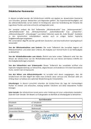
By the well-known Hilbert Nullstellensatz Theorem, the statement (1) is true iff 1 belongs
Figure 1: H ⇒ C ⇔ Zero(H) ⊂ Zero(C)
to the ideal (h1,h2,...,hr,ct − 1) of the hypotheses polynomials and negated conclusion.
However for most geometry problems it suffices to show that c belongs to the ideal
(h1,h2,...,hr). If yes we say that a statement (1) is generally true.
See a nice book [3] for further study.
Parallelogram law
To demonstrate the base of automatic theorem proving we start with investigation of
equalities between diagonals holding for various types of quadrilaterals. We will explore
the equality between the sum of squares of sides and the sum of squares of diagonals of a
parallelogram. This equality is known as the parallelogram law [6]:

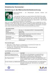
Given a parallelogram with the lengths of sides a, b and diagonals e, f. Then
Let us prove the relation (2) by computer.
2(a 2 + b 2 )=e 2 + f 2 . (2)
Denote the vertices of a parallelogram by letters A, B, C, D and its lengths of sides and
diagonals by a = |AB| = |CD|,b= |BC| = |DA|,e= |AC|,f = |BD|.
Choose the coordinate system such that A =[0, 0],B =[a, 0],C =[x, y],D =[x − a, y].
Then
b = |BC|⇔h1 :(x − a) 2 + y 2 = b 2 ,
e = |AC| ⇔h2 : x 2 + y 2 = e 2 ,
f = |BD|⇔h3 :(x − 2a) 2 + y 2 = f 2 .
The conclusion c is of the form
c :2(a 2 + b 2 )=e 2 + f 2 .
Figure 2: Parallelogram law: 2(a 2 + b 2 )=e 2 + f 2
We have an ideal I =(h1,h2,h3) and we are to show that the conclusion polynomial
c belongs to this ideal (or more exactly to the radical of I). We enter conditions into
CoCoA 1 and get
Use R::=Q[axybeft];
I:=Ideal((x-a)^2+y^2-b^2,x^2+y^2-e^2,(x-2a)^2+y^2-f^2);
NF(2(a^2+b^2)-(e^2+f^2),I);
the result 0 means that the polynomial c can be expressed as the linear combination of
hypotheses polynomials h1,h2,h3. Representation of c in terms of generators h1,h2,h3 can
be shown by the command GenRepr and is as follows
2(a 2 +b 2 )−(e 2 +f 2 )=−2·((x−a) 2 +y 2 −b 2 )+1·(x 2 +y 2 −e 2 )+1·((x−2a) 2 +y 2 −f 2 )).
The parallelogram law is proved.
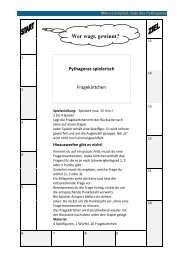
A classical proof of the equality (2) is as follows:
By the law of cosines in the triangle ABC it holds
Analogously in the triangle ABD we have
e 2 = a 2 + b 2 − 2ab cos ϕ.
f 2 = a 2 + b 2 − 2ab cos(π − ϕ).
1 Software CoCoA is distributed at cocoa@dima.unige.it

Figure 3: Parallelogram law: 2(a 2 + b 2 )=e 2 + f 2
Summing up both equalities we get (2).
We proved the statement above both in an automatic and classical way. Both methods
have their strengths and weaknesses. The classical way required basic knowledge from
elementary geometry (we used the law of cosines, etc.), gives us a good insight into the
problem, but had one weakness - we had to have the key idea how to prove the statement.
This is not always easy to find.
On the other hand the automatic proof required basic knowledge from analytical geometry
(”clever” introduction of coordinate system, expression of distances od vertices analytically,
etc.), the computation was quite automatic. But this method was not so beautiful
in geometric sense. This method can also lead to unexpected problems - e.g. to find non
- degeneracy conditions.
When students were asked which method they preferred and why, the answer was: ”the
classical method because of a better insight into the problem.” They agreed with the conclusion
that both methods should be combined and used in practice.
Remark:
The parallelogram law (2) had been already known in a little bit different form to ancient
Greeks. It became familiar since the year 1935, when Jordan and von Neumann showed
that Banach space in which (2) holds, is Hilbert space.
The parallelogram law (2) can be generalized on a trapezoid:
A quadrangle ABCD is a trapezoid with bases a, c, legs b, d and diagonals e, f if and only
if
b 2 + d 2 +2ac = e 2 + f 2 . (3)
We will leave the proof to the reader.
The relation
2(a 2 + b 2 )=e 2 + f 2 .
is a necessary condition for a quadrilateral ABCD to be a parallelogram. Is this condition
also a sufficient condition?
We will prove the following statement:
A quadrilateral ABCD with sides a, b, c, d and diagonals e, f is given. Then ABCD is a
parallelogram if and only if it holds
a 2 + b 2 + c 2 + d 2 = e 2 + f 2 . (4)

Figure 4: In a trapezoid b 2 + d 2 +2ac = e 2 + f 2 holds
One part of a statement has been already proved. Now assume that (4) is holding and we
will explore all quadrilaterals which fulfil (4). We will show that ABCD is a parallelogram.
Denote a = |AB|,b = |BC|,c = |CD|,d = |DA|,e = |AC|,f = |BD| and let A =
[0, 0],B =[a, 0],C =[x, y],D =[u, v]. Then |BC| = b ⇔ h1 :(x − a) 2 + y 2 = b 2 ,
Figure 5: a 2 + b 2 + c 2 + d 2 = e 2 + f 2 ⇔ ABCD is a parallelogram
|CD| = c ⇔ h2 :(x − u) 2 +(y − v) 2 = c 2 ,
|DA| = d ⇔ h3 : u 2 + v 2 = d 2 ,
|AC| = e ⇔ h4 : x 2 + y 2 = e 2 ,
|BD| = f ⇔ h5 :(u − a) 2 + v 2 = f 2 ,
h6 : a 2 + b 2 + c 2 + d 2 = e 2 + f 2 .
In the ideal I =(h1,h2,...,h6) we eliminate dependent variables b, c, d, e, f. We get
Use R::=Q[xyuvabcdef];
I:=Ideal((x-a)^2+y^2-b^2,(x-u)^2+(y-v)^2-c^2,u^2+v^2-d^2,x^2
+y^2-e^2,(u-a)^2+v^2-f^2,a^2+b^2+c^2+d^2-e^2-f^2);
Elim(b..f,I);
the only condition x 2 + y 2 − 2xu + u 2 − 2yv + v 2 − 2xa +2ua + a 2 = 0 which is equivalent
to
(x − u − a) 2 +(y − v) 2 =0. (5)
The condition (5) follows from given assumptions. It means that a quadrilateral is a
parallelogram since for real numbers x, y, u, v, a the condition (5) implies x − u − a =0

and y − v =0, i.e., that A − D = B − C.
Formal verification
Use R::=Q[xyuvabcdef];
I:=Ideal((x-a)^2+y^2-b^2,(x-u)^2+(y-v)^2-c^2,u^2+v^2-d^2,x^2
+y^2-e^2,(u-a)^2+v^2-f^2,a^2+b^2+c^2+d^2-e^2-f^2);
NF((x-u-a)^2+(y-v)^2,I);
confirms that normal form equals 0 and a quadrilateral which fulfils a 2 +b 2 +c 2 +d 2 = e 2 +f 2
is a parallelogram. The statement is true.
Remark:
If we would enter x − u − a =0andy − v =0, instead of the ”equivalent” condition
(x − u − a) 2 +(y − v) 2 =0, which also characterizes a parallelogram, we have failed. We
get
Use R ::= Q[xyuvabcdefts];
I:=Ideal((x-a)^2+y^2-b^2,(x-u)^2+(y-v)^2-c^2,u^2+v^2-d^2,
x^2+y^2-e^2,(u-a)^2+v^2-f^2,a^2+b^2+c^2+d^2-e^2-f^2,(x-u-a)t-1);
NF(1,I);
the result 1.
What is the difference between the conditions
(x − u − a) 2 +(y − v) 2 =0 and x − u − a =0∧ y − v =0?
’The only difference‘ consists in the fact that whereas in a real case both conditions are
the same, in the case of complex numbers is (x − u − a) 2 +(y − v) 2 =(x − u − a +
i(y − v))(x − u − a − i(y − v)), i.e., we get two conditions x − u − a + i(y − v) =0 ∨
x − u − a − i(y − v) =0!
This example should be instructive.
We have always to consider such conditions which the system requires (and mostly yields).
Any ”changes” of these conditions, despite they describe the reality properly, mostly lead
to the failure.
Solving inequalities
We will study some geometric inequalities discovered and proved by means of Buchberger’s
algorithm for computing Groebner bases of ideals. However we should realize that we are
working in an algebraic closed field, in our case in the field of complex numbers which, as
known, can not be ordered. Hence we can not use the signs > or

Inequality between diagonals of a quadrilateral
The following statement is a generalization of the parallelogram law on an arbitrary quadrilateral.
It holds:
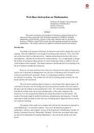
Given a quadrilateral ABCD with lengths of sides a, b, c, d and diagonals e, f. Then
a 2 + b 2 + c 2 + d 2 ≥ e 2 + f 2 . (6)
The sign of equality in (6) is attained if and only if ABCD is a parallelogram.
Let a = |AB|,b = |BC|,c = |CD|,d = |DA|,e = |AC|,f = |BD| and A =[0, 0],B =
[a, 0],C =[x, y],D =[u, v]. Then
Figure 6: In a quadrilateral ABCD the inequality a 2 + b 2 + c 2 + d 2 ≥ e 2 + f 2 holds
b = |BC|⇔h1 :(x− a) 2 + y2 = b2 ,
c = |CD|⇔h2 :(x− u) 2 +(y − v) 2 = c2 ,
d = |DA| ⇔h3 : u2 + v2 = d2 ,
e = |AC| ⇔h4 : x2 + y2 = e2 ,
f = |BD|⇔h5 :(u− a) 2 + v2 = f 2 .
To prove (6), we will try to express the difference (a2 + b2 + c2 + d2 ) − (e2 + f 2 )insuch
a form from which non - negativity of (a2 + b2 + c2 + d2 ) − (e2 + f 2 ) would follow. We
introduce a new variable k and put
hence let
h6 :(a 2 + b 2 + c 2 + d 2 ) − (e 2 + f 2 ) − k =0.
(a 2 + b 2 + c 2 + d 2 ) − (e 2 + f 2 )=k, (7)
In the ideal I =(h1,h2,...,h6) we eliminate dependent variables b, c, d, e, f to express k
in terms of independent variables x, y, u, v, a.
We get in CoCoA using the command Elim
Use R::=Q[xyuvabcdefk];
J:=Ideal((x-a)^2+y^2-b^2,(x-u)^2+(y-v)^2-c^2,u^2+v^2-d^2,
x^2+y^2-e^2,(u-a)^2+v^2-f^2,a^2+b^2+c^2+d^2-e^2-f^2-k);
Elim(b..f,J);
or in Derive using the command GROEBNER BASIS

2 2 2 2 2 2 2
GROEBNER_BASIS((x-a) + y - b ,(x-u) + (y-v) - c , u +
2 2 2 2 2 2 2 2 2 2 2 2 2
v - d , x + y - e ,(u-a) + v - f , a + b + c + d - e -
2
f - k, [b, c, d, e, f, a, x, y, u, v, k])
the polynomial
x 2 + y 2 − 2xu + u 2 − 2yv + v 2 − 2xa +2ua + a 2 − k.
This polynomial can be expressed in the form of the sum of squares
k =(x − u − a) 2 +(y − v) 2 . (8)
Substitution of k from (8) into (7) gives the following identity
a 2 + b 2 + c 2 + d 2 − e 2 − f 2 =(x − u − a) 2 +(y − v) 2 , (9)
which implies the inequality (6). The equality in (6) is attained if and only if ABCD is a
parallelogram as we could see from the parallelogram law.
Instead of (6) we can write (9) which describes the situation better including the case of
equality. By (9) we rediscovered the theorem which is ascribed to L. Euler [8]:
Given a skew quadrilateral ABCD. DenoteP, Q the midpoints of diagonals AC and BD
respectively. Then
|AB| 2 + |BC| 2 + |CD| 2 + |DA| 2 −|AC| 2 −|BD| 2 =4|PQ| 2 . (10)
A close inspection shows that the relation (10) is equal to (9).
Figure 7: In a skew quadrilateral |AB| 2 +|BC| 2 +|CD| 2 +|DA| 2 = |AC| 2 +|BD| 2 +4|PQ| 2
holds
General case
The inequality (6) is a special case of the following theorem which was published in 1980
by L. Gerber [6]:
Let Π=P0,P1,...,Pn−1 be a closed skew n-gon in the Euclidean space E N . Then
n−1
k=0
|PkPk+2| 2 n−1
2 π
≤ 4cos
n
k=0
|PkPk+1| 2 , (11)

with the equality if and only if Π is a planar affine-regular n-gon.
For n = 4 we get the relation (6) since an affine image of a square is a parallelogram.
Another generalization of the inequality (11) was published in 1990 by P. Pech, see [11].
It is as follows:
Let Π=P0,P1,...,Pn−1 be a closed skew n-gon in the Euclidean space E N and let Pn+j =
Pj, for j =0, 1,... Then for all p =0, 1,...,n− 1
n−1
2 π
sin |PkPk+p|
n
k=0
2 ≤ sin 2 (p π
n )
n−1
k=0
with the equality if and only if Π is a planar affine-regular n-gon.
For p = 2 we get from (12) the inequality (11).
Euler’s inequality
|PkPk+1| 2 , (12)
In 1765 L. Euler [5] published the relation (13) which expresses the distance d of the
incenter and circumcenter of an arbitrary triangle
where r is the circumradius and p is the inradius.
d = r(r − 2p) , (13)
In [10] it is given that H. Wieleitner [14] mentions, that the relation (13) was published
Figure 8: Euler’s relation: d = r(r − 2p)
even earlier by W. Chapple from England in 1746.
The following inequality, which is a consequence of (13), is
r ≥ 2p , (14)
called Euler’s inequality [4]. It is obvious that the equality in (14) is attained iff a triangle
is equilateral, because only in this case the circumcenter and incenter coincide and d =0
in (13).
We will prove the Euler’s inequality (14) by computer. We will proceed in a similar way
as W. Koepf [7] without introducing a coordinate system.
Let ABC be an arbitrary triangle with the lengths of sides a, b, c. Denote by r and p its

circumradius and inradius respectively and let f be the area of ABC. For the area f of a
triangle ABC we have the following familiar relations:
h1 : f − p(a + b + c)/2 =0,
h2 : f − abc/(4r) =0,
h3 :16f 2 − (a + b + c)(−a + b + c)(a − b + c)(a + b − c) =0.
Suppose that a, b, c, p, r, f are positive real numbers. The main idea of the method is as
follows. We will try to express r − 2p in such a form from which it would be clear that
r − 2p is greater than or equals zero. That is why we introduce a slack variable k such
that r − 2p = k, i.e.,
h4 : r − 2p − k.
In the ideal I =(h1,h2,h3,h4) we will eliminate p and r to obtain polynomials in variables
a, b, c, f, k. We enter in CoCoA using the command Elim
Use R::=Q[abcprfk];
I:=Ideal(2f-p(a+b+c),4fr-abc,16f^2-(a+b+c)(-a+b+c)(a-b+c)(a+b-c),
r-2p-k);
Elim(p..r,I);
and get a few polynomials from which the following one, after dividing it with a non zero
factor f, leads to the equation of the form
4fk = a 3 − a 2 b − ab 2 + b 3 − a 2 c +3abc − b 2 c − ac 2 − bc 2 + c 3 . (15)
From (15) we see that the expression k = r − 2p is non-negative iff the polynomial on the
right in (15) is non-negative. It is easy to show that the equality
a 3 − a 2 b − ab 2 + b 3 − a 2 c +3abc − b 2 c − ac 2 − bc 2 + c 3 =
=1/2[(a + b − c)(a − b) 2 +(b + c − a)(b − c) 2 +(c + a − b)(c − a) 2 ] (16)
holds, cf. [7]. The expression on the right hand side in (16) is non-negative. Namely it is
the sum of non negative expressions which consist of squares (a − b) 2 , (b − c) 2 , (c − a) 2 and
expressions a + b − c, b + c − a, c + a − b which are positive due to the triangle inequality.
The equality in (14) occurs if and only if a = b = c in (16) on the right, i.e., iff a triangle
ABC is equilateral.
Remark:
In order to prove (14) we could also prove the equality (13) from which the inequality (14)
follows, see [13].
The following classical proof is ascribed to Hungarian mathematician I. Ádám [10]. His
proof is very smart:
The midpoints A1,B1,C1 of sides of a triangle ABC form a triangle whose circumcircle
has the radius r/2. Construct a triangle A ′ B ′ C ′ whose sides are parallel to the sides of a
triangle ABC so that the circumcircle of a triangle A1,B1,C1 is the incircle of A ′ B ′ C ′ .
Since △ABC ⊆△A ′ B ′ C ′ then for inradii p, r/2 of both triangles the relation p ≤ r/2
holds. The classical proof is now complete.
The proof just given can be easily applied to a tetrahedron and in general to an arbitrary
simplex in n-dimensional Euclidean space E n . For the radii p and r of spheres which are
inscribed and circumscribed to a tetrahedron analogous relation to (14)
r ≥ 3p , (17)
holds. The midpoints of sides are then replaced by the centroids of faces of a tetrahedron.

References
Figure 9: A classical proof of the Euler’s inequality
[1] W. Blaschke: Kreis und Kugel. Walter de Gruyter & Co, Berlin 1956.
[2] S.C. Chou: Mechanical Geometry Theorem Proving. D. Reidel Publishing Company,
Dordrecht 1987.
[3] D. Cox, J. Little, D. O’Shea: Ideals, Varieties, and Algorithms. Second Edition,
Springer 1997.
[4] O. Bottema et al: Geometric inequalities. Groningen 1969.
[5] L. Euleri: Novi commentarii academicae scientiarum Petropolitanae 11 (1765),
1767, 103-123.
[6] L. Gerber: Napoleon’s theorem and the parallelogram inequality for affine-regular
polygons. Amer. Math. Monthly 87 (1980), 644-648.
[7] W. Koepf: Gröbner Bases and Triangles. International Journal of Computer Algebra
in Mathematics Education 4 (1997), 371-386.
[8] A.G. Konforovič: V´yznamné matematické úlohy. SPN, Praha 1989.
[9] D.S. Mitrinovič, J.E. Pečarič, V. Volenec: Recent Advances in Geometric
Inequalities. Kluwer Academic Publishers, Dordrecht/Boston/London, 1989.
[10] Z. Nádeník: Náměty k stˇredoˇskolské geometrii. Pokroky matematiky, fyziky a astronomie
19, No. 6, (1974).
[11] P. Pech: Inequality between sides and diagonals of a space n-gon and its integral
analog. Čas. pro pěst. mat. 115 (1990), 343-350.
[12] P. Pech: Klasické versus počítačové metody pˇri ˇreˇsení problém˚u v geometrii .
Jihočeská univerzita v Česk´ych Budějovicích, 2005.
[13] D. Wang: Elimination Practice. Software Tools and Applications. Imperial College
Press, London, 2004.
[14] H. Wieleitner: Geschichte der Mathematik, II. Teil.1911-1921, Russian translation
1958, 2. edition 1966.