Hilbert-Huang transf..
Hilbert-Huang transf..
Hilbert-Huang transf..

Create successful ePaper yourself
Turn your PDF publications into a flip-book with our unique Google optimized e-Paper software.
Flow Measurement and Instrumentation 18 (2007) 37–46<br />
Flow Measurement<br />
and Instrumentation<br />
www.elsevier.com/locate/flowmeasinst<br />
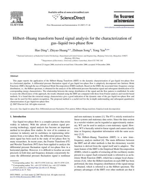
<strong>Hilbert</strong>–<strong>Huang</strong> <strong>transf</strong>orm based signal analysis for the characterization of<br />
gas–liquid two-phase flow<br />
Abstract<br />
Hao Ding a , Zhiyao <strong>Huang</strong> a,∗ , Zhihuan Song a , Yong Yan b,∗∗<br />
a National Laboratory of Industrial Control Technology, Department of Control Science and Engineering, Zhejiang University, Hangzhou 310027,<br />
Zhejiang, PR China<br />
b Department of Electronics, University of Kent, Canterbury, Kent CT2 7NT, UK<br />
Received 25 August 2006; received in revised form 3 December 2006; accepted 19 December 2006<br />
This paper reports the application of the <strong>Hilbert</strong>–<strong>Huang</strong> Transform (HHT) to the dynamic characterization of gas–liquid two-phase flow<br />
in a horizontal pipeline. A differential pressure fluctuation signal of gas–liquid two-phase flow is adaptively decomposed into Intrinsic Mode<br />
Functions (IMFs) through the use of Empirical Mode Decomposition (EMD) methods. Based on the EMD, the associated time–frequency–energy<br />
distribution, i.e., the <strong>Hilbert</strong> spectrum, is obtained for the analysis of the differential pressure fluctuation signal and subsequent identification of its<br />
corresponding energy characteristics. The relationship between the energy distribution of the signal and the flow pattern is established. In order<br />
to assess the effectiveness of the approach, the results obtained using the HHT are compared with those from Fourier analysis and wavelet based<br />
methods. It is found that the extracted energy characteristics give a good indication of the dynamic state of the gas–liquid two-phase flow and<br />
thus can be used for flow pattern recognition. The proposed method is a useful tool for the in-depth understanding and subsequent quantitative<br />
characterization of gas–liquid two-phase flow.<br />
c○ 2007 Elsevier Ltd. All rights reserved.<br />
Keywords: Gas–liquid two-phase flow; Differential pressure fluctuation; Flow pattern; <strong>Hilbert</strong>–<strong>Huang</strong> <strong>transf</strong>orm; Empirical mode decomposition<br />
1. Introduction<br />
Gas–liquid two-phase flow is a complex process that exists<br />
widely in industry. With the advent of modern signal processing<br />
technology, signal analysis has become an important<br />
method in two-phase flow studies. In view of its common occurrence<br />
in industry and its usefulness in representing information<br />
from a two-phase flow, the differential pressure fluctuation<br />
signal has been used in the study of two-phase flow by<br />
many researchers. In recent years, the Fourier Transform (FT)<br />
and Wavelet Transform (WT) have been applied to analyze the<br />
differential pressure fluctuation signal of two-phase flow in a<br />
horizontal pipeline. However, it is difficult to localize an event<br />
precisely in both time and frequency domains concurrently because<br />
the differential pressure fluctuation signal is nonlinear<br />
∗ Corresponding author. Tel.: +86 571 8795 2145; fax: +86 571 8795 1219.<br />
∗∗ Corresponding author. Tel.: +44 1227 823015; fax: +44 1227 456084.<br />
E-mail addresses: zyhuang@iipc.zju.edu.cn (Z. <strong>Huang</strong>),<br />
y.yan@kent.ac.uk (Y. Yan).<br />
0955-5986/$ - see front matter c○ 2007 Elsevier Ltd. All rights reserved.<br />
doi:10.1016/j.flowmeasinst.2006.12.004<br />
and non-stationary in nature [1]. The FT is strictly restricted to<br />
linear systems and stationary data series. Since the data section<br />
in a wavelet window can be regarded as approximately stationary,<br />
WT can be used to analyze a non-stationary signal. However,<br />
WT is basically suited to linear signals and cannot classify<br />
time or frequency dependent information with the same accuracy<br />
[2,3].<br />
The <strong>Hilbert</strong>–<strong>Huang</strong> Transform (HHT) is a new time–<br />
frequency analysis method [4]. The main difference between<br />
the HHT and all other methods is that the elementary wavelet<br />
function is derived from the signal itself and is adaptive. The<br />
main feature of the HHT is the Empirical Mode Decomposition<br />
(EMD), which is capable of extracting all the oscillatory modes<br />
present in a signal. Each extracted mode is referred to as an Intrinsic<br />
Mode Function (IMF), which has a unique local characteristic<br />
[5,6]. After the <strong>Hilbert</strong> <strong>transf</strong>orm on each IMF has been<br />
performed, the time–frequency distribution of the signal energy<br />
is obtained, which is referred to as the <strong>Hilbert</strong> spectrum. The<br />
primary advantages of the HHT over other methods are that it
38 H. Ding et al. / Flow Measurement and Instrumentation 18 (2007) 37–46<br />
can deal with the nonlinear problem objectively and the resolutions<br />
of the <strong>Hilbert</strong> spectrum are satisfactory in both time and<br />
frequency domains. The HHT is therefore suited to the exploration<br />
of the local properties of a signal [7].<br />
The HHT has been widely applied in recent years in the<br />
fields of meteorology, ocean engineering, earthquake studies,<br />
etc. Useful research results have been achieved to date, but<br />
very limited work has been reported on the method for the<br />
monitoring and characterization of two-phase flow. This paper<br />
describes how the HHT is applied to analyze a differential<br />
pressure fluctuation signal for the dynamic characterization<br />
of gas–liquid two-phase flow. The local characteristics of<br />
the signal are extracted and quantified under typical flow<br />
conditions. A direct comparison between the HHT and FT<br />
methods is also presented.<br />
2. Fourier <strong>transf</strong>orm versus wavelet <strong>transf</strong>orm<br />
The conventional FT uses linear superposition of trigonometric<br />
functions to approach the original signal [4]. The FT of<br />
the signal f (t) ∈ L2 (R) is defined as<br />
F(ω) =<br />
∞<br />
−∞<br />
f (t)e − jωt dt (1)<br />
where ω is the angular frequency.<br />
Although the FT is valid under general conditions, there<br />
are some critical restrictions. As the FT is used to analyze a<br />
signal, many additional components are introduced, giving rise<br />
to misleading results. In order to overcome this shortcoming,<br />
windowed FT is proposed, in which a time–frequency<br />
distribution is obtained by sliding the window along the time<br />
axis. Since this method depends on the conventional FT, the<br />
analysis data are assumed to be piecewise-stationary. However,<br />
there are practical difficulties in applying the method: in<br />
order to localize an event in the time domain, the window<br />
width must be narrow enough; on the other hand, the<br />
frequency resolution requires longer time series [2]. These<br />
contradictory requirements have posed significant limitations<br />
on the applicability of the FT.<br />
Unlike the FT, WT is a time–frequency analysis tool suitable<br />
for non-stationary signal analysis. WT can be interpreted as a<br />
decomposition of a signal into a set of frequency bands with the<br />
same bandwidth on a logarithmic scale. The elementary wavelet<br />
function is expressed as<br />
ψa,b(t) = |a| − 1 <br />
t − b<br />
2 ψ<br />
a, b ∈ R a = 0 (2)<br />
a<br />
where a is the dilation factor and b is the translation factor. On<br />
the other hand, 1/a denotes the frequency scale and b defines<br />
the location of an event. The corresponding continuous WT can<br />
be defined by<br />
W f (a, b) = 〈 f, ψa,b〉 = |a| − 1 <br />
t − b<br />
2 f (t)ψ dt (3)<br />
a<br />
where f (t) represents the signal to be analyzed.<br />
WT can be viewed as an extended version of Fourier analysis<br />
but with an adjustable window using short windows at high<br />
R<br />
frequency and long windows at low frequency [2,3]. Since<br />
WT is fundamentally still based on Fourier analysis, all the<br />
possible complications associated with the FT still exist. WT<br />
satisfies the Heisenberg inequality, thus the resolutions in the<br />
time and frequency domains cannot have the same accuracy<br />
simultaneously. For practical applications, the elementary<br />
wavelet function, ψ(·), can be adaptively modified by changing<br />
the dilation factor and the translation factor. However, the<br />
elementary wavelet function has to be given beforehand and<br />
is difficult to change during analysis. The main drawback of<br />
WT is that the fixed elementary wavelet function does not<br />
necessarily match the varying nature of a signal. In practice,<br />
it is difficult for WT to obtain a quantitative definition of the<br />
energy–frequency–time distribution by the limited size of the<br />
elementary wavelet function [4,8].<br />
3. <strong>Hilbert</strong>–<strong>Huang</strong> <strong>transf</strong>orm<br />
The HHT process comprises two main steps. Firstly, IMFs<br />
are extracted from the signal itself based on EMD. Secondly,<br />
the <strong>Hilbert</strong> <strong>transf</strong>orm is applied to each IMF component.<br />
Consequently, the instantaneous frequency can be calculated<br />
and the energy distribution of the signal is obtained in the<br />
time–frequency plane [9–11].<br />
3.1. EMD method<br />
EMD is an adaptive technique that decomposes the original<br />
signal into a family of IMF components. Each component<br />
emphasizes the local embedded characteristics of the signal. An<br />
IMF must satisfy two constraints: (i) the number of extrema and<br />
the number of zero crossings must either equal each other or<br />
differ at most by one; and (ii) at any time, the mean value of the<br />
envelope defined by the local maxima and the envelope defined<br />
by the local minima is zero.<br />
The first constraint is similar to the traditional narrow-band<br />
requirements for a stationary Gaussian process. The second<br />
constraint modifies the global requirement to a local one and is<br />
necessary so that the instantaneous frequency will not include<br />
unwanted fluctuations.<br />
The decomposition of data series x(t) follows a number of<br />
logical steps [12,13]. These are described below.<br />
1. Identify all of the local maxima and local minima of the<br />
signal x(t). Then use cubic spline interpolation to define the<br />
upper envelope xmax(t) and the lower envelope xmin(t) of the<br />
original data series. The mean m1(t) of the upper and lower<br />
envelopes is calculated as follows:<br />
m1(t) = xmax(t) + xmin(t)<br />
. (4)<br />
2<br />
2. Subtracting m1(t) from the data series x(t) gives:<br />
h1(t) = x(t) − m1(t). (5)<br />
3. In general, h1(t) is just an IMF candidate that is unlikely<br />
to satisfy all the requirements of IMF. Iterate the above<br />
procedure k times until the mean envelope is close to zero,
so the first IMF component I1(t) that contains the highest<br />
frequency component of the signal can be designated as<br />
h1(k−1)(t) − m1k(t) = h1k(t), I1(t) = h1k(t). (6)<br />
The above procedure is a sifting process that has two effects:<br />
(i) to eliminate riding waves; and (ii) to smooth uneven<br />
amplitude. In order to avoid obliterating the physically<br />
meaningful amplitude fluctuations, a stop criterion for the<br />
sifting process is defined [10].<br />
4. Separate I1(t) from the rest of the data series. The residue,<br />
r1(t), is treated as the new data series. Since the residue<br />
r1(t) still contains much information from lower frequency<br />
components, it is subjected to the same sifting process.<br />
Repeat the above procedure on the subsequent residual r j(t)<br />
until the range of the residue is below a predetermined value<br />
or the residue contains the lowest frequency component, and<br />
the result is<br />
r1(t) − I2(t) = r2(t), . . . , rn−1(t) − In(t) = rn(t) (7)<br />
where rn(t) denotes the trend of the signal from which no<br />
more IMF can be extracted and In is the nth IMF. Each IMF<br />
contains lower frequency components than the one extracted<br />
just before. At the end of the EMD procedure, the signal x(t)<br />
can be exactly reconstructed using a linear combination:<br />
n<br />
x(t) = Ii(t) + rn(t). (8)<br />
i=1<br />
3.2. <strong>Hilbert</strong> spectrum<br />
The <strong>Hilbert</strong> <strong>transf</strong>orm is applied to every IMF component<br />
Ii(t) to obtain a data series Li(t):<br />
Li(t) = 1<br />
π P<br />
∞<br />
−∞<br />
H. Ding et al. / Flow Measurement and Instrumentation 18 (2007) 37–46 39<br />
Ii(τ)<br />
dτ (9)<br />
t − τ<br />
where P is Cauchy principal value. An analytical signal Zi(t)<br />
can be constructed by<br />
Zi(t) = Ii(t) + j Li(t) = ai(t)e jθ j (t)<br />
(10)<br />
where the amplitude ai(t) and the phase θi(t) are determined<br />
from<br />
ai(t) = [Ii(t) + Li(t)] 1 2 , θi(t) = arctan Li(t)<br />
. (11)<br />
Ii(t)<br />
The instantaneous frequency ωi(t) of the analytical signal is<br />
defined as the first derivative of the phase θi(t) [14–16]:<br />
ωi(t) = 1<br />
2π<br />
dθi(t)<br />
. (12)<br />
dt<br />
¿From Eqs. (11) and (12), the instantaneous frequency<br />
and amplitude (energy) are all functions of time. The<br />
time–frequency distribution of the amplitude is referred to as<br />
the <strong>Hilbert</strong> spectrum:<br />
H(ω, t) = Re<br />
n<br />
ai(t)e<br />
i=1<br />
j ωi (t)dt<br />
where n is the number of IMFs.<br />
(13)<br />
Fig. 1. Experimental system: (1) water tank, (2) water pump, (3) water storage,<br />
(4) water flowmeter, (5) compressor, (6) air storage, (7) gas flowmeter, (8)<br />
mixer, (9) differential pressure transducer, (10) A/D converter, (11) computer.<br />
Then the marginal spectrum can be defined as<br />
h(ω) =<br />
T<br />
0<br />
H(ω, t)dt (14)<br />
where T is the total data length. The contribution of the total<br />
amplitude from each frequency is measured by the marginal<br />
spectrum.<br />
4. Experimental test rig<br />
The experimental set-up used in this study is shown in Fig. 1.<br />
The differential pressure transducer used was a PD-23 type<br />
differential pressure sensor. Fig. 1 indicates that two pressure<br />
probes were installed on each pipe. A long transparent section<br />
was installed upstream of the transducer so that the flow pattern<br />
could be observed. The internal diameters of the three pipelines<br />
at the test section are 15 mm, 25 mm and 40 mm, respectively.<br />
The spacing between the two pressure probes is 0.25 m. The<br />
gas flowrate mg was varied in the range of 0–10 m 3 /h and<br />
the water flowrate mw in the range of 0–3.5 m 3 /h. In each<br />
pipeline, the water flowrate was set to a constant value and<br />
the gas flowrate was increased gradually. With the change in<br />
gas flowrate, various flow patterns were created. A series of<br />
experiments was conducted for different flow patterns such as<br />
bubble flow, plug flow, wavy flow and slug flow. Through the<br />
A/D converter, the differential pressure fluctuation signal was<br />
fed into the computer for processing. The sampling frequency<br />
and the sampling duration were 200 Hz and 15 s, respectively.<br />
5. Results and discussion<br />
5.1. Energy characteristics extracted<br />
Fig. 2 shows side by side the IMF components and the<br />
wavelet components of the differential pressure fluctuation<br />
signal from the 25 mm-diameter pipeline.<br />
It can be seen from Fig. 2 that the IMFs have different<br />
local frequencies. The EMD method picks out the highestfrequency<br />
component present in the signal. Thus, each IMF<br />
component that contains a lower frequency than the preceding<br />
one extracted is presented in turn. Furthermore, the quantitative<br />
time–frequency representation is also obtained. EMD is a full<br />
data driven method. However, WT disintegrates the signal into
40 H. Ding et al. / Flow Measurement and Instrumentation 18 (2007) 37–46<br />
Fig. 2. Comparison between the IMF components and wavelet components of the differential pressure fluctuation signals from the 25 mm-diameter pipeline: (a)–(d)<br />
the IMF components; (e)–(h) the wavelet components.<br />
a series of scales that cannot reveal precisely the relationship<br />
between time and instantaneous frequency [4]. The smaller<br />
scales represent the high-frequency information in the signal<br />
and the larger scales represent the low-frequency information<br />
in the signal.<br />
In this study, the energy distribution H j of different<br />
frequency bands is defined as<br />
H j = E j<br />
E<br />
( j = 1, 2, 3) (15)
Table 1<br />
Distribution of energy characteristics H j of a 15 mm-diameter pipeline<br />
mg (m 3 /h) Flow pattern Energy characteristics H j (%)<br />
H1 H2 H3<br />
0.3 Bubble flow 87.69 10.17 2.14<br />
1.0 Plug flow 33.23 62.29 4.48<br />
1.5 Wavy flow 35.49 31.16 33.35<br />
2.0 Slug flow 10.60 22.88 66.52<br />
where E j stands for the local energy of the different frequency<br />
bands ( j = 1 denotes the high-frequency band, j = 2 the<br />
middle-frequency band and j = 3 the low-frequency band) and<br />
E is the total energy. The energy distribution H j is selected as<br />
the characteristics of the differential pressure fluctuation signal.<br />
In this study a number of logical steps were followed:<br />
(1) acquire the differential pressure fluctuation signal;<br />
(2) apply HHT to the signal;<br />
(3) compare the analysis results between HHT and WT;<br />
(4) calculate the total signal energy, each frequency band of<br />
local energy and the energy distribution;<br />
(5) determine the energy distribution of the signal.<br />
As per the extensive experimental work undertaken and<br />
literature published, the IMF components are divided into three<br />
frequency bands in terms of their inherent frequencies for<br />
quantitative analysis of the energy distribution: high-frequency<br />
band H1 (>25 Hz) with IMF components of I1 and I2, middlefrequency<br />
band H2 (5–25 Hz) with IMF components of I3,<br />
I4 and I5 and low-frequency band H3 (
42 H. Ding et al. / Flow Measurement and Instrumentation 18 (2007) 37–46<br />
Fig. 3. Comparison between <strong>Hilbert</strong> spectra and wavelet spectra of the differential pressure fluctuation signals for the 15 mm-diameter pipeline: (a)–(d) <strong>Hilbert</strong><br />
spectra; (e)–(h) wavelet spectra. (For interpretation of the references to colour in this figure legend, the reader is referred to the web version of this article.)<br />
The above results imply that the energy characteristic H j<br />
changes with the flow pattern and can therefore be regarded<br />
as an indicator for the identification of the flow pattern of<br />
gas–liquid two-phase flow. The results also demonstrate that<br />
the HHT is suitable for analyzing the differential pressure<br />
fluctuation signal. Moreover, the influence of the pipe diameter<br />
on the energy characteristic is not significant. Thus, the<br />
extracted energy characteristics can be used as an objective<br />
indicator for flow pattern monitoring of gas–liquid twophase<br />
flow. Though WT method can also be used to study<br />
gas–liquid two-phase flow, it is difficult to demonstrate the<br />
local characteristics of the signal in both time and frequency
domains because of the non-adaptive feature of the form of<br />
elementary wavelet function in a practical application [4]. In<br />
the next section, detailed analysis results for both HHT and WT<br />
will be given.<br />
5.2. Comparison between the HHT and WT methods<br />
The experimental results presented above indicate that the<br />
differential pressure fluctuation signals from different sized<br />
pipelines have similar spectral characteristics. So we take the<br />
experimental results for the 15 mm-diameter pipeline as an<br />
example to analyze the <strong>Hilbert</strong> spectrum and the WT spectrum<br />
of the signal. The <strong>Hilbert</strong> spectra and wavelet spectra of the<br />
typical flow patterns in the 15 mm-diameter pipeline are plotted<br />
in Fig. 3. The <strong>Hilbert</strong> spectra as the greyscale coded maps are<br />
shown on the left, while the wavelet spectra of the signals are<br />
illustrated on the right. The colour bars beside each <strong>Hilbert</strong><br />
spectrum denote the time and frequency dependent energy. The<br />
energy is normalized and represented on a logarithmic scale.<br />
The colour bars next to each wavelet spectrum represent the<br />
absolute wavelet coefficient, i.e., the amplitude of the signal [3].<br />
Fig. 3(a) shows the <strong>Hilbert</strong> spectrum of bubble flow. The<br />
fluctuations of differential pressure are stable and the amplitude<br />
of the signals is small. The main fluctuation locates at the higher<br />
frequency, consequently the energy concentrates mainly on the<br />
high-frequency components and the total energy is low. The<br />
energy is evenly distributed in the high-frequency plane over<br />
25 Hz in Fig. 3(a) and there is very little energy below 25 Hz.<br />
The wavelet spectrum shows a similar energy distribution as the<br />
<strong>Hilbert</strong> spectrum, as shown in Fig. 3(e). It can be seen that the<br />
energy concentrates mostly in the smaller scale range.<br />
Fig. 3(b) shows the <strong>Hilbert</strong> spectrum of the plug flow.<br />
Compared to the bubble flow, the ratio of energy embedded<br />
in different frequency bands is changed. The ratio of energy<br />
embedded in the high-frequency range has reduced rapidly<br />
whereas the ratio of energy embedded in the middle–lowfrequency<br />
range has increased. As there still exist many tiny<br />
bubbles between two successive plugs, there is low energy in<br />
H. Ding et al. / Flow Measurement and Instrumentation 18 (2007) 37–46 43<br />
Fig. 3. (continued)<br />
the high-frequency range. Fig. 3(f) shows the results derived<br />
from WT. It is clear that the peak amplitude is greater than that<br />
of the bubble flow.<br />
The <strong>Hilbert</strong> spectrum of the wavy flow (Fig. 3(c)) indicates<br />
that the ratio of energy embedded in the higher-frequency range<br />
is greater than that in other frequency ranges. Compared to<br />
the plug flow, the ratio of energy embedded in the middlefrequency<br />
range begins to decrease and that in the lowerfrequency<br />
range begins to increase slowly. As shown in<br />
Fig. 3(g), the ratio of energy embedded in smaller scales begins<br />
increasing.<br />
Fig. 3(d) depicts the <strong>Hilbert</strong> spectrum of the slug flow. The<br />
size of gas slug is bigger than the bubble and the fluctuation of<br />
the signal is more drastic than other three flow patterns. As a result,<br />
the ratio of energy embedded in the lower-frequency range<br />
is the greatest, which is consistent with the analysis result from<br />
the wavelet spectrum shown in Fig. 3(h). As shown in Fig. 3, the<br />
variation in the ratio of energy embedded in different frequency<br />
bands is distinctive in the <strong>Hilbert</strong> spectrum and is in agreement<br />
with the wavelet spectrum. However, the frequency and time<br />
localization of the <strong>Hilbert</strong> spectrum is superior to that of the<br />
wavelet spectrum. The localizations of WT are accomplished<br />
by modifying the scale of the elementary wavelet function. If a<br />
local event occurs in the low-frequency range, it is necessary to<br />
modify the scale for characterizing the signal continuously [4].<br />
WT indeed improves the time resolution as compared to the FT,<br />
but HHT gives much finer local properties than WT.<br />
Although Fig. 3 gives a comparison between the <strong>Hilbert</strong> and<br />
the wavelet spectra for the same set of data, the differences<br />
between the two methods are not so obvious according<br />
to the counter-intuitive figures. From a theoretical point of<br />
view, the choice of the elementary wavelet function will<br />
have a significant impact on the analysis results because the<br />
elementary wavelet function is fixed during analysis. Once<br />
the elementary function is determined, it will be used to<br />
analyze all the data [2,4]. Since WT is Fourier based, the<br />
wavelet spectrum possesses some fundamental characteristics<br />
of a Fourier spectrum. WT can analyze a non-stationary signal
44 H. Ding et al. / Flow Measurement and Instrumentation 18 (2007) 37–46<br />
Fig. 4. Comparison between marginal spectra and Fourier spectra of the differential pressure fluctuation signals for the 40 mm-diameter pipeline: (a)–(d) the<br />
marginal spectra; (e)–(h) the Fourier spectra.<br />
under the assumption that the signal inside each sliding window<br />
is stationary [17]. However, HHT is an efficient and adaptive<br />
method which requires no assumption about signal stationarity.<br />
HHT is capable of analyzing a nonlinear and non-stationary<br />
signal not limited by the Heisenberg inequality. A more precise<br />
time–frequency–energy representation may be obtained by<br />
using an adaptive basis to preserve intrinsic properties of a<br />
signal [8].<br />
The marginal spectrum provides a measure of total<br />
amplitude (or energy) contribution from each frequency value.<br />
It presents the cumulative amplitude over the entire data span.<br />
The Fourier spectrum depicts the global frequency–energy<br />
distribution [2]. Because the pipe diameter is not very<br />
significant for the signal analysis, only the experimental results<br />
for the 40 mm-diameter pipeline are presented here. The<br />
same variation trends exist for 15 mm- and 25 mm-diameter
pipelines. The marginal spectra and Fourier spectra are plotted<br />
in Fig. 4.<br />
It is evident from Fig. 4(a)–(d) that the ratio of energy<br />
embedded in different frequency bands varies with the change<br />
in flow pattern. Meanwhile, the energy amplitude of the signal<br />
increases with the variation of flow pattern. These results are<br />
in agreement with those of <strong>Hilbert</strong> spectra. Because stationarity<br />
and linearity are the crucial restrictions of the FT, the adoption<br />
of the stationary and linear assumptions may give misleading<br />
results [2]. When the FT is used to analyze the differential<br />
pressure fluctuation signal, many frequency components are<br />
introduced to simulate the inherent features of the signal, but<br />
their existence disperses the energy to a much wider frequency<br />
range [4]. Thus, these additional frequency components and<br />
the wide frequency spectra cannot accurately represent the true<br />
frequency–energy distribution.<br />
6. Conclusions<br />
The HHT has been applied in the analysis of a differential<br />
pressure fluctuation signal derived from gas–liquid two-phase<br />
flow in a horizontal pipeline. Results presented in this paper<br />
have demonstrated that the extracted energy characteristics<br />
reflect the energy shift with the variation of flow pattern. The<br />
energy characteristics can therefore be used as an indication of<br />
the flow pattern of gas–liquid two-phase flow. The results have<br />
also indicated that the HHT method is suitable for analyzing<br />
nonlinear and non-stationary signals of gas–liquid two-phase<br />
flow. Additionally, the HHT method has the potential to identify<br />
local characteristics of the flow signal.<br />
In this study, the EMD has been used to produce a series<br />
of IMFs embedded in the differential pressure fluctuation<br />
signal. The subsequent <strong>Hilbert</strong> spectrum presents a quantitative<br />
analysis of variation of energy and frequency with time.<br />
Analysis results obtained using the HHT, WT and FT have<br />
been compared and appraised. The results have demonstrated<br />
that WT improves the time resolution compared to the Fourier<br />
method but the HHT shows no obvious constraints compared to<br />
the WT. The HHT offers a different perspective for the analysis<br />
of two-phase flow signals.<br />
H. Ding et al. / Flow Measurement and Instrumentation 18 (2007) 37–46 45<br />
Fig. 4. (continued)<br />
The HHT method is potentially applicable to the measurement<br />
of two-phase flow parameters, such as bubble frequency,<br />
bubble velocity and bubble coalescence ratio. There is no doubt<br />
that there is still a long way to go before effective practical application<br />
of the method.<br />
Acknowledgements<br />
This research is supported by National Natural Science<br />
Foundation of China under Grant Nos. 50576084 and<br />
60532020.<br />
References<br />
[1] Cai Y, Wambsganss MW, Jendrzejczyk JA. Application of chaos theory<br />
in identification of two-phase flow patterns and transitions in a small,<br />
horizontal, rectangular channel. ASME Journal of Fluid Engineering<br />
1996;118:383–90.<br />
[2] Mallat S. A theory for multiresolution signal decomposition: The wavelet<br />
representation. IEEE Transactions on Pattern Analysis and Machine<br />
Intelligence 1989;11(7):674–93.<br />
[3] Schlurmann T. Spectral analysis of nonlinear water waves based on the<br />
<strong>Hilbert</strong>–<strong>Huang</strong> <strong>transf</strong>ormation. Journal of Offshore Mechanics and Artic<br />
Engineering 2002;124:22–7.<br />
[4] <strong>Huang</strong> NE, Shen Z, Long SR, Wu MC, Shih HH, Zheng Q, et al. The<br />
empirical mode decomposition and the <strong>Hilbert</strong> spectrum for nonlinear and<br />
non-stationary time series analysis. Proceedings of Royal Society London<br />
Series A 1998;454:903–95.<br />
[5] Balocchi R, Menicucci D, Varanini M. Empirical mode decomposition<br />
to approach the problem of detecting sources from a reduced number<br />
of mixtures, EMBS. In: Proceedings of the 25th annual international<br />
conference of the IEEE, vol. 3. 2003. p. 2443–6.<br />
[6] Wu ZH, <strong>Huang</strong> NE. A study of the characteristics of white noise using<br />
the empirical mode decomposition method. Proceedings of Royal Society<br />
London Series A 2004;460:1597–611.<br />
[7] Veltcheva AD. Wave and group <strong>transf</strong>ormation by a <strong>Hilbert</strong> spectrum.<br />
Coastal Engineering Journal 2002;44(4):283–300.<br />
[8] <strong>Huang</strong> NE, Long SR, Shen Z. The mechanism for frequency downshift<br />
in nonlinear wave evolution. Advances in Applied Mechanics 1996;32:<br />
59–111.<br />
[9] Kootsookos PJ, Lovell BC, Boashash B. A united approach to the<br />
STFT, TFD’s, and instantaneous frequency. IEEE Transactions on Signal<br />
Processing 1992;40(8):1971–82.<br />
[10] <strong>Huang</strong> NE, Shen Z, Long SR. A new view of nonlinear water waves: The<br />
<strong>Hilbert</strong> spectrum. Annual Review of Fluid Mechanics 1999;31:417–57.
46 H. Ding et al. / Flow Measurement and Instrumentation 18 (2007) 37–46<br />
[11] Echeverria JC, Crowe JA, Woolfson MS, Hayes-Gill BR. Application of<br />
empirical mode decomposition to heart rate variability analysis. Medical<br />
& Biological Engineering & Computing 2001;39:471–9.<br />
[12] Bouzid A, Ellouze N. Empirical mode decomposition of voiced speech<br />
signal. In: First international symposium on control, communications and<br />
signal processing. 2004. p. 603–6.<br />
[13] Flandrin P, Rilling G, Goncalvès P. Empirical mode decomposition as a<br />
filter bank. IEEE Signal Processing Letters 2004;11(2):112–4.<br />
[14] Boashash B. Estimating and interpreting the instantaneous frequency of a<br />
signal Part 1: Fundamentals. Proceedings of the IEEE 1992;80(4):520–38.<br />
[15] Boashash B. Estimating and interpreting the instantaneous frequency of<br />
a signal–Part 2: Algorithms and Applications. Proceedings of the IEEE<br />
1992;80(4):540–68.<br />
[16] Boudraa AO, Cexus JC, Salzenstein F, Guillon L. IF estimation using<br />
empirical mode decomposition and nonlinear Teager energy operator.<br />
In: First international symposium on control, communications and signal<br />
processing. 2004. p. 45–8.<br />
[17] Daubechies I. The wavelet <strong>transf</strong>orm, time–frequency localization and<br />
signal analysis. IEEE Transactions on Information Theory 1990;36(5):<br />
961–1005.