Shawn: Ein alternativer Ansatz zur Simulation von Sensornetzwerken

4. GI/ITG KuVS Fachgespräch
„Drahtlose Sensornetze“
ETH Zürich
23.–24. März 2005
Kay Römer (Editor)
Technischer Bericht TR 481
Departement Informatik, ETH Zürich

Liste der Teilnehmer
Zinaida Benenson RWTH Aachen Friedemann Mattern ETH Zürich
Jan Beutel ETH Zürich Lennart Meier ETH Zürich
Rani Bhutada Univ. Freiburg Daniel Minder Univ. Stuttgart
Reinhard Bischoff EMPA Clemens Moser ETH Zürich
Erik-Oliver Blass Univ. Karlsruhe Mario Neugebauer TU Dresden
Alejandro Buchmann TU Darmstadt Dennis Pfisterer Univ. zu Lübeck
Carsten Buschmann Univ. zu Lübeck Senthil Ramchandran Univ. Freiburg
Alexander Coers Fraunhofer IMS Frank Reichenbach Univ. Rostock
Dirk Dahlhaus ETH Zürich Matthias Ringwald ETH Zürich
Klaus David Univ. Kassel Hartmut Ritter FU Berlin
Daniel Dietterle IHP Kay Römer ETH Zürich
Falko Dressler Univ. Erlangen Silvia Santini ETH Zürich
Matthias Dyer ETH Zürich Olga Saukh Univ. Stuttgart
Stefan Fischer Univ. zu Lübeck Wolfgang Schott IBM Research
Christian Frank ETH Zürich Peter Schramm Univ. Dortmund
Thomas Fuhrmann Univ. Karlsruhe Katja Schwieger TU Dresden
Simeon Furrer IBM Research Michael Sessinghaus Univ. Paderborn
Ruimin Huang Univ. Freiburg Jan Steffan TU Darmstadt
Senthil Jayapal Univ. Freiburg Guido Stromberg Infineon
Jonas Meyer EMPA Kirsten Terfloth FU Berlin
Holger Karl Univ. Paderborn Lasse Thiem Fraunhofer FOKUS
Oliver Kasten ETH Zürich Volker Turau TU Hamburg-Harburg
Jochen Koberstein Univ. zu Kiel Andreas Ulbrich TU Berlin
Kendy Kutzner Univ. Karlsruhe Harald Vogt ETH Zürich
Andreas Lachenmann Univ. Stuttgart Markus Waelchli Univ. Bern
Olaf Landsiedel Univ. Tübingen Klaus Wehrle Univ. Tübingen
Norbert Luttenberger Univ. zu Kiel Christoph Weyer TU Hamburg-Harburg
Yiannos Manoli Univ. Freiburg Matthias Witt TU Hamburg-Harburg
Pedro José Marrón Univ. Stuttgart Jens Wukasch T-Systems
ii

Inhaltsverzeichnis
Kommunikation, Hardware, Betriebssysteme
Einsatz von UWB in Sensornetzen ...................................................................................................... 1
K. Schwieger, G. Fettweis, TU Dresden
Using TinyOS on BTnodes................................................................................................................... 6
J. Beutel, A. Dogan, ETH Zürich
A Collision-Free MAC Protocol for Sensor Networks using Bitwise "OR".......................................... 11
M. Ringwald, K. Römer, ETH Zürich
Energy Reduction Strategies for Sensor-Node-on-a-Chip: The SNoC Project
at the University of Freiburg ............................................................................................................... 17
Y. Manoli, S. Ramachandran, S. Jayapal, S. Bhutada, R. Huang, Universität Freiburg
Plattformen und Deployment
Deployment Support for Wireless Sensor Networks .......................................................................... 25
M. Dyer, J. Beutel, L. Meier, ETH Zürich
A Platform for Lab Excercises in Sensor Networks............................................................................ 29
T. Fuhrmann, T. Harbaum, Universität Karlsruhe
Leistungsstarkes Softwaresystem zur Steuerung von grossen drahtlosen Sensornetzwerken ........ 33
J. Blumenthal, F. Reichenbach, D. Timmermann, Universität Rostock
Programmierabstraktionen und Middleware
Application Development for Actuator- and Sensor-Networks........................................................... 38
A. Ulbrich, T. Weis, G. Mühl, K. Geihs, TU Berlin und Universität Kassel
Scoping fuer Drahtlose Sensornetze.................................................................................................. 44
J. Steffan, L. Fiege, M. Cilia, A. Buchmann, TU Darmstadt
TinyCubus: A Flexible and Adaptive Cross-Layer Framework for Sensor Networks......................... 49
P. J. Marron, D. Minder, A. Lachemann, K. Rothermel, Universität Stuttgart
Redundante Datensicherung in drahtlosen Sensor Netzwerken ....................................................... 55
A. Coers, Fraunhofer ISM
Simulation, Monitoring, Vorhersage
Shawn: Ein alternativer Ansatz zur Simulation von Sensornetzwerken............................................. 61
D. Pfisterer, S. Fischer, A. Kroeller, S. Fekete, Universität zu Lübeck und TU Braunschweig
Wireless Sensor Networks in virtueller Umwelt - der SEE-Ansatz für die WSN-Simulation .............. 66
J. Koberstein, N. Luttenberger, Universität zu Kiel
AEON: Accurate Prediction of Power Consumption in Sensor Networks .......................................... 72
O. Landsiedel, K. Wehrle, S. Rieche, S. Goetz, L. Patrak, Universität Tübingen
Monitoring Energy Consumption in Wireless Sensor Networks......................................................... 77
M. Witt, C. Weyer, V. Turau, TU Hamburg-Harburg
iii

Sicherheit, Energie, Ort, Zeit
On The Feasibility and Meaning of Security in Sensor Networks ...................................................... 81
Z. Benenson, F. C. Freiling, RWTH Aachen
Interval-based Clock Synchronization for Ad-Hoc Sensor Networks ................................................. 87
L. Meier, ETH Zürich
Analyse des Kommunikationsaufwandes für konsistentes Zeitbewusstsein ..................................... 92
C. Buschmann, S. Fischer, Universität zu Lübeck
Energieeffizienz durch Duty Cycle Anpassung .................................................................................. 97
M. Neugebauer, J. Ploennings, K. Kabitzsch, TU Dresden
Sensor-Based Localization-Assistance for Mobile Nodes................................................................ 102
F. Dressler, Universität Erlangen
iv

Einsatz von UWB in Sensornetzwerken
Katja Schwieger und Gerhard Fettweis
Vodafone Chair Mobile Communications Systems
Dresden University of Technology, Mommsenstr. 18, D-01062 Dresden, Germany
Phone: +49 351 463 33919, Fax: +49 351 463 37255
{schwieg, fettweis}@ifn.et.tu-dresden.de
Zusammenfassung. In diesem Artikel werden Möglichkeiten und Schwachstellen
von Ultra-Wideband (UWB) Verfahren für Sensornetzwerke betrachtet.
1 Was ist UWB?
In UWB-Systemen werden Signale mit Bandbreiten größer als 500 MHz oder mit relativen
Bandbreiten größer als 0.2 (Definition gemäß FCC (Federal Communications
Commission) [1]) übertragen. Ursprünglich verstand man unter UWB-Signalen kurze
Pulse, z.B. mit Pulsdauern von weniger als 1 ns. Diese Art von UWB bezeichnet man
heute als impulse radio (IR), oder auch trägerlose Übertragung. Heutzutage werden
Systeme auch als UWB-Systeme bezeichnet, die als Spreizspektrumverfahren, multi-
Band-Verfahren (z.B. MB-OFDM) oder Mehrträgerverfahren realisiert werden, solange
sie die Definition einhalten.
Aufgrund der grossen Bandbreite ist die Anzahl der auflösbaren Mehrwegekomponenten
gross, damit ist theoretisch ein hoher Diversitätsgewinn erreichbar. Praktisch
wird aber die Anzahl der nutzbaren Pfade von dem tolerierbaren Hardwareaufwand
des Empfängers (z.B. Anzahl der Rake-Finger, Genauigkeit der Quarze) bestimmt [2].
Aufgrund der hohen Bandbreite und der damit verbundenen hohen zeitlichen Auflösefähigkeit
von UWB, ist dieses Verfahren auch für Ortungs- und Navigations-Verfahren
sehr geeignet.
Für Sensornetzwerke wird bei Einsatz von IR ein geringer Hardwareaufwand prognostiziert,
wie in [3] am Beispiel eines realen Veruchsaufbaus gezeigt wird, da auf den
Einsatz von Mischern verzichtet werden kann. Daher soll im Weiteren nur IR betrachtet
werden.
2 Wie funktioniert UWB?
Modulation
Gängige IR-Modulationsverfahren sind PAM (pulse amplitude modulation) und PPM
(pulse position modulation). Außerdem existiert noch BPSK (binary phase shift keying),
bei dem das Vorzeichen eines Pulses geändert wird.
Bei PPM wird ausgehend von einer Referenz das Symbol anhand der zeitlichen Position
des Pulses bestimmt. Dieses Prinzip ist vergleichbar mit FSK (frequency shift keying),
wobei bei FSK als Referenz eine Frequenz herangezogen wird und bei PPM eine Zeit.
1

Wie bei M-wertiger-FSK lassen sich PPM-Signale mit M orthogonalen Basisvektoren
beschreiben. Damit ist die Bitfehlerrate (BER) von PPM die gleiche wie bei anderen
orthogonalen Modulationsverfahren. Die BER von 2-PAM ist diegleiche wie die antipodaler
Verfahren.
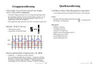
Oftmals werden time-hopping (TH) Verfahren angewandt. Dabei wird ein Symbol d
gemäß eines Kodes c in mehrere Chips aufgeteilt. Im (mittleren) Abstand Tf (pulse
repetition time) wird ein Chip, also der Sendepuls wT X (monocycle) der Breite
τW , übertragen, wobei ein Chipintervall TC lang ist (vgl. Abbildung 1). Vorrangig
dient TH dazu, mehrere Nutzer gleichzeitig im Netzwerk unterzubringen. Werden PN
(pseudo-random) Sequenzen verwendet, wird gleichzeitig das Spektrum des Sendesignals
geglättet. Da sich die Signalleistung des Pulses aus den akkumulierten Einzelleistungen
der Chips ergibt, können mit dieser Methode auch immer die von den Regulierungsbehörden
geforderten Leistungsmasken eingehalten werden.
Das mit dem Modulationsindex δ PPM-modulierte Sendesignal des k-ten Nutzers bei
Anwendung von TH kann dargestellt werden, vgl. auch [4]:
s (k)
T X (t) =
∞
i=−∞
wT X
t (k) − iTf − c (k)
i TC − δd (k)
⌊i/NS⌋ . (1)
Ein Symbol besteht aus NS Chips. Abbildung 1 veranschaulicht das Prinzip des
Time-Hopping bei Einsatz von PPM.
’0’ ’1’
τW
TC
Tf
Abb. 1. Time-Hopping Prinzip mit PPM-modulierten Signalen
Empfängerentwurf
Prinzipiell könnte man die gängigen UWB-Empfänger in Kanal-matched-filter (Kanal-
MF) und Energiedetektoren unterteilen. Als Spezialfall des Kanal-MF kann der Rake-
Empfänger betrachtet werden. Allerdings können beim Rake nur endlich viele Finger
implementiert werden. Damit können auch nur endlich viele Mehrwege berücksichtigt
werden. Da bei UWB-Übertragung eine große Anzahl an Mehrwegen zu erwarten ist,
müssen also sehr viele Finger implementiert werden, um möglichst viel Leistung ëinzusammelnünd
damit eine geringe Bitfehlerrate (BER) zu gewährleisten. Insbesondere
sind hohe BERs zu erwarten, wenn keine direkte Sichtverbindung (non-line-of-sight
NLOS) besteht, wie in [5] gezeigt wurde. Bei einem Kanal-MF muss vor dem Datenempfang
der Kanal geschätzt werden. Ist die Kanalschätzung perfekt, können alle
2

Mehrwegekomponenten bei der Demodulation berücksichtigt werden. Ein solcher Ansatz
wird z.B. in [6] zugrunde gelegt.
Die Komplexität eines Empfängers basierend auf dem Rake-Ansatz steigt mit der Anzahl
der Finger und ist für Empfänger mit geringem Leistungsverbrauch nicht geeignet.
Daher wird in Sensornetzwerken oftmals der Ansatz der Energiedetektion realisiert, so
z.B. in [3]. Dem Nachteil einer geringeren theoretischen Leistungsfähigkeit von Energiedetektoren
gegenüber Rake-Empfängern steht der Vorteil einer einfachen Realisierbarkeit
mittels Integratoren [2] gegenüber. Dabei ist keine Kanalschätzung nötig. Weiterhin
existieren vielversprechende Ansätze, bei denen unmodulierte Templates als Referenzsignale
gesendet werden, die dann mit den kurz darauffolgenden Daten korreliert
werden (auto-correlating receiver).
Kanalmodelle
Es gibt eine große Anzahl von Kanalmodellen für UWB-Signale [7], neue, auf niederbitratige
Übertragung zugeschnittene Modelle entstehen aktuell im Rahmen der Standardisierungsaktivitäten
von IEEE 802.15.4a. Viele greifen auf das Saleh-Valenzuela
(SV)-Modell zurück, welches auf Messungen im Innenbereich beruht [8]. Dabei werden
die Mehrwegekomponenten nicht mit einer statistischen Verteilungsfunktion beschrieben.
Vielmehr wird davon ausgegangen, dass in Gebäuden Reflexionen an Clustern
auftreten (z.B. eine Möbelgruppe), und typischerweise viele Cluster zu finden sind. Die
Ankunftszeiten von Echos innerhalb eines Cluster bezogens auf die Ankunftszeit des ersten
Echos des Clusters werden nun mit einem Poisson-Prozess der Rate λ beschrieben.
Die Ankunftszeit der ersten Echos der jeweiligen Cluster werden als Poisson-Prozess
mit der Rate Λ modelliert, τk bezeichnet die Ankunftszeit eines Pfades des l-ten Cluster
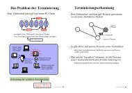
relativ zur Ankunftszeit des ersten Pfades des Clusters. Dies wird in Abbildung 2 verdeutlicht.
Die mittlere Leistung der einzelnen Pfade folgt einem exponentiellen Abfall.
Zusätzlich unterliegt jeder Pfad einem Rayleigh-Zufallsprozess.
Kanalleistung
Einhüllende
exp(−τl/γ)
exp(−t/Γ )
Cluster 1 Cluster 2 Cluster 3
Clustereinhüllende
Zeit
Abb. 2. Saleh-Valenzuela-Modell (nach [8])
LOS NLOS
Λ 0.025 ns −1 0.4 ns −1
λ 0.045 ns −1 5.5 ns −1
Γ 14.5 ns 14 ns
γ 8 ns 7.5 ns
Abb. 3. Parameter des
SV-Mehrwegekanals
Für die weiteren Untersuchungen wird das SV-Modell mit den in Abbildung 3 gegebenen
Parametern verwendet. Darin stellen Λ die Cluster Ankunftsrate, λ die Echo
Ankunftsrate, Γ den Cluster Dämpfungsfaktor und γ den Echo Dämpfungsfaktor dar.
3

3 Leistungsfähigkeit von IR in Sensornetzwerken
Im Folgenden sollen einige Simulationsergebnisse vorgestellt werden, die zur Beurteilung
der Leistungsfähigkeit von IR-UWB bei niederbitratiger Übertragung dienen. Dabei
wird davon ausgegangen, dass Sender und Empfänger perfekt synchronisiert sind
und der Empfänger perfekte Kanalkenntnis hat. Als Modulationsverfahren wird PPM
angewandt. Pro Rahmen wird ein Gauss’scher Monopuls der Dauer 1 ns ausgesendet
(also NS = 1). Es wird keine Interferenz mit anderen Systemen betrachtet. Als Kanalmodell
dient der SV-Kanal mit den in Tabelle 3 angegebenen Parameter.
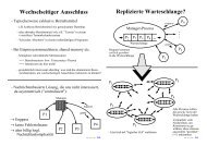
Zunächst wird ein Kanal-Matched-Filter (Kanal-MF) betrachtet und die Auswirkungen
der Rahmenlänge auf die Bitfehlerrate (BER) in einem single-link System (1 Sender, 1
Empfänger) betrachtet. Die Datenrate R ergibt sich aus der betrachteten Rahmenlänge
Tf mittels R = 1/Tf.
BER
10 −1
10 −2
10 −3
10 −4
10 −5
Rahmendauer: 1 ns
Rahmendauer: 2 ns
Rahmendauer: 3 ns
Rahmendauer: 5 ns
Rahmendauer: 10 ns
Rahmendauer: 100 ns
Referenz AWGN−Kanal
10
4 6 8 10 12
−6
SNRb [dB]
BER
10 −1
10 −2
10 −3
10 −4
10 −5
Rahmendauer: 1 ns
Rahmendauer: 2 ns
Rahmendauer: 3 ns
Rahmendauer: 10 ns
Rahmendauer: 100 ns
Rahmendauer: 500 ns
Referenz: AWGN−Kanal
10
4 6 8 10 12
−6
SNRb [dB]
Abb. 4. BER im LOS/NLOS (links/rechts) SV-Mehrwegekanal für versch. Rahmendauern Tf
Abbildung 4 zeigt die Ergebnisse für den SV-Kanal für LOS und NLOS. Offensichtlich
tritt bei geringen Rahmendauern aufgrund der Mehrwege Interpulsinterferenz (IPI)
auf, so dass eine Sättigung der Bitfehlerrate zu beobachten ist. Bei langen Rahmendauern
(> 100 ns) ist der Abstand zwischen 2 Pulsen gross genug, so dass der Einfluss von
IPI zu vernachlässigen ist.
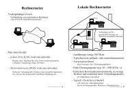
Im Folgenden wird die Leistungsfähigkeit eines Rake bei verschiedenen Fingeranzahlen
betrachet. Abbildung 5 bestätigt, dass bei UWB aufgrund der hohen Bandbreite
viele Mehrwege aufgelöst werden. Somit ist die Anzahl der zur Demodulation
benötigten Rake-Finger hoch.
Während im LOS-Fall aufgrund der starken LOS-Komponenten noch vernünftige Fehlerraten
mit wenigen Fingern erreicht werden können, ist die Leistungsfähigkeit von
wenigen Fingern im NLOS eindeutig nicht ausreichend, da damit zu wenig Leistung
eingesammelt wird. Damit scheidet ein Rake-Empfänger für Sensornetzwerke, die im
Innenbereich eingesetzt werden sollen, aufgrund des Hardwareaufwandes aus. Ähnliche
4

BER
10 0
10 −1
10 −2
10 −3
10 −4
10 −5
LOS / Fingerzahl: 1
LOS / Fingerzahl: 2
LOS / Fingerzahl: 3
LOS / Fingerzahl: 10
Referenz AWGN−Kanal
10
4 6 8 10 12
−6
SNRb [dB]
BER
10 0
10 −1
10 −2
10 −3
10 −4
10 −5
NLOS / Fingerzahl: 1
NLOS / Fingerzahl: 10
NLOS / Fingerzahl: 127
NLOS / Fingerzahl: 2032
Referenz: AWGN−Kanal
10
4 6 8 10 12
−6
SNRb [dB]
Abb. 5. BER im LOS/NLOS (links/rechts) SV-Kanal für versch. Anz. von Rake-Fingern
Ergebnisse wurden bereits in [9] dokumentiert. Darin wird u.a. gezeigt, dass in kritischen
Kanälen wesentlich mehr als 10 Finger benötigt werden, um eine vernünftige
BER zu erreichen.
Es bleibt die Leistungsfähigkeit von nicht-kohärenten Empfangsmethoden,d.h. Energiedetektion
zu untersuchen. Würde Energiedetektion eine gute BER erreichen, wäre
IR-UWB eine interessante Alternative zu herkömmlichen Schmalbandverfahren, da
dann Transceiver mit geringem Leistungsverbrauch realisierbar wären.
Literatur
1. FCC, “Report and order, FCC 02-48,” Apr. 2002.
2. L. Stoica, S. Tiuraniemi, H. Repo, A. Rabbachin, and I. Oppermann, “A low complexity UWB
circuit transceiver architecture for low cost sensor tag systems,” in Symp. on Personal Indoor
Mobile Communication, Sept. 2004, vol. 1, pp. 196–200.
3. I. Oppermann and et al., “UWB wireless sensor networks: UWEN-a practical example,” IEEE
Commun. Mag., vol. 42, pp. S27–S32, Dec. 2004.
4. M.Z. Win and R.A. Scholtz, “Impulse radio: How it works,” IEEE Communications Letters,
vol. 2, pp. 36–38, Feb. 1998.
5. J.D. Choi and W.E. Stark, “Performance of ultra-wideband communications with suboptimal
receivers in multipath channels,” IEEE J. Select. Areas Commun., vol. 20, pp. 1754–1766,
Dec. 2002.
6. F. Ramírez-Mireles, “On the performance of ultra-wide-band signals in Gaussian noise and
dense multipath,” IEEE Transactions on Vehicular Technology, vol. 50, pp. 244–249, Jan.
2001.
7. J. Foerster and Q. Li, “UWB channel modeling contribution from intel,” in IEEE P802.15-
02/279r0-SG3a, Nov. 2003.
8. A.A.M. Saleh and R.A. Valenzuela, “A statistical model for indoor multipath propagation,”
IEEE J. Select. Areas Commun., vol. SAC-5, pp. 128–137, Feb. 1987.
9. Y. Ishiyama and T. Ohtsuki, “Performance comparison of UWB-IR using rake receivers in
UWB channel models,” in 2004 International Workshop on Ultra Wideband Systems (Joint
UWBST&IWUWBS 2004), 2004, pp. 226–230.
5

Using TinyOS on BTnodes
Jan Beutel, Attila Dogan
Computer Engineering and Networks Laboratory
Department of Information Technology and Electrical Engineering
ETH Zurich, Switzerland
beutel@tik.ee.ethz.ch, adogan@ee.ethz.ch
Abstract. TinyOS has been very popular for wireless sensor network
applications and is a de facto standard today. This study compares the
architectural differences between the BTnode and Mote platforms and
explains how to implement TinyOS applications on the BTnodes. In
addition this enables to interface between networks of Mote and BTnode
devices.
1 Introduction
Starting out from an all-in-one Bluetooth module, the BTnode family of nodes
has matured to a full fledged dual radio wireless networking platform with both
a Bluetooth and a Chipcon CC1000 low-power radio [2]. Thus, the BTnode rev3
is a twin, of the Berkeley Mica2 Mote [5] and the previous BTnode rev2 and
ideally suited to interface between both classes of devices. Both radios can be
operated simultaneously or be independently powered off completely when not
in use, considerably reducing the idle power consumption of the device.
This new architecture opens new opportunities to interface between ultralow-power
devices like the Berkeley Motes and larger devices such as Bluetoothenabled
appliances [4], or to investigate duty-cycled multi-frontend devices with
wake-up radios [7] or bandwidth–power–latency trade-offs.
This study provides a base for the implementation of TinyOS [3] applications
on the BTnode platform. A short synopsis of the architectural differences of the
BTnode and Mote platforms is followed by a basic introduction to TinyBT, the
TinyOS support for BTnodes.
2 BTnode Hardware
The BTnode hardware is built around an Atmel ATmega128L microcontroller
with on-chip memory and peripherals (see Fig. 1). The microcontroller features
an 8-bit RISC core delivering up to 8 MIPS at a maximum clock frequency of
8 MHz. The on-chip memory consists of 128 kbytes of in-system programmable
Flash memory, 4 kbytes of SRAM, and 4 kbytes of EEPROM. There are several
integrated peripherals: JTAG for debugging, timers, counters, pulse-width modulation,
10-bit analog-digital converter, I2C bus, and two hardware UARTs. An
6

Low-power
Radio
Bluetooth
System
GPIO Analog Serial IO
ATmega128L
Microcontroller
Power Supply
SRAM
LEDs
Fig. 1. BTnode rev3 hardware architecture overview.
external low-power SRAM adds an additional 240 kbytes of data memory to the
BTnode rev3 system [1].
An assessment of the platform status and the experience gained through
applications implemented on the BTnode rev2 resulted in the following design
criteria that were realized in the BTnode rev3:
– Enhanced Bluetooth 1.2 subsystem supporting multiple-master Scatternets
– Additional low-power radio
– Integrated, battery-powered power supply
– Switchable power supplies for radios
– Board-to-board extension connector
– Open interface documentation of radios (developer information)
Fig. 2. The BTnode rev3 hardware with an AVR core, a CC1000 radio and a ZV4002
Bluetooth device in a Mica2 form factor.
2.1 Hardware Details – The BTnode rev3 Compared
The basic differences in the hardware architecture of the BTnode rev3 and the
Mica2 Mote are outlined in Table 1. The main architectural advantages are the
7

dual radio, the extended data memory and the power switches for the radios
that provide the application developer with more resources and flexibility while
maintaining the basic Mica2 Mote characteristics. An additional address latch
and 3 GPIO lines are used to multiplex the storage memory, the LEDs and the
power switches to the AVR memory bus. This extra functionality adds some
complexity that needs to be supported by the respective device drivers as well
as in the applications.
Platform BTnode rev3 Mica2 Mote
Bluetooth Zeevo ZV4002 none
Low-power radio CC1000 CC1000
Data Memory 64 kB 4 kB
Storage 180 kB SRAM 512 kB Flash
LEDs 4 3
Serial ID no yes
Debug UART UART0 UART0, UART1
Connector Molex 15 Pin or Hirose DF17 40 Pin Hirose DF9 51 Pin
Regulated power supply yes, 2xAA cells or DC input none
Switchable power for radios yes
and extensions
none
Table 1. BTnode rev3 hardware details compared to the Mica2 Mote.
3 TinyOS on BTnodes – TinyBT
A first step to support TinyOS on the BTnode platform was achieved by the
Manatee project [6] that developed portions of a Bluetooth protocol stack
for TinyOS and an initial platform description of the BTnode for TinyOS
that is available under /tinyos-1.x/contrib/tinybt and documented under
http://www.distlab.dk/madsdyd/work/tinyos. Similarly, the Intel imote effort
[4] has created a proprietary Bluetooth stack that uses TinyOS (available under
/tinyos-1.x/beta/platform/imote. Both these efforts are not completely
compatible with the BTnode rev3 but can be used as a reference for further
work.
The current support for the BTnode rev3 in TinyOS is integrated into
TinyBT where a platform definition as well as device specific drivers can be
found. These allow to compile and run simple TinyOS demo applications like
CntToRFM, RFMToLED, Surge, etc. that rely on the CC1000 radio.
A simple application using the AVR core and the CC1000 radio needs to
import the platform specific hardware.h file and initialize the power for the
CC1000 radio. This is done using the set_latch() function that controls the
multiplexed lines for the power switches and LEDs that is automatically included
when the btnode3_2 platform is selected as compile target by make btnode3_2.
8

For the application programmer, everything looks just as if writing a TinyOS
example for any other target platform. If applications want to make use of other
specialized features of the BTnode rev3 like the extended storage memory or
a combination of the two radios, specific operating strategies and software will
need to be developed.
Fig. 3. The Surge demo application running on a mixed network of Mica2 Motes (nodes
0, 1 and 2) and BTnodes (nodes 4 and 5).
4 Summary
In this study we have investigated the feasibility of using TinyOS on the
BTnode rev3 platform. A basic set of drivers and a platform definition has
been created and tested with simple demo applications. A heterogeneous network
consisting of Mica2 Motes and BTnodes has been created using the Surge
demo application (see Fig. 3).
Today TinyOS does not incorporate multiple threads and many abstractions
are oriented towards dataflow oriented interfaces which pose problems when
dealing with a packet oriented radio interface such as Bluetooth. The ongoing
work on the 2nd generation TinyOS (TinyOS 2.0 working group) as well as the
architectural advantages of the BTnode rev3 allow to explore novel applications
and flexible operating system concepts using dual radios and advanced power
saving techniques.
For further information please refer to http://www.btnode.ethz.ch and the
TinyOS developer resources found at http://www.tinyos.net/.
9

Acknowledgements
The work presented in this paper was supported (in part) by the National Competence
Center in Research on Mobile Information and Communication Systems
(NCCR-MICS), a center supported by the Swiss National Science Foundation
under grant number 5005-67322.
References
1. J. Beutel, M. Dyer, M. Hinz, L. Meier, and M. Ringwald. Next-generation prototyping
of sensor networks. In Proc. 2nd ACM Conf. Embedded Networked Sensor
Systems (SenSys 2004), pages 291–292. ACM Press, New York, November 2004.
2. J. Beutel, O. Kasten, F. Mattern, K. Römer, F. Siegemund, and L. Thiele. Prototyping
wireless sensor network applications with BTnodes. In Proc. 1st European
Workshop on Sensor Networks (EWSN 2004), volume 2920 of Lecture Notes in
Computer Science, pages 323–338. Springer, Berlin, January 2004.
3. D. Culler, J. Hill, P. Buonadonna, R. Szewczyk, and A. Woo. A network-centric
approach to embedded software for tiny devices. In First Int’l Workshop on Embedded
Software (EMSOFT 2001), volume 2211 of Lecture Notes in Computer Science,
pages 114–130. Springer, Berlin, October 2001.
4. J.L. Hill, M. Horton, R. Kling, and L. Krishnamurthy. Wireless sensor networks:
The platforms enabling wireless sensor networks. Communications of the ACM,
47(6):41–46, June 2004.
5. J.L. Hill, R. Szewczyk, A. Woo, S. Hollar, D. Culler, and K. Pister. System architecture
directions for networked sensors. In Proc. 9th Int’l Conf. Architectural Support
Programming Languages and Operating Systems (ASPLOS-IX), pages 93–104. ACM
Press, New York, November 2000.
6. M. Leopold, M.B. Dydensborg, and P. Bonnet. Bluetooth and sensor networks: A
reality check. In Proc. 1st ACM Conf. Embedded Networked Sensor Systems (SenSys
2003), pages 103–113. ACM Press, New York, November 2003.
7. E. Shih, P. Bahl, and M. Sinclair. Wake on Wireless: An Event Driven Energy
Saving Strategy for Battery Operated Devices. In Proc. 6th ACM/IEEE Ann. Int’l
Conf. Mobile Computing and Networking (MobiCom 2001), pages 160–171. ACM
Press, New York, September 2002.
10

A Collision-Free MAC Protocol for
Sensor Networks using Bitwise “OR”
1 Introduction
Matthias Ringwald, Kay Römer
Dept. of Computer Science
ETH Zurich, Switzerland
{mringwal,roemer}@inf.ethz.ch
Many widely used Medium Access Control (MAC) protocols for sensor networks
are based on contention, where concurrent access to the communication channel
by multiple sensor nodes leads to so-called collisions. Collisions are a source
of many undesirable properties of these MAC protocols such as reduced effective
bandwidth, increased energy consumption and indeterministic data delivery.
Hence, collisions are commonly considered a “bad thing”, and MAC protocols
strive to avoid them wherever possible. In sensor networks, communication activity
is typically triggered by an event in the physical world. In dense networks,
such an event triggers communication activity at many collocated nodes almost
concurrently, such that a high probability of collisions must be expected.
In this paper, we adopt another, more positive view on collisions. In particular,
we show that a set of synchronized nodes can concurrently transmit data,
such that a receiver within communication range of these nodes receives the bitwise
“or” of these transmissions. Based on this communication model, we can
provide efficient parallel implementations of a number of basic operations that
form the foundation for BitMAC: a deterministic, collision-free, and robust MAC
protocol that is tailored to dense sensor networks, where nodes report sensory
data over multiple hops to a sink.
2 Basic Assumptions
In this section, we present our communication model and characterize the class
of applications, for which BitMAC has been designed.
Our work is based on the assumption, that a node receives the “or” of the
transmissions of all senders within communication range. In particular, if bit
transmissions are synchronized among a set of senders, a receiver will see the bitwise
“or” of these transmissions. This behavior can actually be found in practice,
e.g., for radios that use On-Off-Keying (OOK), where ”1”/“0” bits are transmitted
by turning the radio transmitter on/off. BitMAC will use this communication
model only for a limited number of control operations. For the remainder (e.g.,
payload data transmission), other, perhaps more efficient modulation schemes
can be used if supported by the radio.
11

Furthermore, our work assumes that the radio supports a sufficient number
of communication channels, such that nodes within communication range can
switch to different channels to avoid interference.
BitMAC is designed for data-collection sensor networks, where many densely
deployed sensor nodes report sensory data to a sink across multiple hops. Data
communication is mostly uplink from the sensor nodes to the sink, although
the sink may issue control messages to the sensor nodes. One prominent example
of this application class are directed diffusion [2] and TinyDB [5]. Many
concrete applications (e.g., [1, 4, 6, 8]) show this behavior as well. Furthermore,
it is assumed that the network topology is mostly static. That is, after initial
deployment, node mobility and addition are rare events.
3 Protocol Overview
BitMAC is based on a spanning tree of the sensor network with the sink at the
root. In this tree, every internal node and its direct children form a star network.
That is, the tree consists of a number of interconnected stars. Within each star,
time-division multiplexing is used to avoid interference between the children
sending to the parent. Time slots are allocated on demand to nodes that actually
need to send. Using a distributed graph-coloring algorithm, neighboring stars are
assigned different channels as to avoid interference between them. Both the setup
phase and actual data transmission are deterministic and free of collisions.
In the following sections we will describe interesting parts of the protocol
with increasing level of complexity. We will begin with basic techniques for communication
among a set of child nodes and a parent node in a star network. We
will then discuss the part of the MAC protocol used to control a single star.
Finally, we will describe how these stars can be assembled to yield the complete
multi-hop MAC protocol.
(a)
(b)
Fig. 1. (a) Star network with a single parent. (b) Multiple stars with shared children.
4 Integer Operations
Let us assume that all or a subset of children need to transmit k-bit unsigned
integer values to the parent as depicted in Figure 1(a), where the latter is interested
in various aggregation operations (OR, AND, MIN, MAX) on the set of
values of the children.
12

Obviously, a bitwise “or” can be implemented by having the children synchronously
transmit their values bit by bit.
In order to compute MAX, the binary countdown protocol is used which
requires k communication rounds. In the i-th round, all children send the i-th
bit of their value (where i = 0 refers to the most significant bit), such that
the parent receives the bitwise “or”. The parent maintains a variable maxval
which is initialized to zero. When the parent receives a one, it sets the i-th bit
of maxval to one. The parent then sends back the received bit to the children.
Children stop participation in the algorithm if the received bit does not equal
the i-th bit of their value as this implies that a higher value of another child
exists. After k rounds, maxval will hold the maximum among the values of the
children. Note that children who sent the maximum will implicitly know, since
they did not stop participation. If the values are distinct among the children,
this operation implements an election.
In a parallel integer operation, parents of multiple stars that share one or
more children perform the same integer operation as depicted in Figure 1(b).
If all involved nodes are synchronized, all of the above integer operations can
be performed (synchronously) in parallel. For the OR and AND operations, our
communication model will ensure that all parents will obtain the correct result
for their respective children. For MAX, the parent will in general not obtain the
correct result. However, this operation implements an election, where any two
elected nodes do not share a common parent, if their values are distinct.
5 Star Network
Using the bitwise “or” operation, we present a MAC protocol for star networks,
which will be used as a building block for the multi-hop protocol presented in the
following section. Time-division multiplexing is used to avoid collisions and to
ensure a deterministic behavior of the protocol. In order to optimize bandwidth
utilization, time slots are allocated on demand to nodes that actually need to
send data.
Let us assume for the discussion that children have been assigned small,
unique integer IDs in the range 1...N. We will show in Section 6 how these can
be assigned. The protocol proceeds in rounds with the parent acting as a coordinator.
A round starts with the parent broadcasting a beacon message to the
children. Then children will transmit send requests to the parent. After receiving
these requests, the parent constructs a schedule and broadcasts it to the children.
During their time slots, children send their payload data to the parent.
The parent will then acknowledge successful receipt. If transmission failed, the
affected children will try a retransmission in the next round. For the send requests
and the acknowledgments, a bit vector of length N is used. As a further
optimization, the acknowledgment set can be concatenated with the beacon of
the following message as depicted in Figure 2.
13

Parent
Child 1
Child 2
Child 3
Preamble SOP ACK i−1
1
1
Sched i
Preamble SOP Data
Preamble SOP Data
Fig. 2. Round i of the optimized MAC protocol for star networks.
6 Multi-Hop Network
We now show how to extend the protocol for star networks to a multi-hop network.
First, nodes with the same hop count to the sink form rings. This is
achieved by flooding of a beacon message that contains a hop counter. This operation
is only possible because all nodes on ring i synchronously transmit the
beacon to nodes in ring i + 1 utilizing the bitwise “or” of the channel.
Next, the connectivity graph as shown in Figure 3(a) has to be transformed
into a spanning tree by reducing the number of uplinks of each node to one by
assigning separate radio channels. We will show in the next section how these
are assigned. After the channel assignment, each internal node and its direct
children form a star that uses the protocol presented in the previous section.
(a)
1 2 3
B C
Fig. 3. Distance from the sink (•) imposes a ring structure on the network. Network
links between nodes in the same ring are not shown.
7 Assigning Channels and IDs
In order to turn the hierarchical ring structure into a tree, each node must be
assigned to a single parent. A parent in ring i then must share a channel with
its children in ring i + 1, such that no other parent in ring i of the children uses
the same channel. More formally, this requires the assignment of small integers
(i.e., channel identifiers) to nodes in ring i, such that nodes who share a child in
ring i + 1 are assigned different numbers.
14
A
(b)
D
i−1
i
i+1

We assumed in Section 5 that children of a single parent are assigned small
unique integer numbers. With respect to the ring structure, this task can be
formulated as assigning small integers to nodes in ring i, such that nodes who
share a parent in ring i − 1 are assigned different numbers.
The above two problems can be combined into a two-hop graph coloring
problem: assign small integers (i.e., colors) to nodes in ring i, such that nodes
with the same number do not share a common neighbor in ring i − 1 or i + 1.
Note that common neighbors in ring i are not considered. In Figure 3(b), a valid
color assignment would be A = D = 1, B = 2, C = 3.
In order to solve this coloring problem, let us assume that a small number C
is known, such that the numbers 1...C (the color space) are sufficient to solve the
coloring problem. Simulation of random graphs in [7] has shown that choosing
C to be greater than two times the average node degree is sufficient with high
probability. In practice, C will be set to the number of available radio channels.
Under these assumptions, we can use a deterministic variant of the algorithm
presented in [3] to solve the above described two-hop graph coloring problem for
ring i. For this algorithm, each node in ring i maintains a set P (the palette) of
available colors, which initially contains 1...C. The algorithm proceeds in rounds.
In each round, every node in ring i selects an arbitrary color c from its palette P .
Some nodes may have selected conflicting colors. For each possible color, at most
one node in a two-hop neighborhood is allowed to keep its color. All other nodes
must reject the color and remove it from P . The process of selecting nodes that
keep their color is implemented by using the parallel MAX operation described
in Section 4 where at most one node is chosen from a two-hop neighborhood. As
a unique value, a 16-bit MAC address can be used.
The algorithm requires at most C rounds. It is important to note that this
algorithm can be performed by every fourth ring in parallel, hence, the whole
network can be colored in 4C rounds.
8 Further Issues
There are several further issues that cannot be described in detail in this extended
abstract. Some are explored in the full paper [7], for example, time
synchronization, dealing with bit errors, and topology changes. In [7] we also
analyze setup time and energy efficiency of the protocol. Other issues will be
evaluated in future experiments such as robustness against interference and link
fluctuations.
9 Conclusion
We have presented BitMAC, a deterministic, collision-free, and robust protocol
for dense wireless sensor networks. BitMAC is based on an “or” channel, where
synchronized senders can transmit concurrently, such that a receiver hears the
bitwise “or” of the transmissions.
15

10 Acknowledgments
The work presented in this paper was supported (in part) by the National Competence
Center in Research on Mobile Information and Communication Systems
(NCCR-MICS), a center supported by the Swiss National Science Foundation
under grant number 5005-67322.
References
1. R. Beckwith, D. Teibel, and P. Bowen. Pervasive Computing and Proactive Agriculture.
In Adjunct Proc. PERVASIVE 2004, Vienna, Austria, April 2004.
2. C. Intanagonwiwat, R. Govindan, and D. Estrin. Directed Diffusion: A Scalable and
Robust Communication Paradigm for Sensor Networks. In 6th Intl. Conference on
Mobile Computing and Networking (MobiCom 2000), Boston, USA, August 2000.
3. Öjvind Johannson. Simple Distributed ∆ + 1 Coloring of Graphs. Information
Processing Letters, 70:229–232, 1999.
4. C. Kappler and G. Riegel. A Real-World, Simple Wireless Sensor Network for Monitoring
Electrical Energy Consumption. In EWSN 2004, Berlin, Germany, January
2004.
5. S. R. Madden, M. J. Franklin, J. M. Hellerstein, and W. Hong. TAG: a Tiny
Aggregation Service for Ad-Hoc Sensor Networks.
December 2002.
In OSDI 2002, Boston, USA,
6. R. Riem-Vis. Cold Chain Management using an Ultra Low Power Wireless Sensor
Network. In WAMES 2004, Boston, USA, June 2004.
7. M. Ringwald and K. Römer. BitMAC: A Deterministic, Collision-Free, and Robust
MAC Protocol for Sensor Networks.
2005.
In EWSN 2005, Istanbul, Turkey, January
8. R. Szewczyk, J. Polastre, A. Mainwaring, and D. Culler. Lessons from a Sensor
Network Expedition. In EWSN 2004, Berlin, Germany, January 2004.
16

Energy Reduction Strategies for Sensor-Node-on-a-Chip
The SNoC Project at the University of Freiburg
1 Introduction
Y.Manoli, S.Ramachandran, S.Jayapal, S.Bhutada, R.Huang
Institute of Microsystem Technology (IMTEK),
Chair of Microelectronics,
University of Freiburg, Germany.
{manoli@imtek.de}
A wireless sensor network is a cluster of sensor nodes communicating with each
other, for collecting, processing and distributing data. Each sensor node consists of
sensors, data converters, a processor, power management unit, radio for wireless
communication and networking. Wireless sensor networks have a wide range of
applications like air traffic control, video surveillance, industrial and manufacturing
automation, distributed robotics, smart textiles, building, structure as well as
environmental monitoring etc. A wireless sensor network may be small or large
depending on the application requirements. However, the ubiquitous wireless
network of micro-sensors is changing the world of sensing, computation and
communications.
The goal of the SNoC project at University of Freiburg is to develop energy
reduction strategies and to design all the necessary electronics of a sensor node on a
single chip thus ensuring a low power operation of the system while also reducing the
overall size of the node.
1.1 Sensor Node on a Chip
The general architecture of a sensor node is shown in figure (1). It has one or more
sensors, an application specific dedicated logic unit to process and control the data, a
RF modem with DSP engine to send and receive message to and from other sensor
nodes or base station in the network and a battery or other energy source to provide
power for all execution units on the node.
These different building blocks can be implemented using standard off-the-shelf
components. This provides the flexibility of rapidly implementing a system
prototype. But commercially available sensor nodes are not always optimized for
power. Although most micro-controllers have various power-down and idle modes
they still tend to consume large amounts of power. Even at a moderate speed of
17

1 MHz they require microwatts of power in the power down and milliwatts in the
active mode [1]. These general purpose devices are designed with flexibility in mind
and less for low-power requirements. They include a number of functional units
(serial and parallel interfaces, keyboard and display control etc) that in the context of
a sensor node might not be required but still contribute to the power consumption.
Designing a dedicated chip on the other hand allows the optimization of the
architecture for low-power requirements. This mixed signal system can include
sensor interface electronics leading to greater area and power savings. One
disadvantage is of-course the longer design time. For evaluation purposes FPGA and
FPAA solutions can be implemented providing the functionality but of-course at a
much higher power level.
The following sections discuss different possibilities of energy reduction in the
computation and communication modules.
Sensor Array
RF MODEM
With
DSP Engine
Application
Specific Dedicated
Logic Unit
Battery/Energy
source
Figure 1. General architecture of SNoC.
2. Energy Reduction at different Levels of Abstraction
Optimization of power can be done at different levels of abstraction viz.,
behavioural, architectural and logical or physical levels. In the behavioural and
architectural level optimization can bring 10% to 90% power savings [2]. This is
because any changes made at this level will be reflected at the lower levels of
abstraction. So a very careful design of each and every module is necessary.
Dedicated hardware for low level tasks and careful use of software for high level
tasks reduces the energy at the architectural level while dynamic energy scaling
schemes reduce the power at the logic and circuit level.
This section describes the Characteristics of Sensor-Node-On-a-Chip, the
hardware software co-design methodology and energy efficient LSI design in sections
(2.1), (2.2) and (2.3) respectively.
18

2.1 Characteristics of SNoC:
There are many challenges to be faced in designing energy efficient computation
and communication building blocks and developing algorithms for adhoc networking
for wireless sensor nodes. The first challenge is that all nodes are energy constrained.
So, if the numbers of nodes are increased, it becomes infeasible to replace all of the
batteries of the sensors. To prolong the lifetime of the sensor nodes, all aspects of the
sensor system operation should be energy efficient. So, the energy requirement
depends on the state of operation, like standby or active mode and the nature of
applications. But, in most of the applications, the standby mode will be longer than
the active operating time (Figure 2).
Power
Time
Active mode
Standby mode
Figure 2. Power required versus operating time
A wireless sensor network node is a system which has long idle times. This means
that the node in the network does not accumulate, send or receive data very often.
Most of the time the system can be in the sleep state. When there is a request from
other nodes or from the sensors on the system then only a part of the system wakes
up, executes some task and goes to sleep again. When a sensor on a node reads some
new value from the environment it does not necessarily transmit the data to the
master node or any other node in the network, unless the data is critical. The system
can ignore the new data or can store it for future transmission.
The node has a number of different operating modes for reducing the power
consumption. As mentioned above the wake-up/active time is much less than the
sleep/power down time. This forces the design of SNoC to be also optimized for the
sleep state power consumption. A number of different sleep modes maintain only the
blocks required for a specific background task active. Dedicated sensor data
acquisition hardware collect data or compare them to critical values without the
intervention of the central processing unit.
A novel microprocessor architecture, which was especially designed to reduce
power dissipation of modern system-on-a-chip, was introduced in [3]. This paper
introduces new type of data storage files and hardware supported constant elimination
to utilize the mostly local scope of common arithmetic operations for reducing
energy. A multi-level instruction-cache scheme together with a cache controller
supporting sophisticated opcode pre-processing operations like Huffmann decoding
decreases the amount of external memory access and size. Additionally the width of
pointers is significantly reduced by a table-lookup cache miss concept. Finally a
19

segmented gray-code program counter decreases the switching activity on the address
bus by an average of 25-30% [4].
2.2 Hardware software co-design approach
Due to the growing complexity of embedded systems new design methodologies and
concepts are mandatory. First of all, the design process must be shifted towards
higher levels of abstraction. Therefore a focus is set upon a system-level design
methodology. The section (2.2) shows an approach to hardware-software co-design
for design of low power Wireless sensor nodes.
Co-design may include integrated synthesis of hardware and software components,
which we refer to as hardware/software co-synthesis [5]. Automated
hardware/software co-synthesis may allow the designer to explore more of the design
space by dynamically reconfiguring the hardware and software to find the best overall
organization as the design evolves. This can lead to better results than could be
achieved if the hardware and software architectures had to be specified up-front,
during the early stages of the design.
Design tools for hardware/software co-synthesis must understand the relationship
between the hardware and software organization and how design decisions in one
domain affect the options available in the other. It also requires an understanding of
how the overall system cost and performance are affected by the hardware and
software organization.
Hardware
Synthesis
Specification
Architecture allocation
Application Mapping
Activity (Task) Scheduling
Energy Management
Evaluation
Software
Synthesis
Figure 3. System-Level Co-Synthesis flow
20

Co-synthesis is the process of deriving a mixed hardware-software implementation
from an abstract functional specification of the system. To achieve this goal, the cosynthesis
needs to address four fundamental design problems: architecture allocation,
application mapping, and task scheduling and most important in this case energy
management [6]. Figure (3) shows the co-synthesis flow in diagrammatic form. The
energy management techniques we can apply to wireless sensor nodes is dynamic
voltage scaling and optimizing each step for energy, area and cost, then evaluating
and going back to steps in the flow. After evaluation of the system according to the
requirements, we can finally proceed to hardware and software synthesis.
2.3. Energy Efficient Large Scale Integration Unit.
The process technology scaling requires a reduction of the supply voltage and
threshold voltage. In the nanometer regime, the static leakage power component starts
dominating the switching power in the highly integrated applications [7]. Due to the
technology limitations, designing energy efficient Microsystems in deep sub micron
technologies becomes a challenging task. Sections (2.3.1) and (2.3.2) discuss how
energy reduction techniques can be implemented in an autonomous wireless sensor
node. Figure (2) shows that a major portion of the precious battery lifetime is mostly
wasted in standby mode. So, designing a system which reduces both the standby and
active power is most important for the wireless sensor node.
2.3.1 Energy Constrained Sensor System
Energy efficient LSI design maximizes the useful lifetime of the battery source,
by adjusting the supply and threshold voltage. The supply voltage scaling is a well
known method of reducing the energy per operation with or without performance
penalty based on the application requirements. For autonomous wireless sensor
systems, the energy is usually much more important than performance requirements
[8]. So, the total energy requirements depends on the state of operation as shown
Total Energy = f (E [active mode], E [standby mode]) (1)
To reduce the total energy, both active and standby mode energy reduction is
necessary. The proposed architecture is discussed in detailed in section (2.3.2)
2.3.2 Dynamic Energy Scaling
We propose the dynamic energy scaling (DES) technique by which the supply and
threshold voltage is varied by constantly maintaining the performance of the system
for burst mode computation based on the temperature and process variations. The
change in the threshold voltage depending on the change in the supply voltage results
in a constant performance with less switching power. The threshold voltage varies
either due to the ambient temperature or by process variations. By employing a body
21

ias potential, the active and standby power can be reduced at the lowest possible
value at an optimal performance.
The conventional dynamic voltage scaling technique reduces the supply
voltage based on the performance demands, but it does not taken into account the
leakage power and ambient temperature [9]. In our DES scheme, energy is altered
dynamically based on the fixed performance and process variations. This technique
leads to switching and standby energy reduction as shown in Figure (4)
During the active mode of operation, the supply voltage is reduced while the
threshold voltage is also reduced by changing the forward body voltage thus
maintaining the performance of the system constant. Through this technique, the
switching power of the system is decreased while maintaining the same performance
as with a high supply voltage and still having the leakage power at a low level.
Temperature
sensor
Performance
Tracking
System
During the standby mode, withdrawing the body bias voltage or even applying a
reverse body bias increases the threshold voltage which in turn reduces the standby
leakage power of the sensor system.
3. Communication module
Body Bias
generator
Voltage
Regulator
Feedback
Loop
The communication is a very important design issue in a wireless sensor network
(WSN) because it primarily determines the reliability of network connections and
data exchanging between different nodes. Moreover it consumes much energy for
data and message exchanging. There are many variations for the wireless
communication means which can be used in WSN. They are electromagnetic (EM)
wave, magnetic field, ultra sonic and optics. These methods are suitable for different
application scenarios according to their properties.
Radio frequency (RF) has many advantages over other transmission means.
Simplicity for transmitting and receiving is obvious. The signal which is propagated
in space can be transmitted to and received by antenna, which is as simple as a metal
wire or different shapes of metal structures. RF can use a wide range of frequencies,
Vbn
Vbp
VDD
Figure.4. Dynamic Energy Scaling
22
Target LSI

theoretically from zero to infra-red. Therefore, the bandwidth of RF is much wider
than the ultra sonic and magnetic field. RF can also penetrate many obstacles and can
transmit a very long distance by an electromagnetic energy.
In WSN, as in commercial mobile networks, it is very important to develop a
technique to avoid interference between communication links. Generally, different
radio resource management plans can be used to share the limited frequency
spectrum. For instance, frequency-division-multiple-access isolates different
communication links to specific frequency bands to avoid the interference. Likewise,
time-division-multiple-access separates different communication links in different
time slots. Code-division-multiple-access, a more advanced technique, overcomes the
interference between communication links by allocating different spread spectrum
sequences to different units. In present years, space division technology, which uses
the smart antenna, is an interesting research topic. Although this technology needs
more complex circuits and antenna structures, it seems to give some promising
features to WSN, such as localization and route computing [10] [11].
These various technologies are always implemented in different specifications. As
shown in the table 1, there are 3 different protocols which are being or can be used in
wireless personal area network (WPAN) and also are a good choice for the WSN.
Bluetooth is popularly used in wireless sensor network because much hardware and
software are available from many companies. However, this protocol is not designed
for the low data rate scenario and WSN, as claimed by the ZigBee developers and its
power efficiency is not sufficient as required by a wireless sensor network. ZigBee is
especially designed for low data rate wireless personal area network and uses IEEE
802.15.4 protocol as physical and MAC layer specification. ZigBee seems to be a
good candidate for the wireless sensor network and it attracts more and more
attention from different companies and institutes. Ultra wide band is a new
technology which is just appearing. The specific modulation scheme of ultra wide
band is still undefined. Furthermore, the interference from ultra wide band to other
electronic modules, for instance GPS, is still under research. Table 1 summarizes
different protocols' specifications.
In WSN, the energy efficiency is an important design issue. Therefore, the system
design and circuit design is optimized for low power while maintaining the necessary
performance. Bearing this in mind, the system uses the receive signal strength
indication in the receiver node and programmable power amplifier in the transmission
node to control the transmission power for different communication ranges. The
system also uses RF energy detection circuit to monitor the received signal and wake
up the node control system when the signal is over the control threshold level set by
the software.
4. Conclusion
This paper has discussed the Sensor-Node-On-a-Chip project at the Albert-
Ludwig-University, Freiburg. It has been shown that an application specific design
using dedicated hardware for the low level tasks and careful use of software for high
23

level tasks can reduce the power consumption at the architectural level. An optimized
communication link as well as dynamic voltage scaling can reduce the power at the
logic and circuit level.
Table 1. Different communication protocols and their specifications
Protocols Frequency (MHz) Modulation
Channel
Bandwidth
(MHz)
Channels
Data rate
(kb/s)
Bluetooth 2400-2483.5 GFSK 1 79 765
ZigBee
Ultra-Wide
Band
References
2400-2483.5 O-QPSK 5 16 250
902-928 BPSK 2 10 40
868-868.6 BPSK 1 1 20
3100-10600 Un-defined 3000 1 100,000
[1]Gerald Kupris, Freescale solution for IEEE 802.15.4/Zigbee June 2004,
IEEE802.15.4/zigbee workshop, Loerach, Germany
[2]Gailhard, N.Julien, J.-Ph.Diguert, E.Martin, How to transform an Architectural Synthesis
tool for Low Power VLSI Designs
[3]Hakenes, R., Manoli, Y.A Segmented Gray Code for Low-Power Microcontroller Address
Buses EUROMICRO 99, Workshop on Digital System Design, 1999. EUROMICRO 99.
Proceedings. Volume 1, 1999, 240-243
[4]Hakenes,R.,Manoli,Y. A Novel Low Power Microprocessor Architecture
International Conference on Computer Design (2000) Proceedings, 2000, 141-146
[5]Jay K. Adams, Donald E. Thomas The Design of Mixed Hardware/Software Systems in
proc.33rd DAC’96, 1996.
[6]M. T. Schmitz, B. M. Al-Hashimi, P. Eles, System-level design techniques for energyefficient
embedded systems Kluwer Academic Publishers, Feb. 2004.
[7]Shekhar Borkar, Intel Fellow and Director, Intel Corp., Hillsboro, OR Low-Voltage
Design for Portable Systems, IEEE I ISSCC 2002.
[8]Ian F.Akyildiz, Weilian Su, Yogesh Sankarasubramaniam, and Erdal Cayirci, A survey on
Sensor Networks IEEE Commmunication magazine 2002
[9]T.Burd, T.Pering,A.Stratakos,R.Brodersen, A Dynamic Voltage-Scaled Microprocessor
System, 2000 IEEE International Solid-State Circuits Confreence Digest of Technical
Papers, Feb 2000.
[10]Huang R., Manoli Y., Power Efficiency in Wireless Sensor Networks using Directional
Antennas , VDE-Kongress 2004 Conference on Ambient Intelligence, Berlin, 2004
[11]Huang R., Manoli Y., Phased Array and Adaptive Antenna Transceivers in Wireless
Sensor Networks, EUROMICRO Symposium on Digital System Design (DSD 2004),
Renne, France, 2004,
24

Deployment Support
for Wireless Sensor Networks
Matthias Dyer, Jan Beutel, and Lennart Meier
Computer Engineering and Networks Laboratory, ETH Zurich, Switzerland
{dyer,beutel,meier}@tik.ee.ethz.ch
Abstract. We present the concept of Deployment-Support Networks
(DSN), a tool for the coordinated deployment of distributed sensor networks.
A DSN supports the development, debugging, monitoring, and
testing of sensor–network algorithms and applications. With our implementation
of the DSN on the BTnode rev3 platform, we have proven
that the concept scales well to a large number of nodes.
1 Introduction
The recent focus on wireless sensor networks (WSNs) has brought about many
different platforms such as the BTnodes [1] or the Berkeley Motes [2]. Researchers
are successfully using these platforms in the development of a multitude of
sensor-network applications and in the deployment of demonstrators. However,
setups with more than 10–20 nodes have shown to be hard to manage, especially
when situated in a realistic physical environment.
The key problem is the lack of appropriate support tools for large numbers of
distributed devices. Coordinated methods for testing, monitoring, programming,
and debugging of WSN applications in realistic scenarios are missing so far.
Existing methods commonly used for developing and testing embedded systems
are not sufficient for WSNs since they do not meet the new requirements.
A step in the right direction are the simulators [3] and testbeds [4] that have
been built for WSNs. Simulators abstract the WSN hardware. They incorporate
a more or less accurate model of the computation and communication and are
very useful in the early phase of development where basic concepts of collaborative
applications and protocols need to be tested. However, for more complex
and advanced development, the models used in simulators are often too simplistic
[5]. For this reason, researchers have built testbeds with real devices. Existing
testbeds consist of a collection of sensor nodes that are connected to a fixed infrastructure,
such as serial cables or ethernet boxes. Testbeds are more realistic
than simulators because they use the real devices and communication channels.
The problem that remains is that the conditions in the field where the WSN
should be deployed in the end can be significantly different from the testbed in
a laboratory. In particular, with a cable-based infrastructure it is impossible to
test the application with a large number of nodes out in the field.
To address these issues, we present the deployment-support network (DSN),
a tool for developing, testing, programming, and monitoring WSNs in a realistic
25

environment. The term deployment support, as it is used in this paper, does not
only stand for supporting the act of deploying nodes in the field, but for the
whole process of development and testing in the field.
2 Deployment Support Network
The main idea of the DSN is to replace the cable based infrastructure of the
testbeds with a wireless infrastructure. This is achieved by attaching the sensor
node to a wireless embedded node, the DSN-node. The DSN–nodes form a selfmaintained
network that provides deployment support services. This network
is referred to as Deployment-Support Network (see Fig. 1). The DSN does not
replace the WSN that is used for the application. DSN and WSN coexist during
the development phase. When this phase is completed, the DSN nodes are not
needed anymore and are detached from the sensor nodes.
host controller
DSN node
target sensor
node
Fig. 1. Abstract view of a DSN Fig. 2. The BTnode rev.3 platform.
Conceptually, there are many services that can be offered by a DSN. However,
we concentrate here on four services that we believe are the most important.
Wireless Node Access: As a general service, the DSN provides access to the
sensor nodes with a wireless backbone network. One or more host computer
are used to connect to the network and to communicate with the target sensor
nodes. This service includes algorithms for the construction and maintenance
of a network, the networking services and protocols such as broadcast
and multi-hop transport and higher-level services such as finding nodes and
obtaining information on the topology.
Serial Tunnel: The DSN replaces the serial cables. It offers a serial connection
from a host computer to a target sensor node. More than one connection can
be used simultaneously, but the maximal throughput of the backbone network
limits the traffic on shared links. The multi-purpose serial connections
26

are widely accepted as standard I/O for sensor nodes. Having the serial
connection tunneled over a wireless network allows the host controller to
communicate with the sensor nodes as over a serial cable. Possible applications
that use this service are, e.g., remote debugging, interactive terminal
sessions, or any application-specific serial data transport.
Target (Re)Programming: Remote programming is important since the software
running on the target sensor nodes is still under development and many
test cycles with small updates are needed. With this service, the sensor nodes
can remain deployed while being reprogrammed.
Event-based Monitoring: While the serial tunnel is a connection-oriented
service, event-based monitoring is connectionless. Triggered by the sensor
nodes, the DSN nodes send events to a host controller.
Alternatively, the described services could be implemented on the sensor
nodes themselves, and instead of using the DSN, the existing wireless network
could be used to transport debug, monitoring, and control information. The
benefit of the DSN in over this alternative or a cable-based solution are obvious:
– The DSN and the WSN have different requirements on the wireless interface.
WSNs are optimized for energy efficiency. The WSN has to meet the bandwidth
requirement of the application which is typically reported as being
in the order of 10 kbps. A DSN node can afford a more powerful wireless
interface that is optimized for deployment support.
– The WSN cannot be used to reliably transport debug and control information
when the application and protocols on the sensor node are still under
development.
– Using the WSN for remote programming is dangerous as nodes can become
unreachable if the programming fails or the new program version is
erroneous. Because the DSN nodes are not reprogrammed, they are always
reachable and can reprogram the sensor node at any time.
– The DSN nodes are small and battery-operated. Therefore they can easily
be deployed almost everywhere. The logistical overhead of deploying a WSN
with a DSN is minimal.
– The DSN solution scales well to a large number of nodes. The DSN bandwidth
limits the number of concurrently active connections and not the number
of nodes in the DSN in general.
– The DSN services unburden the sensor nodes. Less debugging and control
code has to be implemented on a sensor node if it is attached to a DSN node.
3 Implementation and Results
We have implemented a prototype of a DSN on the BTnode rev3 platform (see
Fig. 2). We use Bluetooth as the wireless interface for the DSN. A distributed
topology-control algorithm has been implemented that forms and maintains automatically
a tree-based topology with all reachable DSN nodes. The networking
27

services are implemented in a multi-hop middleware layer. On top of this middleware
are the services that handle the serial tunnels and monitor the target
sensor node. Our BTnut system software consists of a port of the embedded
multi-threaded OS “Ethernut” and a Bluetooth stack.
The host computer runs a monitoring and control tool with which the engineer
can obtain information on the topology, control the nodes, or open and
close serial tunnels.
In a case study [6] we have measured parameters of our prototype such as the
delay per hop on serial tunnels and the initial-topology-construction speed. The
measurements are performed on automatically formed networks with up to 71
BTnodes. To our knowledge, these are the largest connected Bluetooth networks
that have been reported so far.
4 Conclusion
With the concept of a deployment-support network, we have introduced a valuable
tool for the coordinated deployment of distributed sensor networks. In contrast
to existing test setups in laboratories, the DSN approach allows large-scale
deployment without losing the ability to observe and control all nodes and without
the burden of fixed, wired infrastructure or changes to the target system.
Scalable communication to large populations of WSN target devices embedded in
their designated physical environment will allow to investigate the performance
of live sensor systems to enable detailed comparisons and validation.
References
1. Beutel, J., Kasten, O., Mattern, F., Römer, K., Siegemund, F., Thiele, L.: Prototyping
wireless sensor network applications with BTnodes. In: Proc. 1st European
Workshop on Sensor Networks (EWSN 2004). Volume 2920 of Lecture Notes in
Computer Science., Springer, Berlin (2004) 323–338
2. Hill, J., Culler, D.: Mica: A wireless platform for deeply embedded networks. IEEE
Micro 22 (2002) 12–24
3. Levis, P., Lee, N., Welsh, M., Culler, D.: TOSSIM: Accurate and scalable simulation
of entire TinyOS applications. In: Proc. of the 1st int’l conference on Embedded
networked sensor systems (SenSys), ACM Press, New York (2003) 126–137
4. Girod, L., Elson, J., Cerpa, A., Stathapopoulos, T., Ramananthan, N., Estrin, D.:
EmStar: A software environment for developing and deploying wireless sensor networks.
In: Proc. USENIX 2004 Annual Tech. Conf. (2004) 283–296
5. Kotz, D., Newport, C., Gray, R., Liu, J., Yuan, Y., Elliott, C.: Experimental evaluation
of wireless simulation assumptions. In: Int’l Workshop Modeling Analysis
and Simulation of Wireless and Mobile Systems (MSWiM), ACM Press, New York
(2004) to appear
6. Beutel, J., Dyer, M., Meier, L., Thiele, L.: Scalable topology control for deploymentsupport
networks. In: The Fourth International Conference on Information Processing
in Sensor Networks (IPSN). (2005) to appear
28

A Platform for Lab Exercises in Sensor Networks
Thomas Fuhrmann 1 and Till Harbaum 2
1 IBDS System Architecture, Universität Karlsruhe (TH), Germany
2 Beecon GmbH, Haid- und Neu-Str. 7, 76131 Karlsruhe, Germany
fuhrmann@ira.uka.de, harbaum@beecon.de
Abstract. Programming of and experiences with sensor network nodes are about
to enter the curricula of technical universities. Often however, practical obstacles
complicate the implementation of a didactic concept. In this paper we present our
approach that uses a Java virtual machine to decouple experiments with algorithm
and protocol concepts from the odds of embedded system programming. This
concept enables students to load Java classes via an SD-card into a sensor node.
An LC display provides detailed information if the program aborts due to bugs.
1 Introduction
Sensor networks are about to leave the forefront of research in distributed systems and
become a standard topic that is taught both in lectures and laboratory exercises. Those of
us who have been promoting research in sensor networks for the last years are well acquainted
with the various devices that are used for sensor network prototypes. But those
whose core skills are outside the field of low-power embedded devices often struggle
with the odds that come with such tiny devices.
About a year ago, while preparing a lab-course on telematics at the University of
Lübeck (Germany) we have begun to develop a new approach that makes experiments
with sensor networks more easy. This workshop presentation reports on our experiences
with that platform. Its focus lies hence more on the didactic aspects and their practical
realization than on the study of novel aspects in sensor networks in general.
Sensor network platforms for research are abundant [1][2][3]. Typically, these platforms
need to be time consumingly flashed with a code monolith consisting of low-level
operating system code, the networking stack, and the respective networked application.
This monolithic approach leads to a rather slow development cycle. Moreover, bugs in
one part of the code can affect the entire system. And often such systems crash without
a direct trace to the cause of the malfunction.
All this renders the typical sensor network platforms ill suited for didactic purposes.
Accordingly, we devised an improved platform for our lab-course that is based on our
previous microblue 1 platform [4], but is easily handled even by unexperienced students.
Key ingredient is a small Java virtual machine that implements a subset of the Java 2
standard edition, much like the Java 2 micro edition does [5]. The board (cf. fig 1)
provides a small 2 × 16 LC display, four keys, and an SD-card slot. It can be equipped
1 The microblue stack is commercially sold by Beecon GmbH, a spin-off of the Karlsruhe university.
Microblue is used by customers both in academia and industry.
29

with an 868 MHz radio transceiver, a Bluetooth module, or up to two RS232 compliant
sub-D connectors.
The following sections describe the didactic rationale behind our design (sec 2), the
architectural features that were implemented so far (sec 3), and first experiences with
our platform (sec 4).
Fig. 1. The sensor network board used in the lab-course at the University of Lübeck
2 Design for Didactics
The lab-course’s ancestor was a summer school taught by one of the authors in 2000.
There, the students had to design and implement an entire protocol stack in Java that
used the serial ports of desktop PCs to create a functional toy network. This course was
refined over the years.
The didactic concept of the course is to divide the material into small units, each of
which can be handled by one student. Typical units are e.g. an error detection method,
an access mechanism to a shared medium, or a routing algorithm. The theoretical basis
for each unit is presented in a talk by an individual student who also distributes handouts.
Subsequently the students form teams who implement the different layers of the
protocol stack. One goal besides the implementation work itself, is for the students to
understand the role of interfaces and to create a clear design of reusable code modules
30

for the various aspects of the protocols. Finally, the students can compare the different
implementations, algorithms and protocols based on actual measurements of their
implementations.
This didactic concept created the need to provide a sensor networking platform that
supports a modularized software development approach. The students should be able to
immediately use a sensor node and substitute individual modules in a given stack with
their own implementation as they go along with the course. Especially, should they
be able to work with a complete system whose components they can use and replace,
without understanding the entire system and without seeing the source code. Errors
should be confined and localized as far as possible.
Java has been found to be the best suited language for that course, since many
students already had experiences in Java programming, especially with tools like, e.g.
JBuilder or Eclipse. Moreover, the fact that exceptions indicated the source code line
where they occurred is considered most valuable by the students.
3 Architecture of the Platform
As a consequence of these requirements, we investigated the possibilities to use Java on
a small sensor network platform. This has in fact proven feasible. In detail our solution
provides the following architectural features:
– By using Java as sole programming means for the user of a node, we were able to
separate the node’s operating system from the protocol implementation. The Java
byte code is inserted into the node via an SD-card. Thus there is no need to flash
the microcontroller during the lab-course.
– Exceptions that occur during execution of the Java code are displayed as text message
on the node’s LC display. If the byte code contains debug information, these
messages indicate the source file and the line where the exception originated. Users
can scroll through the stack trace if necessary.
– The Java virtual machine (VM) supports multi-threading and thus simplifies many
aspects of network programming. All java.lang classes that were ported to the node
are thread safe.
– Heap memory can be accessed via new. Abandoned memory is automatically garbage
collected.
– The low level communication interfaces (868 MHz, L2CAP Bluetooth, and RS232
serial) can be reached via simple octet-streams. According to the design goal of the
system all protocol aspects have to be implemented in Java.
– Sensor interfaces (e.g. the microcontrollers analog ports) are reached with simple
Java wrapper classes.
Altogether, the resulting system is easily used even by unexperienced students. The
Java implementation can be coded, compiled and tested on any PC. Then the Java class
files are simply copied to an SD-card that is inserted into the sensor node. The code is
parsed and executed upon reset of the node.
The following section reports on the experiences gained from the implementation
and first tests of the new platform.
31

4 Experiences, Conclusions, and Outlook
Even though the envisaged application of the nodes requires only limited capabilities,
this design challenges the limits of our ATmega microcontroller. At 8 MHz the node can
on average perform only about 100 000 byte code instructions per second. Heap operations,
especially the garbage collection, further consume CPU resources. Nevertheless,
this is sufficient for the didactic purpose of the platform.
In order to allow for different (and maybe inefficient) implementations, the board
provides 512 KB external RAM, e.g. as heap memory. We currently extend the VM to
access this memory via bank switching.
The most pressing problem turned out to be the flash memory. Both the VM and our
Bluetooth stack alone easily fit into the 128 KB limit, but we have to engineer hard to
fit both into that space at the same time. Currently, we explore modifications of the VM
design that we hope can ease that situation.
Applicationwise, we consider our platform a success. We found that the combination
of actual sensor node hardware with a simple Java programming approach intensifies
the learning experience. Students have a greater freedom than with ready-made
equipment. Still there is full freedom for own implementations without the need to get
acquainted to the odds of embedded system programming.
References
1. Hill, J., Szewczyk, R., Woo, A., Hollar, S., Culler, D., Pister, K.: System Architecture Directions
for Networked Sensors. In: Proceedings of the 9th Int. Conf. Architectural Support
Programming Languages and Operating Systems (ASPLOS-IX). (2000) 93–104
2. Beigl, M., Gellersen, H.: Smart-Its – An Embedded Platform for Smart Objects. In: Proceedings
of the Smart Objects Conference (SOC 2003), Grenoble, France (2003)
3. Beutel, J., Kasten, O., Mattern, F., Römer, K., Siegemund, F., Thiele, L.: Prototyping Wireless
Sensor Network Applications with BTnodes. In: Proceedings of the IEEE European Workshop
on Wireless Sensor Networks (EWSN) 2004, Berlin, Germany (2004) 323–338
4. Fuhrmann, T., Harbaum, T.: Bluetooth für Kleinstgeräte. In: Proceedings of the Telematik
Fachtagung, Siegen, Germany (2003)
5. Topley, K.: J2ME in a Nutshell. O’Reilly (2002)
32

Leistungsstarkes Softwaresystem zur Steuerung von
großen drahtlosen Sensornetzwerken
Jan Blumenthal, Frank Reichenbach, Dirk Timmermann
Institut für Angewandte Mikroelektronik und Datentechnik
Universität Rostock, Richard-Wagner-Str. 31
18119, Rostock, Deutschland
{jan.blumenthal, frank.reichenbach, dirk.timmermann}
@uni-rostock.de
http://www.sensornetworks.org
Abstrakt. In diesem technischen Bericht beschreiben wir ein umfangreiches
Softwaresystem zur Steuerung von drahtlosen Sensornetzwerken. Dieses
besteht aus den Komponenten SeNeTs, EnviSense und der hardwareabhängigen
Sensorknotensoftware.
SeNeTs ist eine leistungsfähige Softwareumgebung zum Testen und
Administrieren von Applikationen für große Sensornetzwerke. EnviSense ist
das grafische Frontend des Softwaresystems, mit dem eine übersichtliche
Bedienung und Konfiguration von SeNeTs oder der Sensorknotensoftware
erzielt werden. Alle drei vorgestellten Komponenten sind zudem autark
lauffähig.
1 Einleitung
Applikationen und Protokolle für drahtlose Sensornetzwerke erfordern neuartige
Programmiertechniken und Ansätze zum Testen und Administrieren. Sensorknoten
müssen in der Praxis eine längere Zeit selbstständig arbeiten können [1]. Der
Schlüsselfaktor dafür besteht in der frühzeitigen Selektion der sinnvollen
Informationen aus der gesamten Informationsmenge zur Vermeidung eines unnötig
hohen Netzwerkverkehrs. Im Kontrast dazu benötigt der Entwickler während der
Implementierungs- und Testphase so viele Informationen wie möglich aus dem
Netzwerk. Eine Test- und Administrierungsumgebung für Sensornetzwerk-
Applikationen hat die Primäraufgabe, dies zu gewährleisten.
Wir präsentieren ein Softwaresystem zur Steuerung von drahtlosen Sensornetzwerken
bestehend aus drei Teilkomponenten. Abb. 1 gibt einen schematischen Überblick über
das Softwaresystem mit seinen Teilkomponenten. Auf den Sensorknoten innerhalb
des Sensornetzwerkes laufen die hardwareabhängigen Knotenanwendungen. Den
Kern des Systems bildet SeNeTs [2], eine leistungsstarke Softwareumgebung zum
Testen und Administrieren von Programmen und Algorithmen in Sensornetzwerken.
Ein intuitives und umfangreiches Frontend namens EnviSense bietet eine
benutzerfreundliche Schnittstelle zur Steuerung großer drahtloser Sensornetzwerke.
33

SeNeTs
Test & Administrierung
Sensornetzwerk: 1..n
Sensorknoten-Software
Plattform: CC1010EM
Benutzer
EnviSense
Grafische Benutzeroberfläche
Sensorknoten-Software
Plattform: Bluetooth-Stick
Abb. 1. Übersicht über die Teilkomponenten des Softwaresystems bestehend aus EnviSense,
SeNeTs und der Sensorknotenanwendung.
2 Verwandte Arbeiten
In den letzten Jahren starteten zahlreiche Forschungsprojekte mit dem Ziel, den
Entwicklungsprozess von Software für drahtlose Sensornetzwerke zu vereinfachen.
EmStar ist ein Linux-basiertes Framework [3], [4]. Es unterstützt drei
Operationsmodi: „Pure Simulation“, „In-situ Deployment“ und einen „Hybrid Mode“,
der beide miteinander kombiniert. SeNeTs und EmStar ähneln sich darin, dass beide
den gleichen Quelltext zur Simulation und auf echten Sensorknoten nutzen. Trotzdem
existieren einige wichtige Unterschiede: In EmStar werden der Simulationsmodus und
der Hybridmodus von einem zentralen Server aus gesteuert. SeNeTs hingegen läuft
auf verschiedenen verteilten Maschinen und ist dadurch skalierbarer. Des Weiteren ist
EmStar-Quelltext an die Knotenhardware Mica-Mote gebunden [7]. Eine Erweiterung
auf die Stargate-Plattform ist beabsichtigt. Im Kontrast dazu ist SeNeTs nicht an eine
bestimmte Plattform gebunden.
Neben EmStar und SeNeTs existiert als Alternative TOSSIM, ein diskreter Ereignis-
Simulator für TinyOS-Programme [5], [6]. Hinter TinyOS verbirgt sich ein
Betriebssystem für drahtlose Sensornetzwerke. TinyOS-Programme können ohne
Änderungen am Quelltext für TOSSIM kompiliert werden. Eine Portierung von
Anwendungen auf andere Hardwareplattformen ist jedoch an die durch TinyOS
unterstützten Plattformen limitiert.
3 SeNeTs – Test und Administrierung
SeNeTs ist eine Terminalanwendung, die es ermöglicht, heterogene drahtlose
Sensornetzwerke zu administrieren. Sie nutzt dafür einen zweiten, unabhängigen
Administrierungskanal – den sekundären Kommunikationskanal – über den jederzeit
Sensorknotenanwendungen installiert, zurückgesetzt und neu gestartet werden
können. Auf diese Weise können Knotenanwendungen überwacht und schrittweise
ausgeführt werden ohne den Funkkanal (primärer Kommunikationskanal) des
34

Sensornetzwerkes und damit die Ausführung der Sensornetzwerkanwendung zu
stören. SeNeTs eignet sich somit hervorragend für das Abfragen von Informationen,
das Ausführen von Diensten auf Sensorknoten und Performancemessungen in kleinen
Sensornetzwerken. Ein weiterer Vorteil von SeNeTs ist die zeitliche Ersparnis durch
die automatisierte und parallele Installation von Anwendungen auf Sensorknoten.
4 EnviSense – Grafische Benutzeroberfläche
Die Steuerung eines Sensornetzwerkes via Konsole ist aufwendig und wenig
benutzerfreundlich. Aus diesem Grund entwickeln wir EnviSense [8]. EnviSense ist
eine leistungsfähige grafische Benutzerschnittstelle zur übersichtlichen Steuerung und
Kontrolle von großen Sensornetzwerken. Im Gegensatz zu SeNeTs verbindet sich
EnviSense mit einem Sensornetzwerk ohne die Sensorknotenprogramme zu verändern
oder zu beeinflussen. Die Aufgabe von EnviSense ist die Entlastung des Anwenders
und des Entwicklers durch:
• Einfache Konfiguration des gesamten Netzwerkes oder einiger Knoten
• Vollständige grafische Übersicht über die verbundenen Sensorknoten
• Individuelle Anfragen auf Daten der Sensorknoten (Profile)
• Plugin-Schnittstelle für neue Sensorplattformen
• Anschluss an SeNeTs oder direkt an die Sensorknotenprogramme
In EnviSense sind alle Einstellungen in einem Arbeitsbereich definiert. Abb. 2 zeigt
einen Screenshot von EnviSense mit dem Arbeitsbereich “DCP – Data Collection
Protocol” unter Benutzung des SeNeTs-Backends [9]. Dieser Arbeitsbereich
beinhaltet drei Sensornetzwerke: Bluetooth Network, Bluetooth (Pool) und Chipcon
(Dike). Jedes dieser Netzwerke kann eigenständig oder in Verbindung mit anderen
Netzwerken ausgeführt werden. Dadurch können verschiedene Sensornetzwerke
verbunden werden und miteinander kommunizieren.
Abb. 2. Arbeitsbereich in EnviSense. Darstellung einer Tabelle der vorhandenen
Sensorknoten und deren Attributen (Betriebssystem, Netzwerkadresse, Sensordaten etc.)
35

Um Sensorknoten zu administrieren, unterstützt EnviSense vordefinierte
Knotenprofile, die individuell angepasst werden können. Knotenprofile bieten somit
eine bestimmte Sicht auf das Netzwerk oder einzelne Knoten.
Um zukünftige Weiterentwicklungen zu unterstützen, ist der gesamte Arbeitsbereich
in einer XML-Datei gespeichert. EnviSense ist in Java programmiert und kann
dadurch als eingebettetes Applet in einem Browser oder als eigenständiges Programm
ausgeführt werden.
5 Sensorknotensoftware – Steuerung der Hardware
SeNeTs verbindet sich mit einem Netzwerk über ein Gateway. Das Gateway besteht
in unserer Testkonfiguration aus einem Sensorknoten (CC1010EM) auf einem
Evaluierungsboard (C1010EB) [10]. Dadurch besitzt das Gateway einerseits eine
Verbindung zum drahtlosen Sensornetzwerk und andererseits eine Verbindung zu
einem Desktop-PC über die RS232-Schnittstelle. Beinhaltet die Knotenanwendung
eine SeNeTs-Unterstützung kann sich SeNeTs mit den Knoten verbinden, um die
Steuerung zu übernehmen.
Um die grafische Visualisierung mit EnviSense zu vereinfachen, wird für jede
Sensorknotenhardware ein Profil als XML-Datei angelegt, die die Eigenschaften und
die angebotenen Dienste definiert. Dies beinhaltet z.B. Kommunikationsparameter
und die verfügbaren Sensorinformationen oder Attribute wie Betriebssystemversion
oder den aktuellen Knotenzustand. Durch Importieren dieser Datei in EnviSense ist
eine erfolgreiche Kommunikation mit den Sensorknoten möglich.
6 Zusammenfassung
Wir präsentieren ein Softwaresystem zur Steuerung von drahtlosen
Sensornetzwerken. SeNeTs bildet dabei den Kern der Software und ermöglicht eine
Administrierung von großen Sensornetzwerken. SeNeTs ist unabhängig von der
eingesetzten Hardware der Sensorknoten. Es impliziert einen zweiten
Kommunikationskanal (sekundärer Kommunikationskanal), um eine Überlastung des
drahtlosen Übertragungsmediums (primärer Kommunikationskanal) durch Logging-
und Administrierungsdaten zu verhindern. Dadurch können neue Knotenprogramme
und Algorithmen zuverlässig getestet werden, was den damit verbundenen
Entwicklungsprozess merklich beschleunigt.
Da der Zugriff auf SeNeTs nur konsolenbasiert möglich ist, entwickeln wir ein
grafisches Frontend – EnviSense. Dadurch wird eine benutzerfreundliche Steuerung
des Sensornetzwerkes ermöglicht. Es können netzinterne Vorgänge, wie z.B. der
zurückgelegte Weg eines Paketes, visuell verfolgt oder bestimmte Ansichten auf
Gruppen von Sensorknoten erstellt werden. Die Software schützt den Nutzer vor der
im Netzwerk auftretenden hohen Informationsmenge und gewährleistet eine flexible
Sicht auf das Wesentliche.
36

Literatur
1. J. Blumenthal, M. Handy, F. Golatowski, M. Haase und D. Timmermann: Wireless Sensor
Networks - New Challenges in Software Engineering, Proceedings of 9th IEEE Int. Conf.
on Emerging Technologies and Factory Automation (ETFA), Lissabon, Portugal, 2003.
2. SeNeTs-Projekt: http://www.senets.org.
3. J. Elson, S. Bien, N. Busek, V. Bychkovskiy, A. Cerpa, D. Ganesan, L. Girod, B.
Greenstein, T. Schoellhammer, T. Stathopoulos und D. Estrin: “EmStar – An Environment
for Developing Wireless Embedded Systems Software”, Technical Report CENS-TR-9,
University of California, Los Angeles, Center for Embedded Networked Computing, März
2003.
4. L. Girod, J. Elson, A. Cerpa, T. Stathopoulos, N. Ramanathan und D. Estrin: “Em*: a
software environment for developing and deploying wireless sensor networks”, to appear in
the Proceedings of USENIX 04, also as CENS Technical Report 34.
5. P. Levis: “TOSSIM system description”, http://www.cs.berkeley.edu/~pal/research/
tossim.html, Januar 2002.
6. Berkeley WEBS: “TinyOS”, http://today.cs.berkeley.edu/tos/, 2004.
7 Crossbow Technology: “http://www.xbow.com/Products/Wireless_Sensor_Networks.htm“,
2004.
8. EnviSense-Projekt: http://www.envisense.de.
9. M. Handy, J. Blumenthal, D. Timmermann: “Energy-Efficient Data Collection for
Bluetooth-Based Sensor Networks”, IEEE Instrumentation and Measurement Technology
Conference, Como, Italien, 2004.
10. Chipcon AS: http://www.chipcon.com/index.cfm?kat_id=2&subkat_id=12&dok_id=55,
Januar 2005.
37

Application Development for
Actuator- and Sensor-Networks
Andreas Ulbrich 1 , Torben Weis 1 , Gero Mühl 1 , and Kurt Geihs 2
1 Technische Universität Berlin, Einsteinufer 17, 10587 Berlin
{ulbi,weis,gmuehl}@ivs.tu-berlin.de
2 Universität Kassel, Wilhelmshöher Allee 73, 34121 Kassel
geihs@uni-kassel.de
Abstract. Actuator- and Sensor-Networks (AS-NET) are heterogeneous
networks of sensors, actuators, and freely programmable devices. The
high degree of heterogeneity and distribution, scarce resources, and the
need to run autonomously make developing applications for AS-NETs
very challenging. We propose a model-driven development approach for
AS-NET applications. The paper discusses our application modeling language
and the automatic implementation synthesis.
1 Introduction
Technological trends such as ubiquitous computing and ambient intelligence lead
to heterogeneous networks of sensors, actuators, freely programmable devices,
and non-programmable devices that use low priced radio communication to interact.
This opens up new challenges and possibilities for application development.
An application in this scenario ties together different devices and orchestrates
their actions. Events trigger and influence the control flow of the application.
For example the current TV channel can follow you as you move from room
to room in your house. In this paper we discuss how applications for Actuatorand
Sensor-Networks (AS-NET) can be developed and deployed. We propose a
model-driven development approach for customized applications for heterogeneous
networks of actuators and sensors.
The rest of the paper is structured as follows. To motivate our approach, we
analyze challenges and state our objectives in section 2. Section 3 outlines the
benefits of a model-driven approach and introduces our application modeling
language. In section 4 we show how implementations are synthesized from the
model.
2 Challenges and Objectives
Nodes of AS-NETs have scarce resources. Memory is measured in Kilobyte and
many devices rely on battery and solar power. Software development must pay
special attention to these resource conditions.
⋆ The work presented in this paper is partially funded by Deutsche Telekom and
Deutsche Telekom Stiftung.
38

Devices in AS-NETs are very heterogeneous. They range from embedded
sensor boards, over smartphones and PDAs to powerful PCs. This also results
in different programming models. The ESB [1] just offers a set of callbacks which
must return within a guaranteed time. A smartphone on the other hand has a
full fledged operating system with preemptive multi-threading.
AS-NETs expose all challenges of large distributed systems. The application
developer knows little about the actual configuration of the system and typically
programs against a moving target. Routing across the network is challenging due
to resource restrictions and mobility. Applications have to deal with unreliable
communication and hardware. It would be unacceptable if the application hung
up because of a missing, duplicated, or corrupted message. Applications must expect
the user to tinker with devices in the strangest ways possible. Nevertheless,
the application should always be able to recover from any erroneous state.
Middleware can address some of these issues by providing appropriate abstractions
through additional software layers. However, middleware trades off
resource consumption for abstraction and programming convenience. Some devices
might not even be capable of hosting a middleware layer. Therefore, application
development for AS-NETs requires an extended software development
methodology and tools in addition to existing software engineering techniques.
We need programming abstractions that enable the application developer to
program against the system as a whole. Tools have to deal with aspects of
distribution, heterogeneity, constraint resources, and unreliability. These tools
synthesize distributed implementations with a minimum footprint.
3 Application Modeling
In order to achieve our goals, we apply the principles of the OMG’s Model-
Driven Architecture (MDA). The MDA distinguishes two domains: the problem
domain and the realization domain. The problem domain is only concerned with
the application logic. In contrast, the realization domain is used to describe a
concrete realization of the problem on a specific platform.
Developers build a platform independent model (PIM) of their application.
This model is only concerned with the problem domain, i.e. sensors, actuators,
and the application logic that ties them together. A tool transforms the PIM into
a platform specific model (PSM). In our approach the transformation happens in
two steps. First, the transformation decides which part of the application logic
can be executed on which device. Then, a PSM is generated for each device.
The advantage of using MDA principles is two-fold. The PIM allows developers
to work on a very high level of abstraction, while the transformation
generates tailored, resource efficient PSMs. Furthermore, tools can analyze the
model and select the most appropriate mechanisms for implementation.
3.1 Modeling Language
An appropriate modeling language is essential for the success of a model-driven
approach. We have developed a modeling language that aims specifically at the
39

Process
Process
Function
Function
Hardware
Hardware
Deployment
Deployment
Simulation
Simulation
process call
process call
loop branch
loop branch
receiver sender
receiver sender
wait emit
wait emit
select case
select case
split flow
split flow
Simulation
case
case
programming of AS-NET applications. media The main objectives of our modeling
A ? timeout = 5000
play
language are to abstract from specific devices and to hide distribution.
let counter
let counter
Process
Process
process
wait
wait
A
A ?
loop
media
media
play
play
receiver
(a) process
Process
Function
Hardware
Deployment
wait
select
split
call Process
Process3
branch
select
select
wait
case
A ?
sender A ?
wait
case
timeout = 5000
timeout = 5000
wait
case wait
A
A ?
flow
split
split
wait
wait
B
B ?
wait
wait
B
B ?
Process
Ink Mouse Eraser RunFunction
Ink Mouse Eraser Run
Hardware
Process
wait
A ?
wait
wait
C
C ?
wait
A ?
Process3
select
split
wait
B ?
wait
B ?
wait
C ?
emit
(b) alternative events (c) parallel and sequential
events
Fig. 1. Application modeling language
An application is structured into one or more processes (Fig. 1a). A process
is a flow of actions and let counter events, i.e. change of sensor values or elapsed timers. In
many cases a primitive event alone is not of interest to the application. Develop-
Ink Mouse Eraser Run
ers can specify event patterns by composing event detection (Fig. 1b/c). Logical
groups can reflect physical properties of the system, such as the collocation of
two entities. But groups can also represent logical relationship, e.g. all devices
belonging to a certain person. These relationships can either be established at
deployment time (Fig. 2a) or at runtime, e.g. by querying a world model [2].
Process
Function
Hardware
Deployment
ESB TV
ESB
TV
Ink Mouse Eraser Run
ESB2
TV2
ESB6
Deployment
Simulation
process
loop ESB3branch
receiver
wait
select
split
TV4
let
(a) deployment model
TV3
call
sender
emit
case
flow
counter
Fig. 2. PIM for “TV Follows”
TV Follows
wait
A > 20 ?
wait
B > 20 AND Room(A) != Room(B) ?
find any
TV_A in Room(A)
find any
TV_B in Room(B)
SetChannel
source:=TV_A
target:=TV_B
let
A := B
break binding
B
loop
(b) application logic
Ink Mouse Eraser Run
Figure 2b shows the small example application “TV Follows”. To keep the
example concise, we assume that every room is equipped with at least one motion
sensor and one TV. When a person changes rooms, the TV in the next room
is tuned to the same channel as the TV in the previous room. Upon the first
movement, the sensor that detects the movement becomes A (i.e. A is bound to
that device). The sensor that detects the next motion event is bound to B. It
must not be in the same logical group Room with A. Then, the TV in the room
of sensor B is tuned to the channel shown in the room of sensor A. To complete
the loop, A becomes B and B becomes unbound again.
40

4 Implementation Synthesis
The AS-NET has to execute the application model. As a centralized controller
for this execution is not feasible, the model transformation has to derive a distributed
implementation of the application model.
The transformation extracts roles from the application model. A role is characterized
by the capabilities that are required to execute a certain part of the
application, for example the ability to detect motion events. At runtime, a role
assignment mechanism activates the roles on the most appropriate devices. The
process controller role is the principal role of an application process and realizes
the control flow. It selects the next role to activate. The process controller can
be reassigned and activated on a different device at runtime. This leads to a
completely distributed implementation of the application.
A distributed implementation requires a set of core mechanisms. These mechanisms
include routing to create a communication infrastructure, role assignment,
process management, and leader election. The model transformation has
to integrate the necessary parts of the mechanisms into the role implementations.
4.1 Model Transformation
The model transformation creates a state machine for each role in an application
(Fig. 3). Roles A and B for motion detection are not shown.
TV_Follows_ProcessController
inactive
4
5
actPC(state) [state==Ø] / act(A)
msg(s,t,c) [t=CHANNEL] /
msg(TV_B, SETCHANNEL, c);
_A := _B; _B := Ø ;
actPC(_A, _A);
1
actPC(state) [state!= Ø] /
_A := state;
act(B, !group(Room, _A))
2
3
S0
S1
S2
(a) process controller role
msg(s,t,c) [t=MOTION] /
_A := s;
act(B, !group(Room, _A))
msg(s,t,c) [t=MOTION] /
_B := s;
act(TV_A, group(Room, _A));
act(TV_B, group(Room, _B));
TV_A
TV_B
Fig. 3. PSM for “TV Follows”
inactive
inactive
act(r) [r==TV_A] /
msg(CHANNEL, getChannel())
act(r) [r==TV_B]
S0
msg(s, t, c) [t == SETCHANNEL] / switchToChannel(c)
(b) TV roles
The process controller role (Fig. 3a) is initially inactive on all devices. If
no active process controller exists, a leader election (not shown in Figs.) selects
one device to activate this role. The process controller takes transition 1 and
activates role A. When a MOTION event has been detected, transition 2 activates
role B. The next MOTION event triggers transition 3 and activates roles TV A and
TV B (Fig. 3b). Role TV A sends its current channel to the process controller which
conveys it to role TV B. Transition 4 implements the reassignment of the process
controller role by sending an activation message for this role and returning to
the inactive state.
The example illustrates that the PSM is far more complex than the PIM. A
final code generation step creates source code from the PSM.
41

5 Related Work
The need for programming abstractions for AS-NETs is evident [3]. A general
approach is to provide specialized operating systems and middleware architectures,
for example BASE and PCOM [4]. Approaches such as TinyDB [5] or
directed diffusion [6] focus on the retrieval and evaluation of sensor data.
Model-driven development is a viable approach to deal with the complexity
and variety in certain application domains [7]. Tools like AIRES [8] analyze models
with real-time constraints and synthesize an implementation. The CoSMIC [9]
tool applies model-driven development to the field of distributed embedded realtime
systems. Topiary [10] is a graphical tool for prototyping location-enhanced
applications based on storyboards.
6 Conclusion
The high degree of heterogeneity and distribution, scarce resources, and the need
to run autonomously make developing applications for AS-NETs very challenging.
We propose an approach for creating applications based on the principles of
model-driven development. Our modeling language allows developers to build a
high level PIM disregarding the aspects of distribution, scarce resources, etc. A
model transformation creates the actual implementation of the application as a
PSM. The complexity hides in this transformation.
References
1. Scatterweb: (The Embedded Sensor Board) http://www.scatterweb.de/ESB.
2. Bauer, M., Rothermel, K.: How to observe real-world events through a distributed
world model. In: Proceedings of the Tenth International Conference on Parallel
and Distributed Systems 2004 (ICPADS 2004), Newport Beach, CA, USA (2004)
3. Römer, K.: Programming paradigms and middleware for sensor networks. In:
GI/ITG Workshop on Sensor Networks, Kahrlsruhe, Germany (2004)
4. Becker, C., Handte, M., Schiele, G., Rothermel, K.: PCOM – A component system
for pervasive computing. In: Proceedings of the Second International Conference on
Pervasive Computing and Communications (PerCom’04), Orlando, Florida (2004)
5. Madden, S., Franklin, M.J., Hellerstein, J.M., Hong, W.: TAG: a Tiny AGgregation
service for ad-hoc sensor networks. In: Proceedings of the 5th Annual Symposium
on Operating Systems Design and Implementation, Boston (2002)
6. Intanagonwiwat, C., Govindan, R., Estrin, D.: Directed diffusion: a scalable and
robust communication paradigm for sensor networks. In: Proceedings of the Sixth
Annual International Conference on Mobile Computing and Networking (Mobi-
Com’00), Boston, MA, USA (2000) 56–67
7. Weis, T., Ulbrich, A., Geihs, K., Becker, C.: Quality of service in middleware and
applications: A model-driven approach. In: Proceedings of the 8th International
Enterprise Distributed Object Computing Conference (EDOC 2004), Monterey,
California, USA, IEEE CS Press (2004)
42

8. Gu, Z., Kodase, S., Wang, S., Shin, K.G.: A model-based approach to system-level
dependency and real-time analysis of embedded software. In: Proceeding of the
Real-Time and Embedded Technology and Applications Symposium (RTAS’03),
Toronto, Canada, IEEE (2003)
9. Gokhale, A., Balasubramanian, K., Balasubramanian, J., Krishna, A., Edwards,
G.T., Deng, G., Turkay, E., Parsons, J., Schmidt, D.C.: Model Driven Middleware:
A new paradigm for deploying and provisioning distributed real-time and embedded
applications. Journal of Science of Computer Programming: Special Issue on
Model Driven Architecture (2004)
10. Li, Y., Jong, J., Landay, J.: Topiary: a tool for prototyping location-enhanced
applications. In: Proceedings of the 17th annual ACM symposium on User interface
software and technology, ACM Press (2004) 217 – 226
43

Scoping für Drahtlose Sensornetze
Jan Steffan, Ludger Fiege, Mariano Cilia, and Alejandro Buchmann
Fachbereich Informatik, TU Darmstadt
64289 Darmstadt, Germany
steffan@ito.tu-darmstadt.de,
{fiege,cilia,buchmann}@dvs1.informatik.tu-darmstadt.de
Zusammenfassung Sensornetze dienen dazu, Messwerte zu sammeln
und zu verarbeiten. Genauigkeit und Effizienz hängen dabei stark davon
ab, welche Knoten für die einzelnen Teilaufgaben ausgewählt werden. Die
Auswahl und Gruppierung von Knoten nach verschiedenen Kriterien ist
daher eine wichtige Abstraktion bei der Programmierung von Sensornetzen.
Wir stellen Scoping als generisches Konzept zur Gruppierung von Knoten
in Sensornetzen vor, das existierende Ansätze subsumiert und als Dienst
in einer Middleware für Sensornetze angeboten werden kann.
1 Einführung
Drahtlose Sensornetze bestehen aus hunderten oder tausenden Knoten, die sich
in einem dynamischen multi-hop Netz organisieren. Das gewünschte globale
Verhalten des Sensornetzes muss durch lokale Algorithmen realisiert werden,
die auf den einzelnen Knoten ablaufen. Die Auswahl geeigneter Knoten und
deren Gruppierung zu Knoten übergreifenden Strukturen ist daher eine der
Hauptaufgaben einer Middleware für drahtlose Sensornetze [5]. Die Art und
Verwendung von Knotengruppen ist vielfältig und beinhaltet beispielsweise lokales
Clustering, die Auswahl von Knoten für bestimmte Rollen, die Trennung von
mehreren Anwendungen und die Adaption von Kommunikationsdiensten. Die
Auswahl und Gruppierung von Knoten ist somit impliziter Teil von Algorithmen
und Anwendungen für Sensornetze.
Lösungen für wiederkehrende Problemstellungen können abstrahiert und
modularisiert werden und gehören zu den typischen Aufgaben einer Middleware.
Ansätze zur Abstration von Teilaspekten der Auswahl und Gruppierung von
Knoten wurden beispielsweise mit Abstract Regions [4] oder generischen Knoten-
Rollen [2] vorgestellt.
Dass eine Verallgemeinerung vorteilhaft ist, haben wir für Event-basierte
Systeme gezeigt [1]. Die in diesem Zusammenhang entwickelten Scopes trennen die
Auswahl und Gruppierung von Knoten von den zu Grunde liegenden Kommunikationsmechanismen.
Sie werden dadurch zu einem universellen Abstraktionsmittel
für lose gekoppelte Systeme.
Die Anwendung dieses Konzepts auf drahtlose Sensornetze [3] bietet einerseits
ein Abstraktionsmittel zur effizienteren und einfacheren Programmierung von
Sensornetzen, andererseits erlaubt es eine modulare und damit flexible und
44

Ressourcen sparende Architektur. Als Module in Frage kommen verschiedene
Auswahlkriterien sowie Gruppierungsmechanismen und daran gebundene Dienste.
Zur Zeit arbeiten wir an einem Scoping-Mechanismus für Sensornetze mit
modularen Auswahlkriterien.
Als Motivation und Anwendungsszenarien betrachten wir in Abschnitt 2
Mehrzweck-Sensornetze, die in besonders hohem Maße von einem modularen und
flexiblen Middleware-Dienst zur Knotenauswahl und -gruppierung profitieren.
Abschnitt 3 beschreibt beispielhaft zwei bestehende Ansätze, die in diese Richtung
gehen. Abschnitt 4 stellt Scopes als verallgemeinerten Ansatz eines solchen
Middleware-Dienstes vor und umreißt einige der Fragestellungen, die bei der
Umsetzung zu berücksichtigen sind.
2 Mehrzweck-Sensornetze
Ein Gebiet, in dem die Auswahl und Gruppierung von Knoten eine große Bedeutung
hat sind Mehrzweck-Sensornetze, d. h. Sensornetze, die gleichzeitung
von verschiedenen Anwendungen benutzt werden. Dies kann aus Gründen der
Wirtschaftlichkeit sinnvoll sein oder wenn mehrere Parteien an den im Sensornetz
gesammelten Daten Interesse haben. Für verschiedene Anwendungen sind typischerweise
nur bestimmte Knoten relevant. Darüberhinaus haben Anwendungen
unterschiedliche Anforderungen bezüglich Dienst- und Datenqualität oder Sicherheit,
die jedoch nur im für die Anwendung relevanten Teil des Sensornetzes
umgesetzt werden sollen. Ein weiterer Aspekt ist die Trennung von Anwendungen
aus Gründen der Verwaltung und Sicherheit.
Als Beispielszenario betrachten wir mit Sensorknoten ausgestattete Frachtcontainer.
Verschiedenen Typen Sensoren kommen vor, z. B. solche zur Kontrolle von
Temperatur, Feuchtigkeit, Erschütterungen oder zur Einbruchserkennung. Eine
Gruppierung von Knoten kann also nach Sensortyp sinnvoll sein, aber auch nach
verschiedenen Meta- und Kontext-Informationen wie der transportierten Ware,
deren Besitzer oder der Position des Containers.
Unentbehrlich für die Realisierung von Mehrzweck-Sensornetzen ist eine
flexible und modulare Middleware, die an das Szenario angepasst und um
anwendungsspezifische Komponenten ergänzt werden kann. Im Gegensatz zu
existierenden Sensornetzen, die fest für eine Aufgabe programmiert sind, müssen
Anwendungen unabhängig voneinander zur Laufzeit aktiviert werden können.
3 Auswahl und Gruppierung als Middleware-Schicht
Aus einer Reihe von Ansätzen, die die Auswahl oder Gruppierung von Knoten als
Middleware-Schicht realisieren, greifen wir hier Abstract Regions [4] und einen
Rollen basierten Ansatz [2] heraus. Ziel beider Ansätze ist die Vereinfachung der
Programmierung durch eine abstraktere Schnittstelle.
Abstract Regions basiert auf Gruppen von Knoten, die innerhalb der direkten
Nachbarschaft um einen Knoten ausgewählt werden. Die Auswahl erfolgt an Hand
lokal auswertbarer Knoten-Eigenschaften wie Sensor-Messwerte, Position oder
45

Güte der drahtlosen Verbindung. Der Prozess der Auswahl und deren dynamische
Anpassung an Veränderungen ist für den Programmierer transparent. Innerhalb
einer so gebildeten Gruppe von Knoten können Daten ausgetauscht und aggregiert
werden. Diese Dienste sind allerdings nicht austauschbar und die Beschränkung
auf Nachbarknoten ist fester Bestandteil der Implementierung.
Der in [2] vorgestellte Rollen-basierte Ansatz hat im Gegensatz zu Abstract
Regions das gesamte Sensornetz als Grundmenge. Jeder Knoten ist in der
Lage, verschiedene Rollen zu übernehmen, etwa das Sammeln, Aggregieren oder
Weiterleiten von Messwerten. Die Auswahl der Rollen erfolgt dynamisch zur
Laufzeit abhängig von verschiedenen lokaler Knoten-Eigenschaften, wie bei
Abstract Regions, oder von Eigenschaften von Nachbarknoten. Im Unterschied zu
Abstract Regions gibt es keinerlei Struktur zur Gruppierung der Knoten einer
Rolle. Dienste wie der Austausch oder die Aggregation von Daten innerhalb einer
Gruppe müssen also nachwievor selbst implementiert werden.
Beiden Ansätzen gemeinsam ist die Spezifikation der Regionen bzw. Rollen
schon zur Übersetzungszeit. Ein einmal programmiertes Sensornetz kann daher
nicht für zusätzliche Anwendungen verwendet werden wie dies für Mehrzweck-
Sensornetze nötig wäre.
4 Scopes für drahtlose Sensornetze
Scopes als Mittel zur Strukturierung verteilter Systeme wurden zuerst im Zusammenhang
mit Publish/Subscribe-Systemen untersucht [1]. Ein Scope besteht
im Kern aus einer Gruppe von Knoten oder Komponenten, die durch eine
Auswahlbedingung oder durch Aufzählen spezifiziert wird. Durch die Betrachtung
von Scopes als eigenständiges Objekt erhält man ein Mittel zur Strukturierung,
das die Kommunikation zwischen Scopes kontrolliert, aber orthogonal
zu Kommunikations- und Anwendungslogik innerhalb der Gruppen ist. Dies
erlaubt es, Scopes für vielfältige Zwecke zu verwenden und zusätzliche Dienste
und Eigenschaften daran zu binden.
Im Folgenden geben wir einen Überblick über die Anwendung dieses Konzepts
auf drahtlose Sensornetze. Fast alle oben genannten Aspekte der Knotenauswahl
und Gruppenbildung in Sensornetzen lassen sich auf Scopes abbilden.
4.1 Spezifikation von Scopes
Zur Spezifikation eines Scopes bedarf es vor allem einer Sprache zur Beschreibung
der Scope-Zugehörigkeitsbedingung. Im Gegensatz zu den meisten anderen
Netzwerken kommt es bei drahtlosen Sensornetzen meistens nicht darauf an,
einzelne Knoten direkt zu adressieren, sondern Knoten mit bestimmten Eigenschaften
zu finden und anzusprechen. Diese Eigenschaften müssen von einer
Scope-Beschreibungssprache abgedeckt werden. In Frage kommen hierfür sowohl
statische Knoteneigenschaften wie „Knoten hat einen Temperatursensor“ als auch
dynamische wie „Knoten hat mindestens drei Nachbarn“.
46

Um die modulare Erweiterbarkeit der Knoteneigenschaften zu ermöglichen,
schlagen wir eine hierarchische Strukturierung des Namensraums für Knoteneigenschaften
vor wie in Abbildung 1 exemplarisch für das Meta-Attribut meta.color
und die geografische Position geo.x gezeigt. Dadurch wird eine Abbildung von
Knoteneigenschaften auf spezielle Implementierungen möglich, deren spezifischen
Eigenschaften zur Optimierung verwenden können. Das Modul zur Umsetzung der
geografischen Knoteneigenschaften kann beispielsweise die Ausbreitung einer
Scope-Erzeugung auf die in Frage kommende Region beschränken. Auf diese
Weise lassen sich auch den Abstract Regions entsprechende, auf Nachbarknoten
beschränkte Scopes effizient umsetzen.
Bezüglich der Mächtigkeit von Ausdrücken über Knoteneigenschaften ist ein
Kompromiss nötig. Ein Problem stellen Ausdrücke dar, die sich auf zeitlich oder
räumlich nicht lokale Eigenschaften beziehen. Dies trifft vor allem auf aggregierte
Werte zu, wie beispielsweise „Temperatur liegt über dem Durchschnittswert
aller Knoten“. Abgesehen davon können Ausdrücke, die aus Funktionen und
Vergleichsoperatoren über Knoteneigenschaften und Konstanten gebildet sind,
lokal ausgewertet werden. Der Komplexität der Ausdrücke sind allerdings durch
die beschränkten Ressourcen auf Sensorknoten Schranken gesetzt.
4.2 Implementierung
Die konkrete Umsetzung erfolgt auf Basis von TinyOS. Ziel ist dabei eine flexible
Lösung, die die Erweiterung um Szenario-spezifische Knoteneigenschaften und die
Instantiierung von Scopes zur Laufzeit erlaubt.
Zur Spezifikation von Scopes verwenden wir über Vergleichsoperatoren,
Knoteneigenschaften und Konstanten gebildete Boolesche Ausdrücke wie in
Abbildung 1 dargestellt. Um diese Ausdrücke trotz der Ressourcenbeschränkungen
in Sensorknoten zur Laufzeit auswerten zu können, werden sie in einen kompakten
Bytecode in Postfix-Notation übersetzt. Dieser Bytecode kann mit Hilfe eines
Stacks leicht von links nach rechts ausgewertet werden.
Die Instantiierung eines Scopes kann sowohl durch einen Gateway-Knoten als
auch durch einen inneren Knoten angestoßen werden. Von diesem Wurzelknoten
aus wird die entsprechende Auswahlbedingung im Sensornetz übertragen. Die
Menge der dabei zu berücksichtigenden Knoten kann auf die Knoten eines
bereits instantiierten Basis-Scopes beschränkt werden. Abbildung 1 zeigt einen
geographischen Scope B der vom Wurzelknoten r aus innerhalb des Basis-
Scopes A erzeugt wurde. Basis-Scopes können sowohl zur Effizienzsteigerung
als auch, in Verbindung mit zusätzlichen Authentisierungsmechanismen, zur
Zugriffsbeschränkung verwendet werden.
Als Gruppierungsmechanismus haben wir einen Routing-Baum implementiert,
der gleichzeitig mit der Instantiierung eines Scopes zwischen seinem Wurzelknoten
und den Mitgliedern des Scopes aufgebaut wird. Wie in Abbildung 1
gezeigt kann der Routing-Baum auch Knoten umfassen, die selbst nicht Mitglied
des Scopes sind. Durch die Modularisierung könnte stattdessen beispielsweise
auch ein Mesh-Overlay verwendet werden.
47

A
B
A
A := { N ∈ world :
N .meta.color = grey }
B := { N ∈ A : N .geo.x ≤ 3
∧ N .geo.y ≥ 4 }
Abbildung 1. r ist Wurzel der Scopes A und B. Scope A ist Basis-Scope von B.
Zur Beschränkung der Lebensdauer eines Scopes verwenden wir ein auf Leases
basierendes Verfahren. Während der Lebensdauer eines Scopes muss der Routing-
Baum den sich ändernden Bedingungen im Sensornetz angepasst werden. Das
gleiche gilt für Auswahlbedingungen sofern diese von dynamischen Eigenschaften
abhängen.
5 Ausblick
Wir haben Scopes als allgemeines Konzept zur Strukturierung von Sensornetzen
vorgestellt. Scopes decken nicht nur die Auswahl und Gruppierung von Knoten
als abstraktes Programmier-Konzept ab, sondern auch Probleme, die bei der
Realisierung von Mehrzweck-Sensornetzen zu lösen sind.
Breiten Raum für weitere Entwicklungen bietet die Möglichkeit, verschiedene
Dienste und Eigenschaften mit Scopes zu koppeln, wie etwas Zugriffsbeschränkungen
oder die Spezifikation der Dienstgüte.
Literatur
1. L. Fiege, M. Mezini, G. Mühl, and A. P. Buchmann. Engineering event-based systems
with scopes. In Proc. of ECOOP’02, volume 2374 of LNCS, pages 309–333, Malaga,
Spain, June 2002. Springer-Verlag.
2. K. Römer, C. Frank, P. J. Marrón, and C. Becker. Generic role assignment for wireless
sensor networks. In Proceedings of the 11th ACM SIGOPS European Workshop, pages
7–12, Leuven, Belgium, September 2004.
3. J. Steffan, L. Fiege, M. Cilia, and A. Buchmann. Scoping in wireless sensor networks:
A position paper. In Proceedings of the 2nd Workshop on Middleware for Pervasive
and Ad-hoc Computing, pages 167–171. ACM Press, October 2004.
4. M. Welsh and G. Mainland. Programming sensor networks using abstract regions. In
Proceedings of the First USENIX/ACM Symposium on Networked Systems Design
and Implementation (NSDI ’04), 2004.
5. A. Woo, S. Madden, and R. Govindan. Networking support for query processing in
sensor networks. Commun. ACM special issue: Wireless sensor networks, 47(6):47–52,
2004.
48

TinyCubus: A Flexible and Adaptive
Cross-Layer Framework for Sensor Networks
Pedro José Marrón, Daniel Minder, Andreas Lachenmann, and Kurt Rothermel
University of Stuttgart
Institute of Parallel and Distributed Systems (IPVS)
Universitätsstr. 38, D-70569 Stuttgart
{marron,minder,lachenmann,rothermel}@informatik.uni-stuttgart.de
1 Introduction
With the proliferation of sensor networks and sensor network applications during
the last few years, the overall complexity of such systems is continuously
increasing. Sensor networks are now heterogeneous in terms of their hardware
characteristics and application requirements even within a single network. In
addition, the requirements of current applications are expected to change over
time. All of this makes developing, deploying, and optimizing sensor network
applications an extremely difficult task. In the TinyCubus project we research a
necessary infrastructure to support the complexity of such systems.
TinyCubus consists of a data management framework, a cross-layer framework,
and a configuration engine. The data management framework allows the
dynamic selection and adaptation of system and data management components.
The cross-layer framework supports data sharing and other forms of interaction
between components in order to achieve cross-layer optimizations. The configuration
engine allows code to be distributed reliably and efficiently by taking into
account the topology of sensors and their assigned functionality.
2 Overall Architecture
The overall architecture of TinyCubus mirrors the requirements imposed by the
applications and the underlying hardware. As shown in figure 1, TinyCubus
is implemented on top of TinyOS [3] using the nesC programming language
[1], which allows for the definition of components that contain functionality
and algorithms. We use TinyOS primarily as a hardware abstraction layer. For
TinyOS, TinyCubus is the only application running in the system. All other
applications register their requirements and components with TinyCubus and
are executed by the framework.
2.1 Tiny Data Management Framework
The Tiny Data Management Framework provides a set of data management and
system components, selected on the basis of the typically data-driven nature of
49

Tiny Cross Layer Framework
State Repository
App. Req.
A0 A1 Am
A 3
A 2
O1
Opt. Param.
A 1
O2
S 1 S 2 S 3
Sys. Param.
Hardware Abstraction Layer
S0
S1
. . . Sn
Topology Manager
Tiny Configuration Engine
Application Components
TinyCubus
Operating System/Hardware
System Components
Tiny Data Mgmt. Framework Data Mgmt. Components
User Defined Components
TinyOS
Fig.1. Architectural components in TinyCubus
sensor network applications. For each type of standard data management component
such as replication/caching, prefetching/hoarding, aggregation, as well
as each type of system component, such as time synchronization and broadcast
strategies, it is expected that several implementations of each component type
exist. The Tiny Data Management Framework is then responsible for the selection
of the appropriate implementation based on the information obtained from
the system.
The cube of figure 1, called ’Cubus’, combines optimization parameters, such
as energy, communication latency, and bandwidth; application requirements,
such as reliability; and system parameters, such as mobility. For each component
type, algorithms are classified according to these three dimensions. For
example, a tree based routing algorithm is energy-efficient, but cannot be used
in highly mobile scenarios with high reliability requirements. The component
implementing the algorithm is tagged with the combination of parameters and
requirements for which the algorithm is most efficient. Eventually, for each combination
a component will be available for each type of data management and
system components.
The Tiny Data Management Framework selects the best suited set of components
based on current system parameters, application requirements, and optimization
parameters. This adaptation has to be performed throughout the
lifetime of the system and is a crucial part of the optimization process.
2.2 Tiny Cross-Layer Framework
The Tiny Cross-Layer Framework provides a generic interface to support parameterization
of components using cross-layer interactions. Strict layering (i.e.,
50

each layer only interacts with its immediately neighboring layers) is not practical
for wireless sensor networks [2] because it might not be possible to apply certain
desirable optimizations. For example, if some of the application components as
well as the link layer component need information about the network neighborhood,
this information can be gathered by one of the components in the system
and provided to all others.
If layers or components interact with each other, there is the danger of loosing
desirable architectural properties such as modularity. Therefore, in our architecture
the cross-layer framework acts as a mediator between components.
Cross-layer data is not directly accessed from other components but stored in a
state repository.
Other examples of cross-layer interactions are callbacks to higher-level functions,
such as the one provided by the application developer. TinyOS already
provides some support with its separation of interfaces from implementing components.
However, the TinyOS concept for callbacks is not sophisticated enough
for our purposes, since the wiring of components is static. With TinyCubus components
are selected dynamically and can be exchanged at runtime. Therefore,
both the usage of a component and callbacks cannot be static; they have to
be directed to the new component if the data management framework selects
a different component or the configuration engine installs a replacement for it.
TinyCubus extends the functionality provided by TinyOS to allow for the dereferencing
and resolution of interfaces and components.
2.3 Tiny Configuration Engine
In some cases parameterization, as provided by the Tiny Cross-Layer Framework,
is not enough. Installing new components, or swapping certain functions
is necessary, for example, when new functionality such as a new processing or
aggregation function for the sensed data is required by the application. The
Tiny Configuration Engine addresses this problem by distributing and installing
code in the network. Its goal is to support the configuration of both system and
application components with the assistance of the topology manager.
The topology manager is responsible for the self-configuration of the network
and the assignment of specific roles to each node. A role defines the function of a
node based on properties such as hardware capabilities, network neighborhood,
location etc. A generic specification language and a distributed and efficient role
assignment algorithm is used to assign roles to the nodes.
Since in most cases the network is heterogeneous, the assignment of roles to
nodes is extremely important: only those nodes that actually need a component
have to receive and install it. This information can be used by the configuration
engine, for example, to distribute code efficiently in the network.
3 Application Studies
Three specific sensor network applications play an important role in the research
performed at the University of Stuttgart: Sustainable Bridges [5], Cartalk 2000
51

[4], and our in-house application called ‘Sense-R-Us’. These applications are being
studied as canonical examples for a wide range of applications that deal with
static and mobile sensor nodes. Their analysis allows us to identify requirements
and characteristics that apply to applications that fall in this category.
The goal of the Sustainable Bridges project is to provide cost-effective monitoring
of bridges using static sensor nodes in order to detect structural defects as
soon as they appear. A wide range of sensor data is needed to achieve this goal,
e.g., temperature, relative humidity, swing level, vibrations, as well as noise detection
and localization mechanisms to determine the position of cracks. Nodes
are stationary and are placed manually at well-known positions. In order to
perform the localization, nodes sample noise emitted by the bridge at a rate of
40 kHz and, by using triangulation methods, the position of the possible defect
is determined. This process requires the clocks of adjacent sensors to be synchronized
within 15-25 µs of each other. Finally, sensors are required to have a
lifetime of at least 3 years so that batteries can be replaced during the regular
bridge inspections.
In contrast, the goal of the Cartalk 2000 project is to develop a cooperative
driver assistance system based on mobile ad-hoc inter-vehicle communication.
The vehicle should warn the driver of road obstacles, slowing-down traffic, or
bad road conditions a vehicle ahead has detected. It supports the driver on
highway entry, lane merging, and in right of way scenarios when the situation
can become unclear. Since sensors are integrated into cars, they are mobile with
respect to each other. A wide range of highly dynamic sensor data, e.g., speed,
position, and tire pressure, is gathered continuously. The processing of data must
be performed in a timely manner and immediately sent to other drivers that
might be interested in it. Thus, time-constrained communication is important
for the system since data must be forwarded to the appropriate cars at the right
time. In contrast to the Sustainable Bridges application, energy constraints are
less severe in this application since sensor nodes are directly connected to the
electric system of the car.
The ‘Sensor-R-Us’ application aims at building a Smart Environment in our
department using motes. Base stations are installed in all rooms and serve as
location beacons and gateways to the mobile nodes carried around by the employees.
Using a PC based GUI, the position and status (‘in a meeting’, e.g.) of
persons or sensor information like room temperature can be queried. The query
processing capability of Sensor-R-Us is much higher than of the other two applications:
In addition to simple selection, projection, and aggregation, queries can
be stored in a node, and their execution can be triggered by a sensor or timer
event. Results of a query can also be stored in a node and be used as ‘virtual
sensors’.
3.1 Comparison of the Applications
All applications need some common functionality: routing, query processing,
and data aggregation. Concerning Query Processing and Data Aggregation, they
use simple queries that may be triggered by sensor or timer events and simple
52

aggregation functions. Sense-R-Us needs the most advanced Query Processing
and Data Aggregation component to provide local storage of query results and
more advanced or user-defined aggregation functions.
Routing is needed in all applications, but differs the most. In Sustainable
Bridges a standard energy-efficient routing takes care of clusters and roles,
CarTalk uses two different geographic routing algorithms, and Sense-R-Us needs
a routing scheme which must come to terms with hybrid network topologies.
Nevertheless we have identified three functional blocks that can be implemented
as components and stored in the Cubus.
3.2 Dynamics of Parameters
By analyzing these three applications, we give reasons for the dimensions of the
Cubus.
In the Sustainable Bridges application, small Telos motes with only 48kB
program flash are used. Several complex functions for analyzing the sampled
data are needed which do not fit into the flash at the same time. The good news
is that their usage frequency varies highly. The TinyCubus monitors the usage
(system parameter) and can replace scarcely used components with dummies to
optimize for low program size.
The system environment of CarTalk changes rapidly: a vehicle can wait with
hundreds of other vehicles on a car park or it can run on a lonely highway,
meeting others only every 10 minutes. An adaptive routing and also probably
a clustering algorithm is obviously needed. When driving, energy is not a very
important problem, this changes if the vehicles does not move for some time. In
contrast, in circulating traffic CarTalk has high latency requirements which do
not apply while being on a parking lot. Thus, optimization criteria change.
In Sense-R-Us a mobile node of an employee might send information regularly
to the base station in the employee’s own room. While being in this room, the
information can be sent directly. But if the application detects that the mote is
outside the room of the employee for at least a few minutes, it tightens its security
requirements. The Cubus will adapt to this changed application requirement and
install a component that will sign each message to the base station to proof its
authenticity. On the system parameter side, topology changes will occur which
affects routing and possibly clustering.
4 Conclusion and Future Work
In this paper, we have described the architecture of TinyCubus, a flexible, adaptive
cross-layer framework for sensor networks. Its specific requirements have
been derived from the increasing complexity of the hardware capabilities of sensor
networks, the variety and breadth found in typical applications, and the
heterogeneity of the network itself. Therefore, we have designed our system to
have the Tiny Data Management Framework, that provides adaptation capabilities,
the Tiny Cross-Layer Framework, that provides a generic interface and a
53

epository for the exchange and management of cross-layer information, and the
Tiny Configuration Engine, whose purpose is to manage the upload of code onto
the appropriate sensor nodes. We have underpinned the design of the cubus with
the analysis of three current applications regarding functionality and dynamic
parameters.
The implementation of TinyCubus is still under way and, although the prototypes
for the cross-layer framework and configuration engine are already partially
functional, there is still some work to do.
References
1. D. Gay, P. Levis, R. von Behren, M. Welsh, E. Brewer, and D. Culler. The nesC
language: A holistic approach to networked embedded systems. In Proc. of PLDI’03,
pages 1–11, 2003.
2. A. J. Goldsmith and S. B. Wicker. Design challenges for energy-constrained ad hoc
wireless networks. IEEE Wireless Communications, 9(4):8–27, 2002.
3. J. Hill, R. Szewczyk, A. Woo, S. Hollar, D. Culler, and K. Pister. System architecture
directions for networked sensors. In Proc. of the 9th Intl. Conf. on Architectural
Support for Programming Languages and Operating Systems, pages 93–104, 2000.
4. D. Reichardt, M. Miglietta, L. Moretti, P. Morsink, and W. Schulz. CarTALK 2000:
Safe and comfortable driving based upon inter-vehicle-communication. In Proc. of
the Intelligent Vehicle Symp., volume 2, pages 545–550, 2002.
5. Sustainable bridges web site. http://www.sustainablebridges.net.
54

Redundante Datensicherung in drahtlosen
Sensornetzen
Alexander Coers
Fraunhofer Institut für Mikroelektronische Schaltungen und Systeme, Duisburg
alexander.coers@ims.fraunhofer.de,
WWW home page: http://www.ims.fraunhofer.de
Zusammenfassung Die von einzelnen Knoten in drahtlosen Sensornetzen
ermittelten Daten werden üblicherweise an eine im Netz verfügbare
Basisstation gesendet. Diese kann nun, je nach Anwendung, die Daten
auswerten und speichern, oder als Gateway diese über ein anderes Netz
weiterleiten. Fällt diese Basisstation über einen längeren Zeitraum aus,
werden die Daten im einfachsten Fall auf den Knoten gespeichert. Fallen
diese ebenfalls aus, verliert der Anwender unter Umständen wichtige
Datensätze. Es soll hier ein Verfahren vorgestellt werden, das bestehende
Methoden aus der Datenverarbeitung auf Sensornetze überträgt, mit
dem Ziel Datenverlust zu vermeiden.
1 Einleitung
Systeme zur redundanten Speicherung von Daten sind aus der heutigen Rechnertechnologie
nicht mehr wegzudenken. Jede Applikation, die die Handhabung von
wichtigen und teilweise einzigartigen Daten steuert, benötigt eine zuverlässige
und fehlertolerante Hardwareumgebung. Solch eine Umgebung wird in Rechnernetzen
mit ” Redundant Array of Independent Disks“ (RAID engl. für Redundanter
Verbund unabhängiger Festplatten) Systemen realisiert. Dieses Verfahren
soll nun in Ansätzen auf drahtlose Sensorknoten adaptiert werden, mit dem Ziel,
Datenverluste bei Ausfall der Basisstation zu vermeiden. Sensorknoten sind mit
Sensoren ausgerüstete Kleinrechner, die sich mit Hilfe ihrer Transceiver drahtlos
zu Netzwerken verbinden. Sensorknoten verfügen nicht über die Rechenleistung
und Kapazität, die für RAID Systeme benötigt wird, allerdings existieren Anwendungen
für Sensorknoten, bei denen eine redundante Speicherung von Daten
die Zuverlässigkeit der Applikation in einem Maße erhöht, dass der Aufwand für
ein solches Verfahren gerechtfertigt ist.
1.1 RAID Verfahren
Zunehmende Rechenleistung und erhöhter Bedarf an größerer Speicherkapazität
führten schon vor geraumer Zeit zur Suche nach Verfahren in der Datenverarbeitung,
die unter Berücksichtigung der verfügbaren Speichermedien Möglichkeiten
boten, die Zugriffszeiten zu verringern, die verfügbare Speicherkapazität
55

zu erhöhen, oder die Daten besser gegen Datenverlust zu sichern. Das wohl
populärste Verfahren ist RAID. Je nach Konfiguration kann mittels RAID eine
der drei Vorgaben erreicht werden. Dieses nur bei Festplatten angewendete
Verfahren besteht aus einem Kontroller und mindestens zwei Festplatten. Die
unterschiedlichen Konfigurationen werden mit Ziffern und dem Zusatz ” Level“
bezeichnet, beispielsweise RAID Level 0 oder RAID Level 2. Eine umfangreiche
Übersicht über die den verschiedenen Verfahren zu Grunde liegenden Techniken
bietet Mark Calvin Holland in [1].
RAID Level 1: Das Spiegeln. Eine der einfachsten Möglichkeiten Daten redundant
abzuspeichern ist das Spiegeln (Abb. 1). Bei dieser Methode werden die
Datensätze auf zwei unterschiedlichen Medien (Festplatten) gespeichert. Fällt
nun ein Medium aus, sind die entsprechenden Daten auf dem zweiten Medium
noch intakt. Die Nachteile dieses Verfahrens liegen auf der Hand: für die
Redundanz wird pro zu speicherndem Byte ein weiteres benötigt, was nicht nur
wertvollen Platz belegt, sondern auch die Kosten verdoppelt.
B0
B2
B4
B6
B0
B2
B4
B6
RAID Controller
Disk 1 Disk 2
Disk 3
Disk 4
Bn entspricht einem Datenblock von mehreren Bytes.
Abbildung 1. RAID 1: Spiegelung
RAID Level 5 Bei RAID Level 5 werden die Daten in mehrere Kilobyte große
Blöcke auf die einzelnen Festplatten verteilt und ein Paritätsblock errechnet.
Dieser wird jedoch nicht auf einer speziellen Festplatte gespeichert, sondern mit
den Daten auf die Festplatten verteilt. Das in Abb. 2 dargestellte Standardverfahren
speichert die Paritätsblöcke entlang einer Diagonalen und ordnet die Datenblöcke
um diese an. Dieses Verfahren nennt man ” links-symmetrische Organisation“.
Dadurch wird sichergestellt, dass bei größeren Anfragen ein Maximum
an Festplatten arbeitet. Es existieren neben der links-symmetrischen Organisation
noch andere mögliche Anordnungsverfahren, allerdings ist das grundsätzliche
56
B1
B3
B5
B7
B1
B3
B5
B7

Verfahren immer gleich. Die Parität berechnet sich wie folgt:
p = d1 ⊕ d2 ⊕ d3 ⊕ d4
wobei p der Parität, und d1 bis d4 den Datenblöcken der einzelnen Festplatten
entsprechen. Aufgrund der Exklusiv-Oder-Verknüpfung kann gezeigt werden,
dass bei Ausfall eines Datensatzes dieser durch die anderen Daten errechnet werden
kann und somit gilt:
(1)
dm = di ⊕ dj ⊕ dk ⊕ p (2)
mit i, j, k, m = 1 . . . 4 und i = j = k = m. Dieses Verfahren soll für drahtlose
Sensornetze adaptiert werden.
B0
B5
B10
B15
B1
B6
B11
P[12-15]
RAID Controller
B2
B7
P[8-11]
B12
B3
P[4-7]
B8
B13
P[0-3]
Disk 1 Disk 2
Disk 3
Disk 4
Disk 5
Bn entspricht einem Datenblock von mehreren Kilobytes,
P n entspricht einem Paritätsblock von mehreren Kilobytes.
Abbildung 2. RAID Level 5, links-symmetrische Organisation
1.2 Sensornetz: Protokolle
Daten, die einzelne Knoten in einem Netzwerk ermitteln, werden über Single-
Hops oder Multi-Hops an die im Netzwerk verfügbare Basisstation gesendet.
Dort werden diese für die Benutzer gespeichert, oder, wenn die Basisstation als
Gateway ausgelegt wurde, können die Daten beispielsweise in das Internet oder
in ein Intranet geleitet werden. Auf welchem Weg diese Datenpakete zur Basis
gelangen, hängt von der verwendeten Hardware und Software ab, ebenso wie die
daraus resultierende Netzwerktopologie. Heutzutage bieten Netzwerkprotokolle
für drahtlose Sensornetze nur Sicherungsmechanismen, die bei ankommenden Paketen
die Integrität prüfen und dem Sender einen erfolgreichen Empfang bestätigen.
Die verwendeten Netzwerkprotokolle können Ausfälle einzelner Teilnehmer
durch ihre vermaschte Topologie kompensieren und Routen zu den Basisstationen
neu berechnen.
57
B4
B9
B14

2 Beschreibung des Verfahrens
Unter der Vorraussetzung, dass in einem Sensornetz nicht alle Knoten gleich viele
Daten akquirieren und somit einige Knoten bisher ungenutzte Speicherkapazitäten
besitzen, soll hier ein Verfahren beschrieben werden, mit dem es möglich
ist, solch ungenutzte Kapazitäten zu nutzen. Daten, die zu einer Basisstation
gesendet werden sollen, müssen so im Netz verteilt werden, dass sie wiederherstellbar
sind. Eine einfache Vorgehensweise wurde bereits in (1) gezeigt. Solange
die Basisstation im Netz verfügbar ist, werden die Daten bis zur Basisstation
weitergeleitet. Falls die Basisstation ausfällt, werden die zu sendenden Daten in
zwei gleich große Blöcke unterteilt und eine Parität gebildet. Um den Sendeaufwand
zu verringern, wird einer der Blöcke auf dem Knoten gespeichert, während
die anderen möglichst weiträumig im Netz verteilt werden. Dies hat den Vorteil,
dass bei einem großflächig auftretenden Ereignis (beispielsweise Feuer), das in
der Lage ist die Knoten zu zerstören, die Verteilung der Datenpakete im Netz
ausreichend groß ist und eine Wiederherstellung möglich ist. Sobald eine Basisstation
im Netz wieder verfügbar ist, werden die einzelnen Datenblöcke zu dieser
gesendet und zusammengesetzt.
3 Implementation
Es hat sich gezeigt, dass Protokolle, die zu ihrer Organisation Cluster aufbauen,
sich für Modifikationen, die für dieses Verfahren nötig sind, besser eignen
als Protokolle, die nur eine komplett vermaschte Topologie besitzen. Dies ist
zum einen darin begründet, dass solche Protokolle, wie beispielsweise das IEEE
802.15.4 [3], durch die Clusterbildung bereits rudimentäre Informationen über
die Positionen der einzelnen Knoten enthalten. Einzelne Cluster entstehen nur
dann, wenn sich kein Clusterhead (IEEE802.15.4: Koordinator), also ein Knoten,
der den jeweiligen Cluster kontrolliert, mehr in Reichweite befindet, so dass
davon ausgegangen werden kann, dass die einzelnen Koordinatoren voneinander
räumlich getrennt sind. Weiterhin wird deutlich mehr Netzwerkverkehr über diese
Knoten geregelt bzw. geleitet, beispielsweise neue Routeninformationen oder
Nachrichten, die das Hinzufügen bzw. das Entfernen von Knoten zu dem Cluster
und damit zu dem gesamten Netz regeln. Diese Knoten eignen sich aus diesen
Gründen gut, die Verteilung der verschiedenen Datenblöcke oder Paritätsblöcke
zu übernehmen.
Für das MD Protokoll (Mediator Device), dass E. Callaway in [2] vorgestellt
hat, wurde ein Softwaresimulator entwickelt, der ein Cluster-Basiertes Netz mit
bis zu 100 Knoten aufbauen kann. Die Knoten werden dabei zufällig auf einem
30 × 30 Gitter platziert. Knoten ohne Netzanbindung sind somit ebenso möglich
wie sehr dichte und kompakte Netze. Abbildung 3 zeigt ein Netz, das mit diesem
Simulator erstellt wurde. In diesen simulierten Netzen existieren keine Basisstationen,
so dass Knoten, die in regelmäßigen Abständen Daten ermitteln, diese an
den CH (Clusterhead) senden. Es werden jedoch nicht die Daten direkt gesendet,
sondern der sendende Knoten teilt den Datenblock in zwei gleich große Blöcke,
58

ildet den Paritätsblock und sendet einen Daten- und den Paritätsblock an den
CH in einem Paket, so dass der Mehrsendeaufwand möglichst gering bleibt.
Das MD Protokoll ist ein Beacon-basiertes Protokoll, d.h. jeder Knoten muss
in regelmäßigen Abständen ein sehr kurzes Paket zur Synchronisation mit dem
CH aussenden. In diesem Paket mit einkodiert ist die Speicherkapazität, die dieser
Knoten für andere Knoten zur Verfügung stellt. Dies und die Tatsache, dass
das Entfernen und Hinzufügen von Knoten auch über den CH abgewickelt wird,
befähigt den CH zu entscheiden, welcher Knoten ein Daten- oder Paritätspaket
verarbeiten kann. Üblicherweise bilden die einzelnen Cluster Routen untereinander,
so dass ein CH auch Pakete zu einem anderen Cluster schicken kann.
Um eine möglichst breite Streuung bei der Redundanz zu erhalten, werden die
ankommenden Daten- und Paritätsblöcke von dem CH in einen anderen Cluster
gesendet. Dort werden die Daten- und Paritätspakete auf die Mitglieder des
Clusters verteilt.
Abbildung 3. Bildschirmfoto einer Simulationssitzung
4 Ergebnisse und Diskussion
In Tab. 1 ist eine Verteilung von Daten- und Paritätsblöcken innerhalb eines
Clusters dargestellt, die während einer Simulation aus 30 Knoten und fünf Clustern
entstanden ist. Der CH des betrachteten Clusters ist Knoten eins, zwei bis
fünf sind weitere Mitglieder des Clusters. Die Pakete wurden von einem anderen
Cluster über Knoten eins zur Speicherung in dessen Cluster gesendet. Zu erkennen
ist, dass eine nicht ideale Verteilung von Datenpaketen stattgefunden hat.
59

So wurden auf Knoten zwei und drei jeweils drei Pakete gespeichert, auf Knoten
vier jedoch nur zwei Pakete und Knoten fünf erhielt im gleichen Zeitraum vier
Datenpakete. Eine gleichmäßigere Verteilung wäre wünschenswerter. Allerdings
führt ein Verlust von einem dieser Knoten bei keinem der sechs betrachteten Datenpakete
zu einem Datenverlust, da Parität- und Datenblock immer getrennt
gespeichert wurden.
5 Fazit
Tabelle 1. Verteilung von Datenpaketen in einem Cluster
Paket Paritätsblock Datenblock
Nr. auf Knoten auf Knoten
1 2 5
2 4 2
3 3 5
4 3 5
5 5 2
6 4 3
Durch Simulation kann gezeigt werden, dass ein Verfahren zur redundanten Datensicherung
in einem Sensornetz realisierbar ist. Durch die Bildung von zwei
Datensätzen und einem Paritätssatz kann der Verlust von einem dieser drei Datensätze
kompensiert werden, und so einem Datenverlust vorgebeugt werden.
Zu untersuchen ist nun der Mehraufwand beim Senden der Datenpakete und
welchen Einfluss dies auf die Lebensdauer der einzelnen Knoten hat. Bhardwaj
et al. geben in [4] dafür geeignete Ansätze. Des Weiteren sollten die durch Simulation
gewonnenen Ergebnisse durch eine Implementation auf existierenden
Sensor Knoten ([5])vertieft werden.
Literatur
1. Holland, Mark Calvin: On-Line Data Reconstruction In Redundant Disk Arrays.
Carnegie Mellon University. (1994)
2. Callaway, Edgar H.: Wireless Sensor Networks Auerbach Publications (2002)
3. IEEE Organisation.: IEEE Standard 802.15.4
http://www.ieee802.org/15
4. Bhardwaj, Manish and Garnett, Timothy: Upper Bounds of the Lifetime of Sensor
Networks MIT Cambridge (2001)
5. Tiny OS: Berkeley University of California
http://www.tinyos.net
60

Shawn: Ein alternativer Ansatz zur Simulation
von Sensornetzwerken
Dennis Pfisterer 1 , Stefan Fischer 1 , Alexander Kröller 2 , and Sandor Fekete 2
1 Institut für Telematik, Universität zu Lübeck,
{pfisterer, fischer}@itm.uni-luebeck.de,
http://www.itm.uni-luebeck.de
2 Institut für mathematische Optimierung, Technische Universität Braunschweig,
{s.fekete,a.kroeller}@tu-bs.de,
http://www.math.tu-bs.de/mo
Zusammenfassung Die Simulation ist im Bereich der Sensornetzwerke
eines der wichtigsten Werkzeuge bei der Entwicklung, Optimierung und
Verifikation von Algorithmen und Protokollen. Wir präsentieren in dieser
Arbeit den Simulator Shawn, der sich in seiner Zielsetzung und Realisierung
signifikant von anderen Simulatoren für Sensornetze unterscheidet.
Wir motivieren die Notwendigkeit dieses neuen für Shawn gewählten Ansatzes
und beschreiben die sich daraus ergebenden Eigenschaften im Detail.
Abschließend vergleichen wir anhand eines realistischen Szenarios
Shawn mit dem Netzwerksimulator Ns-2 [1] und zeigen, in welchen Bereichen
Shawn seine volle Leistungsfähigkeit entfalten kann.
1 Motivation
Die Entwicklung speziell auf Sensornetzwerke zugeschnittener Algorithmen und
Protokolle ist in der gegenwärtigen Forschung ein hochaktiver und innovativer
Bereich. Dabei ist die Simulation ein bewährtes und flexibles Werkzeug, um auch
komplexe Szenarien modellieren und analysieren zu können. Zur Simulation von
Netzwerken existiert eine Vielzahl an Simulatoren, die eine große Spanne unterschiedlichster
Anforderungen abdecken und auch zur Simulation von Sensornetzen
geeignet sind. Sehr hardwarenahe Simulatoren [2–4] bilden die Sensorknoten
bis auf die Bit–Ebene genau nach und ermöglichen damit die Ausführung binärkompatiblen
Programmcodes im Simulator, um z.B. Fehlerquellen bereits vor
der Ausbringung auf die Geräte zu beseitigen. Andere Simulatoren [1,5–7] haben
sich auf die Simulation von Protokollstapeln spezialisiert. Dabei wird eine
beachtliche Anzahl an Protokollen wird bereits mitgeliefert.
Verallgemeinernd lässt sich feststellen, dass sowohl die hardwarenahe Simulation
als auch die Simulation des Protokollstacks mit einem sehr hohen Detaillierungsgrad
hervorragend durch eine breite Auswahl an Simulatoren unterstützt
wird. Die abstraktere algorithmische Betrachtung von Sensornetzwerken
hat jedoch bislang noch sehr wenig Unterstützung durch Simulationswerkzeuge
erfahren. Unserer Ansicht nach ist dieses Gebiet von enormer Wichtigkeit, um
61

Algorithmen für Sensornetze zu entwickeln ohne mit den Problemen konkreter
Protokolle und deren Implementierung konfrontiert zu sein.
Die Notwendigkeit dieses Ansatzes wird sehr deutlich, wenn man an die Entwicklung
neuartiger Algorithmen denkt. Entscheidend ist dabei zunächst nur die
Qualität der von dem Algorithmus selbst produzierten Ergebnisse. Die erreichbaren
Ergebnisse hängen dabei zwar von der Charakteristik des Übertragungskanals
ab, da sie die Übertragungsverzögerungen und Paketverluste bestimmt.
Aus Sicht des Algorithmus ist es aber nicht unterscheidbar, ob hinter dieser
Charakteristik eine zeitintensive Simulation der physikalischen Welt und des
verwendeten Protokollstapels stattgefunden hat, oder ob gut gewählte Zufallsverteilungen
diese Charakteristik modellieren. So kann je nach Ziel der Simulation
die Situation entstehen, dass ein Großteil der verfügbaren Rechenzeit darauf
verwendet wird, Protokolle zu simulieren, die ohne unmittelbaren Belang für das
Ergebnis sind. Abschnitt 4 zeigt an einem einfachen Beispiel, welche Steigerung
der Performanz durch Verzicht darauf Shawn im Vergleich zu Ns-2 [1] erreicht.
2 Designziele von Shawn
Die Design– und Implementierungsphase von Shawn wurde stets von verschiedenen
wichtigen Leitlinien geleitet: Auf keinen Fall sollte die Arbeit, die andere
Simulatoren bereits hervorragend leisten, dupliziert werden. Simulationen sollten
den Fokus mehr auf algorithmische und graphentheoretische Betrachtungen
legen, als dies die in Abschnitt 1 erwähnten Simulatoren bereits leisten. Eine
weitere Zielvorgabe war der Entwurf eines hochperformanten Simulators, der sowohl
eine schnelle Entwicklung von prototypischen Implementierungen erlaubt,
als auch im weiteren Verlauf der Protokollentwicklung das feingranulare Ausarbeiten
von verteilten Protokollen unterstützt.
Um die genannten Ziele zu erreichen ist eine der grundlegenden Ideen, den
Effekt von Phänomenen zu simulieren und nicht die Phänomene selbst. Anstatt
z.B. ein komplettes MAC–Protokoll (inkl. des Radiopropagationsmodells)
zu simulieren, modelliert Shawn seine Effekte (z.B. Verlust, Verfälschung und
Verzögerung). Simulationen werden dadurch aufgrund der im Detail bekannten
Modellierung wiederholbarer und aussagekräftiger. Oft können diese Modelle
extrem effizient implementiert werden, wodurch die Simulationszeit erheblich
reduziert wird und bis dato kaum erreichbare Knotenzahlen handhabbar werden
(siehe Abschnitt 4). Andererseits verliert die Simulation dabei naturgemäß manches
Detail, was bei der Auswertung der Ergebnisse berücksichtigt werden muss.
Kommt z.B. ein vereinfachtes Kommunikationsmodell zum Einsatz, so sind die
Ergebnisse vergleichbar, jedoch keinesfalls die Laufzeit.
Bei der Entwicklung unterstützt Shawn den Anwender bei dem vollständigen
Entwicklungszyklus und verzichtet dabei bewusst auf die Festlegung auf ein
konkretes Programmiermodell. Die Motivation hierfür liegt in der Beobachtung
begründet, dass es von ersten Ideen für einen Algorithmus ausgehend nicht ohne
Zwischenschritte ersichtlich ist, wie man zu einer verteilten Implementierung
eines Protokolls gelangt. Es ist daher zweckdienlich mit einer zentralisierten Um-
62

setzung zu beginnen, der eine globale und flache Sicht auf das Sensornetzwerk
zugrundeliegt. Dieser Zugriff auf Nachbarschaftsbeziehungen und Datenstrukturen
aller Knoten ermöglicht graphentheoretische Betrachtungen, um die Eigenschaften
und Probleme des Algorithmus zu verstehen und ihn zu optimieren,
ohne auf die Probleme der Verteiltheit eingehen zu müssen. In mehreren Verfeinerungsstufen
gelangt man schrittweise zu einer vollständig verteilten Protokollimplementierung.
In Shawn implementierte Algorithmen können somit in weiten
Grenzen zwischen den beiden Extremen der zentralisierten Programmierung und
der verteilten Protokollimplementierung wählen und dabei auch Mischformen
einsetzen. Die damit verbundenen Vorteile sind eine schnelle Implementierung
von Prototypen, gute Optimierbarkeit und Unterstützung des Protokolldesigns.
3 Architektur
Die in Abschnitt 2 beschriebenen Ziele spiegeln sich direkt in der Architektur
von Shawn (Abbildung 1) wider. Shawn besteht aus drei Hauptkomponenten:
der Simulationsumgebung, der Ablaufsteuerung und den Modellen. Die Simulationsumgebung
ist der Container aller Elemente der simulierten Welt. Die
Ablaufsteuerung und die Modelle hingegen bestimmen das Verhalten und die
Eigenschaften der Simulationsumgebung. Modelle sind in Shawn der zentrale
Hebel, um eine größtmögliche Wiederverwendbarkeit, Erweiterbarkeit und Skalierbarkeit
zu erreichen. Einige dieser Modelle formen dabei das Verhalten der
simulierten Welt, wohingegen andere spezialisierte Daten bereitstellen.
Ablaufsteuerung
SimulationController
Startet und parametrisiert
SimulationTask
Modelle
TransmissionModel
Verwendet
EdgeModel
Verwendet
CommunicationModel
Parametrisiert
Verwaltet
Voller Zugriff
Beinflusst
Simulationsumgebung
World
Node
Verwaltet und
bietet Dienste
Processor
Verwaltet und
bietet Dienste
Abbildung1. Architektur von Shawn
Die fundamentalen Modelle Communication Model, Edge Model und Transmission
Model prägen die Kommunikationseigenschaften der Simulationsumgebung.
Das Communication Model bestimmt, ob zwei Knoten prinzipiell kommunizieren
können. Diese Konnektivitätsinformationen verwendet das Edge Model,
63

um eine Graphenrepräsentation des Netzes bereitzustellen. Mit seiner Hilfe ist —
im Unterschied zu anderen Simulatoren — ein direkter Zugriff auf die Nachbarschaften
der Knoten möglich. Damit können zentralisierte Algorithmen effizient
und elegant implementiert werden. Das Transmission Model bestimmt die Eigenschaften
einzelner Datentransmissionen (Verzögerung, Verfälschung und Verluste).
Neben diesen grundlegenden Modellen existieren noch einige andere Modelle
für Distanzschätzungen, Mobilität und Zufallszahlen.
Dieses System aus verschiedenen Modellen ist durch diese Aufgabenteilung
extrem flexibel, da je nach Anforderungen an die Simulation konkrete Implementierungen
zusammenstellbar sind. So kann z.B. ein maßgeschneidertes Edge
Model gewählt werden: Bei kleinen Netzen ist es aus Performanzgründen
sinnvoll, alle Nachbarschaftsbeziehungen im Speicher vorzuhalten, während sehr
große Netze schnell an die Grenzen des verfügbaren Speichers stoßen. Alternative,
intelligente Caching–Strategien oder gitterbasierte Varianten gewährleisten
dann trotz moderaterer Speicheranforderungen eine gute Performanz. Konkrete
Implementierungen des Communication Models können z.B. Unit Disk Graphs
zur graphentheoretischen Analyse verwenden, auf physikalischen Prinzipien der
Funkwellenausbreitung basieren oder schlicht eine vorgegebene Liste zur Untersuchung
von Standardszenarien benutzen.
Damit kann man bei der konkreten Wahl der Modellimplementierung die
Parameter Speicherbedarf, Laufzeitverhalten und Genauigkeit gegeneinander abwägen
und optimal auf die Gegebenheiten anpassen.
4 Performanz
Um einen groben Anhaltspunkt zu geben, welche Performanzsteigerung im Vergleich
zu Ns-2 erreicht wird, haben wir eine Reihe vergleichender Simulationen
durchgeführt. Simuliert wurde ein Teil eines Zeitsynchronisationsprotokolls, wobei
jeder Knoten periodisch eine Nachricht versendet, deren Zeitstempel beim
Empfänger konvertiert wird. Dies gibt einen Einblick, wie gut der Simulator
ein hohes Nachrichtenaufkommen verarbeiten kann. Eine solche Simulation gibt
selbstverständlich nur ein unvollständiges Bild der Wirklichkeit wieder, denn
Ns-2 führt wesentlich aufwändigere Berechnungen durch, um das gleiche Ziel zu
erreichen. Tabelle 1 zeigt die Rechenzeit und den Speicherverbrauch von Ns-2
und Shawn in verschiedenen Szenarien.
Die Simulationsumgebung besteht aus einer rechteckigen Fläche, deren Größe
in Vielfachen des Kommunikationsradius angegeben ist. Die Knotendichte
beschreibt die durchschnittliche Anzahl von Knoten in der Broadcastumgebung
eines Knotens. Es fällt auf, dass Ns-2 die Rechenzeit eines vollen Tages überschreitet,
während Shawn noch unter einer Minute benötigt und dabei beträchtlich
weniger Speicher benötigt. Die vierte Zeile beschreibt eine Simulation, die
das Simple Edge Model verwendet, das stets eine Neuberechnung der Nachbarschaften
durchführt. Alle anderen Simulationen verwenden das List Edge Model,
das sämtliche Nachbarschaftsinformationen im Speicher hält.
64

Knotenzahl
Umgebungsgröße
Knotendichte
CPU–Zeit
(H:M:S)
Ns-2 Shawn
Speicherverbrauch
(MBytes)
CPU–Zeit
(H:M:S)
Speicherverbrauch
(MBytes)
Edge–
Model
100 10x10 3,1 00:00:15 14,8 00:00:01 1,9 List
1,000 10x10 31,4 01:59:36 106,0 00:00:04 4,5 List
2.000 10x10 62,8 25:36:13 224,0 00:00:19 8,6 List
25.000 10x10 785,4 — — 19:45:48 122,9 Simple
30.000 10x10 942,5 — — 01:34:47 757,6 List
200.000 80x80 78,5 — — 03:27:49 891,0 List
300.000 173,2x173,2 31,4 — — 04:47:46 855,5 List
Tabelle 1. Vergleich der Laufzeit und des Speicherverbrauchs von Shawn und Ns-2
5 Zusammenfassung
Wir haben einen neuen Ansatz zur Simulation auch extrem großer Sensornetze
vorgestellt, der im Open–Source Simulator Shawn realisiert wird. Wir haben
die Unterschiede zu bisher allgemein verwendeten Simulatoren verdeutlicht und
beschrieben, wie Anwender von Shawn und seinen Stärken profitieren können.
Mit der aktuellen Version von Shawn haben wir auf Standard PC Komponenten
Netzwerke mit weit mehr als 100.000 Knoten erfolgreich simuliert. Anhand einer
kleinen Performanzstudie haben wir seine Leistungsfähigkeit demonstriert.
Shawn ist im Rahmen des, von der DFG im SPP 1126 geförderten, SwarmNet
Projektes entstanden. Shawn ist unter http://www.swarmnet.de/shawn
verfügbar und steht unter der GNU General Public Lizenz.
Literatur
1. University of Southern California: (Ns-2: Network simulator-2)
http://www.isi.edu/nsnam/ns/.
2. Levis, P., Lee, N., Welsh, M., Culler, D.: (TOSSIM: Accurate
and scalable simulation of entire TinyOS applications)
http://www.cs.berkeley.edu/ pal/research/tossim.html.
3. Shnayder, V., Hempstead, M., rong Chen, B., Allen, G.W., Welsh, M.: Simulating
the power consumption of large-scale sensor network applications. In: Proceedings
of the 2nd international conference on Embedded networked sensor systems, ACM
Press (2004) 188–200
4. J. Polley, D. Blazakis, J.D.J.M.: ATEMU: A fine-grained sensor network simulator.
In: Proceedings of SECON’04, The First IEEE Communications Society Conference
on Sensor and Ad Hoc Communications and Networks. (2004)
5. Varga, A.: (OMNeT++: Objective modular network testbed in C++)
http://www.omnetpp.org.
6. University of California: (GloMoSim: Global mobile information systems simulation
library) http://pcl.cs.ucla.edu/projects/glomosim/.
7. Chen, G.: (SENSE: Sensor network simulator and emulator)
http://www.cs.rpi.edu/ cheng3/sense/.
65

Wireless Sensor Networks in virtueller Umwelt –
der SEE-Ansatz für die WSN-Simulation
Jochen Koberstein, Norbert Luttenberger
Arbeitgruppe Kommunikationssysteme,
Institut für Informatik, Christian-Albrechts-Universität zu Kiel
{jko | nl}@informatik.uni-kiel.de
Zusammenfassung Es ist sinnvoll, vor der Ausbringung eines Sensornetzes
in die zu beobachtende Umwelt – ein Vorgang, der mit hohen
Kosten und großem zeitlichen Aufwand verbunden ist – Aufschluß über
die Leistungsfähigkeit des Netzes zu gewinnen. Naheliegenderweise bietet
sich dafür die Simulation des Netzes und seiner Umwelt an. Unser
Ansatz SEE/OMNeT++ stellt dem simulierten WSN eine virtuelle Umwelt
und der WSN-Applikation eine generierbare Plattformabstraktion
zu Verfügung. In einem Beispiel werden neue Visualisierungsmöglichkeiten
aufgezeigt.
1 Motivation
Ein Sensornetz hat die Aufgabe, durch die kooperative Erfassung von physikalischen/chemischen/...
Größen ein dem Einsatzzweck entsprechendes und dabei
möglichst getreues Abbild der Umwelt, in das es eingebettet ist, zu liefern. Die
” Qualität“ dieses Umweltabbildes wird entscheidend beeinflußt durch die Algorithmen
zur Sensordatenauswertung ( sensor fusion“) und die damit verbun-
”
denen Algorithmen zur Kommunikation der Sensorknoten untereinander sowie
die Algorithmen zur Selbstorganisation des Netzes. Diese Algorithmen wiederum
bestimmen ihrerseits in einem hohen Maße den Ressourcenverbrauch im
Sensornetz. Durch eine simulative Untersuchung des Netz- und Knotenverhaltens
in einer virtuellen Umwelt lassen sich vor Ausbringung eines WSN wichtige
Eigenschaften der programmierten Algorithmen visualisieren. Mit Hilfe dieser
Erkenntnisse läßt sich eventuelles Fehlverhalten des WSN frühzeitig korrigieren.
Die Simulation übernimmt damit Funktionen, die ansonsten der Testphase
zugeordnet werden. In diesem Beitrag formulieren wir Anforderungen an WSN-
Simulatoren und stellen unseren eigenen Ansatz SEE/OMNeT++ vor.
2 WSN-Simulation
Jede Simulation abstrahiert notwendigerweise von einigen Aspekten der zu simulierenden
Realität. In dem folgenden Katalog von Anforderungen sollen unter
Voraussetzung der ” üblichen Funktionalität“ eines Netzwerksimulators diejenigen
zusätzlichen Aspekte herausgearbeitet werden, auf die in einer WSN-
Simulation nicht verzichtet werden sollte:
66

1. Ein WSN-Simulator sollte einem Sensornetz eine virtuelle Umwelt bereitstellen,
d.h. eine Menge von Informationsquellen, die in Raum und Zeit verbunden
sind. Diese Informationsquellen liefern in der WSN-Simulation den
” Input“ für die Sensoren der WSN-Knoten.
2. Ein WSN-Simulator sollte den zu simulierenden Algorithmen eine Plattformabstraktion
für die WSN-Knoten zur Verfügung stellen, die so gestaltet
ist, daß die in der IDE entwickelte Implementierung eines Algorithmus unverändert
in die Simulation und den realen WSN-Knoten übernommen werden
kann.
3. Manche WSN-Selbstorganisationsalgorithmen zeigen emergentes Verhalten,
das nur verstanden werden kann, wenn vom Simulator eine detaillierte Ereignisspur
erfaßt und visualisiert wird. Im Zusammenhang mit solchen Analysen
läßt sich die WSN-Simulation nur noch unscharf von Emulation und
Test unterscheiden. Offensichtlich ist es nahezu unmöglich, solche Analysen
an einem bereits ausgebrachten WSN vorzunehmen: Die Ausbringung eines
WSN darf nicht die Voraussetzung für seinen Test sein.
4. Ein WSN-Simulator sollte aus praktischen Gesichtspunkten möglichst eng
an eine IDE angebunden sein, damit die Knoten-Programmierung und der
Test des Netzwerkverhaltens verzahnt vollzogen werden können. Diese enge
Anbindung schließt eine Nachbildung der Netzwerkausbringung ein, also z.B.
die Verteilung der WSN-Knoten über dem Spielfeld, den Einschaltvorgang
usw..
Um eine Simulation nicht an zu hohem Rechenaufwand scheitern zu lassen, muß
ein WSN-Simulator offensichtlich von anderen Aspekten abstrahieren:
1. Die genaue Berechnung der Funkwellenausbreitung ist einerseits sehr aufwendig
und setzt andererseits eine detaillierte topographische Beschreibung
des Spielfelds voraus. Beide Gegebenheiten lassen es geraten erscheinen, trotz
ihres geringen Realitätsgehalts von einer kreisförmigen Funkausbreitung auszugehen.
Nicht verzichten sollte man allerdings auf die Simulationen von
Kollisionen: Zum einen sind Kollisionen in einem Funknetz sehr ” teuer“, und
zum anderen können sie die Übertragungskapazität so empfindlich beeinflussen,
daß eine pauschale Abschätzung (z.B.: ” 30% aller Pakete kollidieren“)
nicht mehr realistisch ist.
2. Ebenso aufwendig (oder sogar undurchführbar) ist eine genaue Berechnung
des Energieverbrauchs eines Sensorknotens. Möglicherweise ist es ausreichend,
ein Maß für den Energieverbrauch aus der Anzahl der gesendeten
und empfangenen Nachrichten abzuleiten, da alle mit Funk verbundenen
Vorgänge mit dem relativ höchsten Energieverbrauch einhergehen.
3. Auch für die Drift von Uhren und Sensorwerten aufgrund von Temperaturschwankungen
und anderen Umwelteinflüssen lassen sich allenfalls pauschale
Modelle angeben. In den meisten Fällen wird man sich mit der Angabe einer
pauschalen prozentualen Abweichung begnügen müssen.
Im folgenden Abschnitt bewerten wir existierende und im WSN-Umfeld verwendete
Simulatoren anhand dieser Kriterien.
67

3 WSN-Simulatoren
Es gibt eine Vielzahl von Simulatoren, mit denen sich die bei Funkkommunikation
und Mobilität auftretenden Effekte simulieren lassen, unter denen der
bekannteste sicherlich der ns-2 ist. Es gibt dagegen kaum Ansätze, die eine virtuelle
Umgebung in die Simulation einbeziehen. Die beiden einzigen den Autoren
bekannten Simulatoren dieser Art sind SensorSim [1] und VisualSense [2].
SensorSim erweitert ns-2 um ein power model und ein sensor model. Sensor-
Sim gestattet hybride Simulation, d.h. die Interaktion eines Simulationsmodells
mit einem realen WSN. Die gleiche Applikationssoftware läuft dabei sowohl auf
den realen WSN-Knoten als auch auf den simulierten Knoten. Es fehlt allerdings
eine leistungsfähige Visualisierung zur Simulationszeit. Auf ihrer Website weisen
die Autoren darauf hin, daß die weitere Verbreitung von SensorSim wegen der
” unfinished nature of the software“ eingestellt wurde (2001).
Wie der Name bereits vermuten läßt, hat bei VisualSense die Visualisierung
des Ablaufgeschehens in einem WSN einen hohen Stellenwert. Es gibt zusätzlich
eine elaborierte Unterstützung für die Modellierung der Funkübertragung.
Allerdings läßt sich das Verhalten eines WSN-Knoten nur in Java bzw. durch
ein sog. Ptolemy II model (ein weiterer Simulator) spezifizieren; es fehlt also die
geforderte direkte und unmittelbare Übertragbarkeit der Applikationen.
4 Der SEE/OMNeT++-Ansatz
4.1 Architektur
Da – wie ausgeführt – die verbreiteten Netzwerksimulatoren wie ns2 bzgl. der
Simulation von drahtlosen Netzen sehr ausgereift sind, aber andererseits keine
virtuelle Umwelt für Sensoren bieten, liegt es nahe, einen existierenden Simulator
zu erweitern. Aus pragmatischen Gründen (u.a. wegen der hervorragenden
Visualisierungsfähigkeiten) haben wir uns für OMNeT++ [3] in Zusammenhang
mit dem MobilityFramework [4] entschieden und nennen die Erweiterung ” Simulation
Environment Extension“ (SEE).
Diese Erweiterung (Abbildung 1) ist weitestgehend vom Netzwerksimulator
entkoppelt, um eine mögliche spätere Nutzung mit einem anderen Simulator zu
vereinfachen. Das Kernelement dieser Erweiterung ist die SEE-API. Diese stellt
die oben angesproche Plattformabstraktion dar. Darunter befindet sich das ” Sensor
Management“, das alle im Netz simulierten Sensoren verwaltet. Das Sensor
Management bedient sich einer Reihe von zunächst abstrakten Informationsquellen,
die ihrerseits reale Informationsquellen wie z.B. Bilddateien, Videoströmen
oder spezielle physikalische Modelle kapseln. Diese Quell-Module sind dabei auch
für evtl. zu simulierende Sensorungenauigkeiten verantwortlich.
Das Sensor Managment ist über eine ” Basic Simulator API” (BS-API) an
den OMNeT++ Netzwerksimulator angebunden. Diese API stellt Funktionalitäten
wie Eventhandling, Messagehandling, Zeit- oder Positionsinformationen
des Netzwerksimulators zur Verfügung.
68

OMNeT++
plus
MobilityFramework
BS−API
sensing
logic
Application
information
source
sensor fusion
self organization
communication
SEE−API
Sensor Managment
Sensor Config.
sensing
logic
information
source
...
sensing
logic
information
source
Abbildung 1. Architektur der ” Simulation Environment Extension“ (SEE)
4.2 Der SEE-Generator
Um eine offene Lösung bzgl. der angesprochenen Plattformabstraktion anbieten
zu können, wurde ein Generator entwickelt, der die SEE-API aus einer als XML-
Dokument kodierten Plattformbeschreibung generiert. Dieses Dokument enthält
Informationen bzgl. der genutzten Sensoren (z.B. Rückgabewerte, Abhängigkeiten,
Intervalle usw.), aber auch die für die Simulation notwendigen Parameter
der Informationsquellen (z.B. Dateien, Wirksamkeitsintervalle usw.). Ein Beispieldokument
ist in Abbildung 2 angedeutet.
Auf Basis dieser Information wird die SEE-API generiert, wobei in diesem
Beispiel die action-Elemente des XML-Dokuments auf API-Funktionen wie int
readRTC(), int regHandlerRTC(void(*)()) und float readTemperature()
abgebildet werden.
Die Sensorkonfiguration enthält überdies depends-XML-Elemente, die die
Abhängikeit der les- und schreibbaren Werte von Raum und Zeit festlegen.
So hängt der über den Temperatursensor lesbare Wert von Ort und Lesezeitpunkt
ab. Die Real-Time-Clock dagegen ist vom Aufenthaltsort des Knoten unabhängig.
Durch die internalSource bzw. externalSource-XML-Elemente wird festgelegt,
ob eine Informationsquelle ausprogrammiert werden soll (internal) oder
eine externe Datei gelesen werden soll. Eine Real-Time-Clock wird z.B. mit Hilfe
der Simulationsuhr implementiert, indem zu den regelmäßigen Ticks der Simulationsuhr
eine Gangabweichung hinzuaddiert wird.
Zur Beschreibung der Funkschnittstelle der Knoten wird ein ähnlich aufgebautes
stringSensor-XML-Element benutzt, welches auch eine write-Aktion
beinhaltet.
69

RTC
read
interrupt
simTime
My realtime clock
0
unbounded
...
Temperature
read
simTime
nodeLocation
myImage.gif
10
add
false
-20
120
Abbildung 2. Beispiel einer Sensorkonfiguration
Der SEE-Generator erstellt die in Abbildung 1 dargestellte SEE-API und
Code zur Anbindung der Informationsquellen an das Sensor Managment. Zur
Portierung der Applikation auf reale WSN-Knoten ist die Implementierung dieser
API erforderlich.
4.3 Beispiel für Visualisierung
Mit Hilfe des SEE-Prototyps und des OMNeT++/MobilityFramework Netzwerksimualtors
lassen sich die virtuelle Umwelt, in die ein Sensornetz eingebettet
ist, und das von den WSN-Knoten in Kooperation erfasste Umweltabbild
visualisieren.
Abbildung 2 zeigt links die grafische Repräsentation der Verteilung einer
physikalischen Größe über einer Fläche und ein auf dieser Fläche operierendes
mobiles Sensornetz. Es wird angenommen, daß die Knoten auf Basis des in [5]
beschriebenen Paradigmas des ”distributed virtual Shared Information Space“
miteinander kooperieren. Das heißt, daß sie jeweils lokale Sichten auf ihre Umwelt
aufbauen, indem sie erfasste Information im Netzwerk austauschen und damit
ihre lokale Sicht über die selbst gesammelte Information hinaus erweitern. Der
rechte Teil von Abbildung 2 zeigt die grafische Repräsentation der von WSN-
Knoten 0 aufgebauten lokalen Sicht auf die virtuelle Umwelt nach einer gewissen
Simulationszeit. Über die Visualisierung des Verhaltens der WSN-Applikation
70

hinaus läßt sich mit Hilfe statistischer Methoden ein Maße für die Qualität des
gewonnenen Umweltabbilds gewinnen.
5 Ausblick
Abbildung 3. Sensornetzvisualisierung
Im nächsten Arbeitsschritt ist vorgesehen, für die so erweiterte Simulationsumgebung
eine direkte Anbindung an eine IDE zu schaffen, um den Iterationszyklus
Implementieren/Simulieren/Testen noch weiter zu vereinfachen.
Literatur
1. Park, S., Savvides, A., Srivastava, M.B.: SensorSim: A Simulation Framework for
Sensor Networks. (In: MSWiM 2000)
2. Baldwin, P., Kohli, S., Lee, E.A., Liu, X., Zhao, Y.: VisualSense: Visual Modeling for
Wireless and Sensor Network Systems. Technical Memorandum UCB/ERL M04/08,
University of California, Berkeley, CA 94720, USA (2004)
3. Varga, A.: The OMNeT++ Discrete Event Simulation System. (In: European
Simulation Multiconference (ESM 2001))
4. Drytkiewicz, W., Sroka, S., Handziski, V., Koepke, A., Karl., H.: A Mobility Framework
for OMNeT++. (In: 3rd International OMNeT++ Workshop 2003)
5. Koberstein, J., Reuter, F., Luttenberger, N.: The XCast Approach for Contentbased
Flooding Control in Distributed Virtual Shared Information Spaces–Design
and Evaluation. (In: 1st European Workshop on Wireless Sensor Networks (EWSN
2004))
71

AEON: Accurate Prediction of Power Consumption in
Sensor Networks
Olaf Landsiedel, Klaus Wehrle, Simon Rieche, Stefan Gtz, Leo Petrak
Protocol Engineering & Distributed System
University of Tübingen, Germany
firstname.lastname@uni-tuebingen.de
Abstract. Power consumption is a crucial characteristic of sensor networks and
their applications, as sensor nodes are commonly battery driven. Although recent
research focuses strongly on energy aware applications and operating systems,
power consumption is still a limiting factor. Once sensor nodes are deployed, it
is challenging and sometimes even impossible to change batteries. As a result,
erroneous lifetime prediction causes high costs and may render a sensor network
useless, before its purpose is fulfilled.
In this paper we present AEON, a novel evaluation tool to quantitatively predict
power consumption of sensor nodes and whole sensor networks. Our energy
model, based on measurements of node current draw and the execution of
real code, enables accurate prediction of the actual power consumption of sensor
nodes. Consequently, preventing erroneous assumptions on node and network
lifetime. Moreover, our detailed energy model allows to compare different low
power and energy aware approaches in terms of energy efficiency.
1 Introduction
Research advances in highly integrated and low power hardware, wireless communication
technology, and highly embedded operating systems enable sensor networks.
A sensor network may consist of several thousands of nodes, each with very limited
processing, storage, sensing and communication abilities. Sensor nodes are usually battery
driven. Due to these limited energy resources, energy consumption is a crucial
design factor for hardware and software developers. It is crucial to evaluate the power
consumption of applications accurately, since the choice of algorithms and programming
styles may influence energy consumption heavily. In this paper we present AEON
(Accurate Prediction of Power Consumption), a novel evaluation tool to quantitatively
predict power consumption of sensor nodes. Based on the execution of real code and
measurement of node current draw, our model enables accurate prediction of the actual
power consumption of nodes.
The remainder of this paper is structured as follows. First, we discuss related work in
Section 2. Section 3 presents the energy model and a detailed validation. Next, section
4 evaluates the power consumption of various TinyOS applications. Finally, Section 5
concludes the paper and presents future work.
72

2 Related Work
For embedded systems development many energy profiling tools have been presented
[1,2] to model the power consumption of processors and microcontrollers for embedded
systems. They include models for the memory, serial communication and other parts of
the microcontroller. These tools mainly focus on hardware development and not on the
evaluation of software for distributed systems. None of the tools include models for
devices next to the microcontroller like inter-device communication, external memory,
sensors and actuators.
Recently, Power Tossim [3] has been presented as an extension to the TinyOS [4]
simulator Tossim [5] to estimate the power consumption of the Mica2 senor node. Since
Tossim provides an abstracted model of the node and compiles applications to x86
executables, it does not model all hardware details, like interrupts and execution time.
Hardware abstraction in Tossim results in a high lack of detail and accuracy in the power
consumption prediction of Power Tossim.
3 AEON’s Energy Model
Coarse approximations of the power consumption are usually derived from the number
of packets transmitted and CPU duty cycles [6, 7]. However, such approximations fail
to capture low-level details and states of a device. For quantitative evaluation a precise
and detailed low-level model of all device components, e.g. microcontroller, radio, sensors,
and memory, is needed. The single states of every component form the state of
the whole node. Thus, the total draw of current of a node is the sum of the currents of
each component in the respective states. Our approach for modeling power consumption
consists of three steps: (1) We measured the current draw of each state of all sensor
node components to calibrate our model. (2) The model resulting from these measurements,
e.g. the energy consumption of all component states, is implemented in a sensor
node emulator. (3) The model is validated with oscilloscope measurements and battery
lifetime tests running TinyOS applications. We address these steps in the following
sections.
For AEON we focus on modeling the power consumption of the Mica2 platform.
However, by repeating the following procedure, the energy model can be easily adapted
to other platforms.
3.1 Calibrating the Energy Model
To calibrate our energy model we implemented specific applications which keep all
node components in a certain state during program execution. These test applications
allow us to measure the draw of current of various component state combinations with
highly precise ampere meters. Based on this data, we extracted the draw of current of
each component’s state and estimated its energy consumption. Finally, the power consumption
of each component forms our energy model for the sensor node (see Table 1).
We measured over twenty different states of three Mica2 nodes. Measurement deviation
for each node was less than 0.5 %. However, due to electronic components tolerances,
73

Device Current Device Current
CPU Radio (900 MHz)
Active 7.6 mA Core 60 µA
Idle 3.3 mA Bias 1.38 mA
ADC Noise 1.0 mA Rx 9.6 mA
Power down 116 µA Tx (-18 dBm) 8.8 mA
Power Save 124 µA Tx (-13 dBm) 9.8 mA
Standby 237 µA Tx (-10 dBm) 10.4 mA
Ext Standby 243 µA Tx (-6 dBm) 11.3 mA
Tx (-2 dBm) 15.6 mA
LED (each) 2.2 mA Tx (0 dBm) 17.0 mA
Tx (+3 dBm) 20.2 mA
Sensor Board 0.7 mA Tx (+4 dBm) 22.5 mA
Tx (+5 dBm) 26.9 mA
Table 1: Measurements of current draw form the base of the energy model.
Application
OS (TinyOS)
CPU HW1 …
HWn Component
Energy State
Energy
Model
Current draw
visualization
Component
Energy State
Energy
Model
Processing
Energy
Profiling
Fig. 1: Block diagram of AEON’s architecture.
(Mica2-executable)
Component
Energy State
Energy
Analysis
Energy
Model
Sensor
Node
System
Emulation
AEON
Virtual
Battery
the results of different nodes varied by approximately 5 %. Further, our measurements
indicate, that CPU access to the ADC, UART or SPI bus do not draw more current than
any other CPU instruction.
3.2 AEON’s Implementation
To enable exact modeling of application execution and device state changes, we base
our model on Avrora. The execution of real code guarantees accurate device timing,
which allows to model the state of every single component at every point in time during
program execution. The energy model extends the implementation of each hardware
component in AVRORA (see Fig. 1) by monitoring their power usage. Furthermore we
added energy profiling to enable a breakdown to individual source code routines and
components as well as a radio propagation model to provide realistic node communication.
74
Simulation Engine
Radio Propagation
Model

current (mA)
10
9
8
7
6
5
4
3
prediction
measurement
1.99760 1.99764 1.99768 1.99772
time (sec)
Fig. 2: Comparing detailed current measurements of a oscilloscope and AEON’s prediction of
current draw (TinyOS Blink application).
3.3 Validation of the Energy Model
Model validation is important for reliable and accurate results. For validation we use
two different approaches: (1) Oscilloscope measurements of TinyOS applications. (2)
Long time validation to evaluate whether the predicted lifetime matches the actual node
lifetime. To validate our model we measured standard sensor node applications with an
oscilloscope over various amounts of time. As example, Fig. 2 shows a (noise filtered)
measurement and corresponding results predicted by AEON for the TinyOS Blink
application. The average error for this measurements is about 0.4 % (standard deviation:
0.24), measurements of other applications are in the same range.
Recently, the sensor node manufacturer Crossbow published battery life tests [8] for
the Mica2 node (433 MHz radio). These tests indicated that the TinyOS CntToLedsAndRfm
application operated for 172 hours. For the corresponding battery type, AEON predicts
a lifetime of approximately 168 h and 165 h for the 433 MHz radio and the 933 MHz
radio, respectively. The prediction error of 2 % is due to voltage fluctuation, battery tolerance
and the fact that the nodes’ current draws differ by 5 % as mentioned in section
3.1. Based on these results we consider our energy prediction tool AEON as highly
precise.
4 Evaluating TinyOS and Applications
Our model enables detailed energy evaluation for each state of all node components.
Table 2 presents a breakdown for various TinyOS applications based on AEON’s predictions.
For a deep evaluation of various TinyOS components, such as Power Management,
Multihop Routing and Low Power Listening, see [9].
75

Test Predicted Energy Consumption (in mJ) and Node Lifetime
Application CPU Radio LEDs Sensor Total Lifetime
active idle rx tx Board (days)
Blink 0.37 601.6 0 0 196.2 - 798.2 25.8
CntToLeds 0.77 601.5 0 0 590.6 - 1193 17.4
CntToLedsAndRfm 93 560.7 1651 130 589.6 - 3025 6.9
CntToRfm 92.7 560.8 1651 130 0 - 2435 8.5
RfmToLeds 82.9 565.2 1727 0.6 589.0 - 2965 7.0
SenseToLeds 1.85 601 0 0 0 126 728.8 28.5
SenseToRfm 4.39 560.3 1651 130 0 126 1937 10.7
Table 2: Component breakdown for TinyOS 1.1.7. Applications were executed for 60 emulated
seconds. SenseToLeds was configured to read sensor value 0 and so its LEDs did not
consume energy.
5 Conclusion and Future Work
As sensor networks gain more importance in the research communities, we believe that
it is crucial to have tools for analyzing and evaluating their behavior accurately. Energy
is a limited resource for sensor nodes. Thus, a deep evaluation of energy consumption
and accurate lifetime prediction is crucial before deployment. As devices are commonly
deployed embedded into the environment, it is very challenging and sometimes even
impossible to change batteries, if nodes run out of power. As a result nodes may fail
and not fulfill their purpose, long before the expected lifetime is reached. Erroneous
lifetime prediction causes high costs and may even render a network of small devices
useless, making a deep and accurate energy analysis and precise lifetime prediction a
must.
References
1. Tan, T.K., Raghunathan, A., Jha, N.: EMSIM: An Energy Simulation Framework for an
Embedded Operating System. In: Proc. of ISCAS. (2002)
2. Sinha, A., Chandrakasan, A.P.: JouleTrack - A Web Based Tool For Software Energy Profiling.
In: Proc. of Design Automation Conference. (2001)
3. Shnayder, V., et al.: Simulating the Power Consumption of Large-Scale Sensor Network
Applications. In: Proc. of SenSys. (2004)
4. Levis, P., et al.: The Emergence of Networking Abstractions and Techniques in TinyOS. In:
Proc. of NSDI. (2004)
5. Levis, P., et al.: TOSSIM: accurate and scalable simulation of entire tinyOS applications. In:
Proc. of SenSys. (2003)
6. Madden, S.R., et al.: TAG: a Tiny AGgregation Service for Ad-Hoc Sensor Networks. In:
Proc. of OSDI. (2002)
7. Woo, A., Culler, D.E.: A transmission control scheme for media access in sensor networks.
In: Proc. of MobiCom. (2001)
8. Suh, J., et al.: MICA2 AA Battery Pack Service Life Test. Crossbow Technology, Inc. (2004)
9. Landsiedel, O., et al.: Enabling Detailed Modeling and Analysis of Sensor Networks. To
appear in PIK, Special Edition on Sensor Networks (2005)
76

Monitoring Energy Consumption In Wireless
Sensor Networks
Matthias Witt, Christoph Weyer, and Volker Turau
Hamburg University of Technology, Department of Telematics
Schwarzenbergstraße 95, 21073 Hamburg, Germany
{matthias.witt,c.weyer,turau}@tuhh.de
Abstract. This note introduces an approach to monitor the consumption
of energy in wireless sensor networks based on video streams composed
from sequences of temperature maps. It is used to compare and
evaluate beacon-less geographic routing algorithms.
1 Introduction
Wireless sensor networks are increasingly becoming an important part of the
next-generation network infrastructure. One of the chief limitations of these wireless
networks is the limited battery power of the network nodes. The lifetime of
a wireless sensor network is determined by the duration over which the network
can perform its assigned tasks. If a sufficient number of nodes run out of energy, it
may impair the ability of the sensor network to function. Therefore, minimizing
energy consumption is an important challenge in mobile networking [1]. Capable
architectures and circuit techniques to address energy consumption in both
standby and active modes is the basis of wireless networks. Energy preserving
procedures can be leveraged at different layers of a sensor network architecture:
– MAC layer: S-MAC [2] is a protocol developed to address energy issues in
sensor networks. It uses a simple scheduling scheme to allow neighbors to
sleep for long periods and synchronize wakeups.
– Adaptive Topology Schemes: STEM [3] is a two-radio architecture that achieves
energy savings by letting the data radio sleep until communication is
desired while the wakeup radio periodically listens using a low duty cycle.
In GAF [4] nodes use location information to divide the network into fixed
square grids and nodes in each grid alternate between sleeping and listening.
– Energy aware routing: With power-aware broadcasting based on connected
dominating sets [5] only nodes in a dominating set need to relay broadcast
packets. Activity scheduling rotates the role of nodes between dominating
and dominated.
– Transmission power control: The transmission power of the nodes is reduced
as long as the topology has desired properties such as k-connectivity [6].
– In-network aggregation: Network traffic is reduced by aggregating sensor
data inside the network and thus saving energy [7].
77

2 Energy Management
The goal of energy management is twofold: Minimizing the total energy consumption
of all nodes in the network and secondly, achieving a homogeneous
consumption of energy throughout the network. The second criteria is aimed at
maximizing the network lifetime. It is well known that these are two conflicting
criteria. Network lifetime is defined as the time until the network no longer is
able to fulfill the tasks it was designed for. Depending on the task this might be
when
– the first node fails,
– the network becomes disconnected and packets can no longer be routed between
any pair of locations,
– the number of serviceable nodes falls below a critical level, or
– a specific region is no longer covered by any active node.
A theoretical analysis of the lifetime of a wireless network requires a model
of energy consumption. Since communication is the dominant factor in power
consumption, most models are based on communication only. Due to the complicated
interactions between the different layers, these models consider only
application related data packets. But such an analysis excludes the energy consumption
of the idle mode and caused by lower level protocols such as the MAC
layer or the routing protocol. Nevertheless, such models can be helpful in the preliminary
analysis of network routing algorithms. A better tool for this purpose
are simulation environments that consider MAC layer issues and that support
sophisticated energy models. Unfortunately, realistic experiments are in most
cases too sumptuous.
To evaluate and compare the energy consumption of different routing protocols
we utilize temperature maps. Contour lines on the temperature maps are
similar to contour lines on a topographic map; they show areas of higher or
lower amounts of remaining energy. To this end, we simulate a sensor network
with its nodes randomly distributed in a 2-dimensional plane with the tool ns-2.
While running a series of routing tasks the energy levels of all nodes (related
to sending packets) are read periodically over a fixed span of time and transformed
into temperature maps. Finally, sequences of these maps are combined
into video streams. Combined with a visual representation of other characteristic
quantities such as error rate and average path length, this approach brings
about a simple mechanism for analyzing and comparing the energy consumption
of routing algorithms and the resulting network lifetimes.
The discussed visualization technique is used to analyze and compare different
beacon-less routing algorithms. In particular, we investigate a novel algorithm
called BGR (Blind Geographic Routing) [8]. This algorithm is reliable in
fields with high node density and sends significantly fewer packets than other algorithms.
Redundancy in the network topology is exploited to achieve a uniform
energy consumption and thus, to extend the network lifetime.
We consider different application patterns such as all nodes send sensor readings
periodically or sporadically to a fixed sink (with and without in-network
78

aggregation) or randomly selected pairs of nodes exchange packets. At the beginning,
a fixed amount of energy is assigned to every node. When this energy is
consumed by a node, it is no longer available for the application. Furthermore,
we consider cases, in which selected nodes (either randomly determined or computed
via a backbone algorithm such as those based on connected dominating
sets) get assigned a significantly higher amount of energy at the start of the
simulation.
Figure 1 shows an example of a temperature map with 150 nodes; the dark
nodes already ran out of energy. The left bar shows the number of hops divided
by the optimal number of hops; the right bar depicts the packet delivery rate
throughout the last measurement interval.
Fig. 1. Typical temperature mapping
79

References
1. Jones, C., Sivalingam, K., Agrawal, P., Chen, J.: A Survey of Energy Efficient Network
Protocols for Wireless Networks. Wireless Networks, Vol. 7(4) (2001) 343–358
2. Ye, W., Heidemann J., Estrin, D.: An Energy-Efficient MAC Protocol for Wireless
Sensor Networks. IEEE Infocom 2002 (2002)
3. Schurgers, C., Tsiatsis, V., Ganeriwal, S., Srivastava, M.: Topology Management for
Sensor Networks: Exploiting Latency and Density. ACM MobiHoc 2002 (2002)
4. Xu, X., Heidemann, J., Estrin, D.: Geography-informed Energy Conservation for
Ad Hoc Routing. In: Proceedings of MobiCom 01, Rome (2001) 16–21
5. Wu, J., Wu, B., Stojmenovic, I.: Power-aware broadcasting and activity scheduling
in ad hoc wireless networks using connected dominating sets. Wirel. Commun. Mob.
Comput. (2003) 3:425–438
6. Ramanathan, R., Rosales-Hain, R.: Topology Control of Multihop Wireless Networks
Using Transmit Power Adjustment. In: Proc. IEEE INFOCOM 2000, Tel
Aviv (2000) 404–413
7. Turau, V., Weyer, C., Witt, M.: Ein robustes Datenmonitoring-Verfahren für Sensornetzwerke.
In: Paul Molitor (editor) et al.: it – Information Technology, Oldenbourg,
Vol. 47, No. 2 (2005)
8. Witt, M., Turau, V.: BGR: Blind Geographic Routing for Sensor Networks. Accepted
for publication at: Third Workshop on Intelligent Solutions in Embedded
Systems, Hamburg (2005)
80

On the Feasibility and Meaning
of Security in Sensor Networks
Zinaida Benenson and Felix C. Freiling
Department of Computer Science, RWTH Aachen University, Germany
Abstract. This paper is an invitation for the participants of “Fachgespräch Sensornetze”
to discuss security issues in sensor networks in relation to particular
projects in which the participants are involved. The central question to be discussed
is: In what sense are the applications constructed by the participants secure?
To structure the discussion, we give a taxonomy of adversary classes for
sensor networks and give an overview over methods for securing sensor networks
against these adversaries.
1 Introduction
Sensor networks provide unique opportunities of interaction between computer systems
and the environment. Their deployment can be described at high level as follows: The
sensor nodes measure environmental characteristics which are then processed in order
to detect events. Upon event detection, some actions are triggered. This very general
description applies to extremely security-critical military applications as well as to such
benign ones (in terms of security needs) as habitat monitoring.
Considering the Internet as an example, it is extremely difficult to add security to
systems which were originally designed without security in mind. The goal of security
is to “protect right things in a right way” [1]. Thus, careful analysis is needed concerning
which things to protect against which threats and how to protect them. This analysis is
only possible in context of a particular class of applications. Therefore, we invite the
workshop participants to start the analysis of realistic security requirements of their
projects. In the following, we give a framework for this analysis.
We first give an overview of security goals in sensor networks, i.e., “what to protect”
(Section 2). Then we describe the adversary classes (Section 3), i.e., “against whom to
protect” and the existing solutions to various security problems (Section 4), i.e., “how
to protect”. We outline open problems and summarize in Section 5.
2 Security Goals in Sensor Networks
A sensor network can be considered as a highly distributed database. Security goals for
distributed databases are very well studied: The data should be accessible only to authorized
users (Confidentiality), the data should be genuine (Integrity), and the data should
be always available on the request of an authorized user (Availability). All these requirements
also apply to the sensor networks and their users. Here, the distributed database,
81

as well as the sensor network, are considered as a single entity from the user’s point of
view. Therefore, we call these security issues outside security. To outside security belong,
e.g., query processing [7, 11, 13], access control [3] and large-scale anti-jamming
services [14].
The internal organization of a distributed database and of a sensor network are quite
different. Outside security, as well as all other types of interactions between the user
and the corresponding system, is based on the interactions between the internal system
components (servers or sensor nodes, respectively). We call security issues for such
interactions inside security. In sensor networks, inside security realizes robust, confidential
and authenticated communication between individual nodes [9, 12]. This also
includes in-network processing [5, 15], routing [4, 10] and in-network data storage [6].
Aside from necessitating the distinction between inside and outside security, sensor
networks differ from conventional distributed databases in other obvious ways: A
distributed database consists of a small number of powerful servers, which are well
protected from physical capture and from network attacks. The servers use resourcedemanding
data replication and cryptographic protocols for inside and outside security.
In contrast, a sensor network consists of a large number of resource-constrained, physically
unprotected sensor nodes which operate unattended. Therefore, security measures
for distributed databases cannot be directly applied to sensor networks. So even if a
sensor network can be considered as a distributed system (e.g., as an ad hoc network),
sensor networks have some additional features which make security mechanisms for
distributed systems inapplicable. Apart from the obvious resource constraints, single
sensor nodes are relatively unimportant for the properties of the whole system – at
least, if the inherent redundancy of sensor networks is utilized in their design.
To summarize, security goals in sensor networks are similar to security goals in distributed
databases (outside security) and distributed systems (inside security). However,
many standard mechanisms (e.g., public key infrastructures or agreement protocols) are
not applicable because they require too many resources or do not scale to hundreds or
thousands of nodes. New approaches are needed to ensure security of sensor networks.
These must exploit the natural features of sensor networks: inherent redundancy and
broadcast communication.
Before discussing the protection techniques, we should determine against which
threats to protect, which brings us to the adversaries.
3 Adversary Models for Sensor Networks
Adversary models should be determined with respect to applications. Who are adversaries
and what goals do they have? A military sensor network has other security requirements
than a network for habitat monitoring. The adversaries can be classified
according to the following parameters: goals, interference, presence, and available resources.
We treat each parameter in turn.
Goals. Which of the three classical security goals (Confidentiality, Integrity, Availability)
does the adversary try to violate? If the data are valuable (legitimate users have
to pay) or privacy relevant, the adversary would try to gain unauthorized access. If the
82

data are critical (building or perimeter security), the adversary would try to modify data,
such that the alarm is not raised in case of intrusion. Also a denial-of-service attack can
successfully disable the network (violating Availability).
Interference. A passive adversary eavesdrops on the network traffic and analyzes it
(online or offline). Active adversaries come in several flavors:
– A fail-stop adversary attacks sensors such that they completely break down. The
sensors can be destroyed or drained of energy.
– A disturbing adversary can try to partially disturb protocols, even if he does not
have full control over any sensors. He can selectively jam the network, or fool
some sensors into measuring fake data. For example, he can hold a lighter close
to a temperature sensor [13] or re-arrange the topology of the sensor network by
throwing sensors around.
– A malicious adversary can run arbitrary programs on a sensor node. This can be
achieved by exploiting some software bug, or by probing out cryptographic keys
and other secret information and then cloning the node. The problem of node capture
is typical for a malicious adversary.
Presence. A local adversary can influence a small localized part of the network [3],
for example he has one receiver which can only eavesdrop on several meters, or can
manipulate only the sensor node which is the closest to him (for example, it is installed
in his office). A partially present adversary is either mobile (a car with receiver driving
around) or managed to install his own sensor nodes in the sensor field and coordinates
them [2]. A global adversary is present in the whole network.
Available resources. There are several resource classes to consider: funding, equipment,
expert knowledge, time. In the world of tamper resistance, the adversaries are
divided into three classes: clever outsiders, knowledgeable insiders and funded organizations
[1]. Commodity sensor networks are likely to be attacked by clever outsiders
(who are probably just trying things out) and possibly by knowledgeable insiders, if a
substantial gain from the attack can be expected.
Interesting issues arise in interplay of the above parameters. For example, a global
adversary need not to be a funded organization. A hacker could subvert the entire sensor
network by exploiting some software bug. Or, if a local adversary manages to capture a
sensor node and read out its cryptographic keys, he can turn into a partially present or
global adversary, depending on how many sensor nodes he is able to buy and deploy as
clones of the captured node.
4 Protecting Sensor Networks
For passive adversaries, encryption techniques often suffice to ensure inside security.
Symmetric key encryption techniques will be favored over asymmetric ones because of
the computational advantage and the comparatively small key sizes. The problems arise
in the setup phase of the network where shared secrets need to be distributed either by
the manufacturer at production time or by clever protocols at deployment time [2, 8].
83

For stronger adversaries, active attacks like impersonation and node capture must be
taken into account. Ideally, sensor nodes should be made tamper proof to prevent node
capture, e.g., by applying technology known from smart cards or secure processing
environments. There, memory is shielded by special manufacturing techniques which
makes it more difficult to physically access the stored information [1]. Similarly, sensor
nodes could be built in a way that they loose all their data when they are physically
tampered with by unauthorized entities.
For large sensor networks, cost considerations will demand that sensor nodes are
not tamper proof. Therefore, node capture must be taken into account. A first step to
protect a sensor network from node capture against a local or partially present adversary
is to use locally distributed protocols that can withstand the capture of a certain fraction
of nodes in the relevant parts of the network. For example it is possible to devise
access control protocols that work even if up to t out of n nodes in the communication
range of the adversary are captured [3]. While these protocols can exploit broadcast
communication, they are still relatively resource intensive.
A very general approach to counter node capture is to increase the effort of the
adversary to run a successful attack. For example, data may be stored at a subset of
nodes in the network and continuously be moved around by the sensors to evade the
possible access by the adversary. This makes it harder for the adversary to choose which
node to capture. In the worst case, the adversary must capture much more than t out of
n nodes to successfully access the data in question.
A similar technique that exploits the inherent redundancy of a sensor network and
shields against even global adversaries is to devise it as a virtual minefield. A certain
fraction of sensors has special alerting software enabled which scans the communication
in its vicinity and reacts to local and remote manipulations by issuing a distress
signal in its environment or otherwise cause an unpleasant experience to the adversary.
Thus, these sensors act as “mines” in the network which the adversary tries to avoid
since capturing them needs more resources than capturing a normal sensor node. If it is
not possible for the adversary to distinguish these special sensors from normal sensors,
the ratio between the fraction of “mines” and the effort to capture them determines the
incentive of the adversary to attack the system. For example, if 10% of the sensors are
virtual mines and it takes 1000 times more effort to capture a mine than to capture a
normal node, the adversary will waste a lot of resources if he needs to capture even a
small subset of sensors without raising an alarm.
5 Summary and Open Problems
We have described security goals, adversary models and protection mechanisms which
are relevant and specific for sensor networks. There are a lot of interesting problems
and open questions in this area:
– Realistic adversary models should be derived with respect to existing and future applications.
Here, experiences with GSM and WLAN security (and security failures)
can be used as a guideline, but every application needs to define its own adversary
model to be able to talk about security.
84

– As cross-layer integration is especially important for resource-constrained sensor
nodes, careful design decisions must be taken concerning which security means to
put into which layer. For example TinySec [9], a link layer encryption and message
integrity protection mechanism, is integrated into the radio stack of MICA Motes.
– Building secure sensor networks, especially with respect to active adversary, remains
a challenge. Can it be done by combining existing solutions, such as random
key predistribution, secure routing, secure data aggregation, or would it be too expensive
in terms of energy?
Overall, we speculate that probabilistic algorithms which exploit the redundancy of
the sensor network to cause high effort for the adversary will be good candidates to
establish security in such networks. In a sense, these algorithms mimic guerrilla tactics:
evasion and disguise. They can be simple, yet unpredictable. However, their simplicity
implies that they are not suitable to establish perfect security. The security goals of
sensor networks will be probabilistic and depend on the strength of the adversary.
References
1. R. J. Anderson. Security Engineering: A Guide to Building Dependable Distributed Systems.
John Wiley & Sons, Inc., 2001.
2. R. J. Anderson, H. Chan, and A. Perrig. Key infection: Smart trust for smart dust. In ICNP,
pages 206–215, 2004.
3. Z. Benenson, F. C. Gärtner, and D. Kesdogan. An algorithmic framework for robust access
control in wireless sensor networks. In Second European Workshop on Wireless Sensor
Networks (EWSN), January 2005.
4. J. Deng, R. Han, and S. Mishra. A performance evaluation of intrusion-tolerant routing in
wireless sensor networks. In 2nd IEEE International Workshop on Information Processing
in Sensor Networks (IPSN 2003), April 2003.
5. T. Dimitriou and D. Foteinakis. Secure and efficient in-network processing for sensor networks.
In First Workshop on Broadband Advanced Sensor Networks (BaseNets), 2004.
6. A. Ghose, J. Grossklags, and J. Chuang. Resilient data-centric storage in wireless ad-hoc
sensor networks. In MDM ’03: Proceedings of the 4th International Conference on Mobile
Data Management, pages 45–62. Springer-Verlag, 2003.
7. L. Hu and D. Evans. Secure aggregation for wireless networks. In SAINT-W ’03: Proceedings
of the 2003 Symposium on Applications and the Internet Workshops (SAINT’03 Workshops),
page 384. IEEE Computer Society, 2003.
8. J. Hwang and Y. Kim. Revisiting random key pre-distribution schemes for wireless sensor
networks. In SASN ’04: Proceedings of the 2nd ACM workshop on Security of ad hoc and
sensor networks, pages 43–52. ACM Press, 2004.
9. C. Karlof, N. Sastry, and D. Wagner. Tinysec: A link layer security architecture for wireless
sensor networks. In Second ACM Conference on Embedded Networked Sensor Systems
(SensSys 2004), November 2004.
10. C. Karlof and D. Wagner. Secure routing in wireless sensor networks: Attacks and countermeasures.
Elsevier’s Ad Hoc Network Journal, Special Issue on Sensor Network Applications
and Protocols, September 2003.
11. B. Przydatek, D. Song, and A. Perrig. SIA: Secure information aggregation in sensor networks.
In ACM SenSys 2003, Nov 2003.
85

12. H. Vogt. Exploring message authentication in sensor networks. In Security in Ad-hoc and
Sensor Networks (ESAS), First European Workshop, volume 3313 of Lecture Notes in Computer
Science, pages 19–30. Springer, 2004.
13. D. Wagner. Resilient aggregation in sensor networks. In SASN ’04: Proceedings of the 2nd
ACM workshop on Security of ad hoc and sensor networks, pages 78–87. ACM Press, 2004.
14. A. Wood, J. Stankovic, and S. Son. JAM: A mapping service for jammed regions in sensor
networks. In In Proceedings of the IEEE Real-Time Systems Symposium, December 2003.
15. S. Zhu, S. Setia, and S. Jajodia. Leap: efficient security mechanisms for large-scale distributed
sensor networks. In Proceedings of the 10th ACM conference on Computer and
communication security, pages 62–72. ACM Press, 2003.
86

Interval-based Clock Synchronization
for Ad-Hoc Sensor Networks
Lennart Meier ⋆
Computer Engineering and Networks Laboratory
Swiss Federal Institute of Technology (ETH) Zurich
CH-8092 Zurich, Switzerland
Abstract. Clock synchronization is a crucial basic service in typical sensor networks,
since the observations of distributed sensors more often than not need to be
ordered (“a happened before b”) or otherwise related (“a and b happened within
a time window of size x”) in time. Ad-hoc sensor networks exhibit characteristics
which make the use of traditional clock-synchronization algorithms infeasible.
More appropriate algorithms have been presented recently.
In this paper, we argue that interval-based synchronization is particularly suitable
for ad-hoc sensor networks. Interval-based algorithms maintain lower and upper
bounds on time instead of time estimates. We discuss the benefits of the intervalbased
approach for ad-hoc sensor networks and present recent results.
1 Introduction
Clock synchronization is an important service in typical ad-hoc sensor networks. For
example, the correct evaluation of distributed sensor data may require knowledge about
the chronology of the sensor observations [13]. In addition, energy consumption can
be reduced by synchronous power-on and shutdown of the wireless-communication
circuits of a sender–receiver pair [3, 4].
There has been extensive work on clock synchronization in infrastructure-based networks
[10, 16, 11]. Ad-hoc (and thus wireless) sensor networks pose some substantially
different challenges. Robustness: There is no stable connectivity between nodes. Energy
efficiency: Synchronization can only be achieved and maintained by communication.
Communication is expensive in terms of energy, which typically is a scarce resource
for sensor nodes. Ad-hoc deployment: The clock-synchronization service must not rely
on any a-priori configuration or on infrastructure.
The conclusion is that algorithms for infrastructure-based networks cannot be directly
applied in ad-hoc sensor networks. Algorithms particularly suitable for such networks
have been proposed recently [5, 6, 13, 15, 17, 18]. Most of the proposed algorithms
let nodes maintain single-value time estimates. Interval-based synchronization
uses guaranteed bounds on time. It was first proposed in [8] and was further studied in
[14]. In [1, 9], it was proposed as particularly suited for ad-hoc sensor networks.
⋆ The author was supported by the National Competence Center in Research on Mobile Information
and Communication Systems (NCCR MICS), a center supported by the Swiss National
Science Foundation under grant number 5005-67322.
87

1.1 Overview
In Sect. 2, we define the system model and state the problem we want to solve. In Sect. 3,
we discuss the particular suitability of interval-based synchronization for ad-hoc sensor
networks. We present recent results and ongoing work in this area in Sect. 4.
2 System Model and Problem Statement
In this section, we give a model that captures those aspects of an ad-hoc sensor network
that are essential to our analysis. We then state the problem of internal and external
clock synchronization as we understand it.
2.1 Clock model
Each node of the network is equipped with a local clock h; the reading of node Ni’s
clock hi at real time t is denoted as hi(t). The drift of a clock hi at time t is defined as
the deviation of its speed from the ideal speed 1 and is thus given by
ρi(t) = dhi(t)
dt
− 1 . (1)
The quality of synchronization that can be achieved depends on the assumptions about
the nodes’ clocks. We suppose that ρi(t) is limited by a constant ρ max according to
−ρ max ≤ ρi(t) ≤ ρ max ∀t . (2)
We require ρi(t) > −1 for all times t. This means that a clock can never stop (ρi(t) =
−1) or run backward (ρi(t) < −1). Thus, for two events a, b with ta < tb occuring
at node Ni (whose clock’s drift ρi is bounded according to (2)), node Ni can compute
bounds ∆ l i [a,b], ∆u i [a,b] on the real-time difference ∆[a,b] := tb −ta as
∆ l i[a,b] := hi(tb) − hi(ta)
1 + ρ max
2.2 Problem statement
∆ u i [a,b] := hi(tb) − hi(ta)
1 − ρ max
We define the problem of internal synchronization as follows: Given an event occurring
at node Nj at local time h j(t), we are interested in tight bounds Hl i (t), Hu i (t) on the local
time hi(t) of another node Ni at time t, such that Hl i (t) ≤ hi(t) ≤ Hu i (t) . In the context
of a sensor network, this situation arises when the observations of multiple sensor nodes
have to be combined.
The problem of external synchronization consists in providing all nodes in the network
with a common system time that is provided from outside the system, e.g. via a
GPS receiver.
88
.

3 Guaranteed Bounds in Ad-Hoc Sensor Networks
Clock-synchronization algorithms face two problems: The information a node has about
the local time of another node degrades over time due to clock drift (see Fig. 1), and its
improvement through communication is hindered by message-delay uncertainty. The
influence of drift and delay uncertainty can to a large extent be studied separately. A
third problem arises from the fact that it is not always clear which node’s time shall be
used as the reference.
Fig. 1. Graphical representation of the knowledge of node Ni about the local time h j of node
Nj as a function of real time t. The shaded area is the region in which h j can lie. The two
nodes communicate at events a and b. On the right, h j − t is plotted against t; additionally, the
information about past values of h j that Ni gathers at event b is shown as a lighter-shaded area.
Most of the work on synchronization in ad-hoc networks has concentrated on delay
uncertainty; recent algorithms reduce it to a few microseconds [2, 5, 7, 12]. They then
achieve good synchronization by continued and frequent communication, which keeps
the impact of clock drift negligible.
In settings with sporadic communication, the impact of clock drift has to be taken
into account explicitly. Sporadic communication is typical for ad-hoc sensor networks
where nodes may fail, be temporarily out of reach or abstain from communication to
save energy. Our interval-based approach is particularly suited for such settings. Note
that we do not neglect delay uncertainty: Methods as in [2, 5, 7, 12] can be used to
exchange time bounds with negligible delay uncertainty. Delay and drift uncertainty
are orthogonal issues.
Interestingly, the use of guaranteed bounds has not received much attention, although
it has a number of advantages over using time estimates: (a) Guaranteed bounds
on the local times at which sensor events occurred allow to obtain guaranteed bounds
from sensor-data fusion. (b) The concerted action (sensing, actuating, communicating)
of several nodes at a predetermined local time of a specific clock always succeeds:
each node can minimize its uptime while guaranteeing its activity at the predetermined
time. (c) The combination of several bounds for a single local time is unambiguous
and optimal, while the reasonable combination of time estimates requires additional information
about the quality of the estimates. Note that interval-based synchronization
naturally solves the problem of choosing reference nodes in large networks.
89

The influence of the clock drift on the quality of synchronization may dominate over
the influence of the message delays. This is the case in those ad-hoc sensor networks
where communication is sporadic not only in the sense of unpredictable, but also in the
sense of infrequent. With decreasing frequency of communication, the uncertainty due
to clock drift increases, while the uncertainty due to message delays remains constant.
A numeric example: Suppose the message delay contributes 1 millisecond to a node’s
uncertainty, and the clock drift is bounded by ρ max = 100ppm. After 5 seconds, the
drift’s contribution to the uncertainty equals that of the delay. After one hour, it is 720
times larger. In such settings, neglecting the delay uncertainty is acceptable.
4 Recent Results
In [8], a simple algorithm for interval-based external synchronization was proposed:
algorithm IM lets two communicating nodes intersect their time intervals. In [1], a
model for the path-based analysis of interval-based clock synchronization was used
to show that algorithm IM is worst-case optimal. Furthermore, a new algorithm was
presented, the Back-Path Interval-Synchronization Algorithm (BP-ISA). The BP-ISA
extends algorithm IM by letting each node keep a history of the intervals from the last
communication with every other node. The BP-ISA was shown to be worst-case optimal
and to perform significantly better than algorithm IM in the average case. This is due to
the typical drift diversity of the nodes’ clocks.
In [9], the algorithm for internal synchronization from [13] was improved. Furthermore,
it was shown that for optimal synchronization, nodes need to store, communicate
and use their entire histories. Clearly, this is infeasible in a realistic scenario. But typically,
time information degrades quickly and can thus be discarded without a loss in
synchronization quality. Current work is focusing on quantifying the trade-off of synchronization
overhead and quality.
Another issue that has not been addressed so far is how node mobility affects
interval-based synchronization. Simulation results suggest that mobility has only positive
effects. This is due to the special nature of interval-based time information, which
makes the combination of two nodes’ time information unambiguous and optimal.
5 Conclusion
In this paper, we argued that interval-based synchronization is particularly suited for
ad-hoc sensor networks. Most importantly, it naturally solves the problem of choosing
reference nodes in large networks. We presented recent advances in interval-based synchronization
for ad-hoc sensor networks. Open questions about the overhead–quality
trade-off and about the effects of node mobility remain to be investigated.
90

References
1. Philipp Blum, Lennart Meier, and Lothar Thiele, Improved interval-based clock synchronization
in sensor networks, Proceedings of the Third International Symposium on Information
Proces sing in Sensor Networks (IPSN ’04), 2004, pp. 349–358.
2. Philipp Blum and Lothar Thiele, Clock synchronization using packet streams, DISC 2002,
Brief Announcements (Dahlia Malkhi, ed.), 2002, pp. 1–8.
3. Benjie Chen, Kyle Jamieson, Hari Balakrishnan, and Robert Morris, Span: An energyefficient
coordination algorithm for topology maintenance in ad hoc wireless networks, Mobile
Computing and Networking, 2001, pp. 85–96.
4. IEEE Computer Society LAN MAN Standards Committee, IEEE 802.11: Wireless LAN
medium access control and physical layer specifications, August 1999.
5. Jeremy Elson, Lewis Girod, and Deborah Estrin, Fine-grained network time synchronization
using reference broadcasts, SIGOPS Oper. Syst. Rev. 36 (2002), no. SI, 147–163.
6. Saurabh Ganeriwal, Ram Kumar, and Mani B. Srivastava, Timing-sync protocol for sensor
networks, Proceedings of the 1st international conference on Embedded networked sensor
systems ( SenSys ’03), ACM Press, 2003, pp. 138–149.
7. Jason Hill and David Culler, MICA: A wireless platform for deeply embedded networks,
IEEE Micro 22 (2002), no. 6, 12–24.
8. Keith Marzullo and Susan Owicki, Maintaining the time in a distributed system, Proceedings
of the second annual ACM symposium on Principles of distributed computing, ACM Press,
1983, pp. 295–305.
9. Lennart Meier, Philipp Blum, and Lothar Thiele, Internal synchronization of drift-constraint
clocks in ad-hoc sensor n etworks, Proceedings of the Fifth ACM International Symposium
on Mobile Ad Hoc Networking and Computing (MobiHoc 2004), 2004.
10. David L. Mills, Bibliography on computer network time synchronization, available on-line
at http://www.eecis.udel.edu/˜mills/bib.html.
11. , Internet time synchronization: The network time protocol, IEEE Transactions on
Communications 39 (1991), no. 10, 1482–1493.
12. Michael Mock, Reiner Frings, Edgar Nett, and Spiro Trikaliotis, Clock synchronization in
wireless local area networks, Proceedings of the 12th Euromicro Conference on Real Time
Systems, June 2000, pp. 183–189.
13. Kay Römer, Time synchronization in ad hoc networks, Proceedings of the 2nd ACM international
symposium on Mobile ad hoc networking & computing, ACM Press, 2001, pp. 173–
182.
14. Ulrich Schmid and Klaus Schossmaier, Interval-based clock synchronization, Real-Time
Systems 12 (1997), no. 2, 173–228.
15. Mihail L. Sichitiu and Chanchai Veerarittiphan, Simple, accurate time synchronization for
wireless sensor networks, IEEE Wireless Communications and Networking (WCNC 2003),
vol. 2, IEEE, 2003, pp. 1266–1273.
16. Barbara Simons, Jennifer L. Welch, and Nancy A. Lynch, An overview of clock synchronization,
Fault-Tolerant Distributed Computing (Barbara B. Simons and Alfred Z. Spector, eds.),
Lecture Notes in Computer Science, vol. 448, Springer, 1990, pp. 84–96.
17. Fikret Sivrikaya and Bülent Yener, Time synchronization in sensor networks: A survey, IEEE
Network 18 (2004), no. 4, 45–50.
18. Jana van Greunen and Jan Rabaey, Lightweight time synchronization for sensor networks,
Proceedings of the 2nd ACM international conference on Wireless sensor networks and ap
plications (WSNA ’03), ACM Press, 2003, pp. 11–19.
91

Analyse des Kommunikationsaufwands für konsistentes
Zeitbewusstsein
Carsten Buschmann und Stefan Fischer
Institut für Telematik, Universität zu Lübeck
Ratzeburger Allee 160, 23538 Lübeck
{Buschmann|Fischer}@itm.uni-luebeck.de
Abstract. In diesem Beitrag vergleichen wir zwei grundsätzlich verschiedene
Ansätze zur Etablierung eines gemeinsamen Zeitverständnisses in
Sensornetzwerken sowie ihre Kombination quantitativ im Hinblick auf den
durch sie verursachten zusätzlichen Kommunikationsbedarf. Dabei variieren
wir gezielt einzelne Parameter und untersuchen die Effizienz der drei Ansätze
in verschiedenen Szenarien. Ausgehend von simulativen Vergleichen mit Hilfe
von Ns-2 entwickeln wir ein Modell, das den Kommunikationsaufwand
beschreibt. Mit Hilfe dieses Modells wird deutlich, dass das kombinierte
Verfahren TICTAC durchaus Vorteile gegenüber den anderen beiden bringt.
1 Einleitung
Mit drahtlosen Sensornetzen sollen häufig verteilte Phänomene oder bewegte Objekte
beobachtet werden [1], [2]. Dazu wird ein gemeinsames Zeitverständnis der
beteiligten Geräte benötigt. Es ist immer dann erforderlich, wenn Daten nicht nur
lokal verarbeitet werden, sondern an andere Geräte weitergeleitet sollen, um dort mit
anderen Daten verschmolzen und weiterverarbeitet zu werden. Dieses so genannte In-
Network-Processing ist eine wichtige Voraussetzung für den effizienten Einsatz von
Sensornetzen.
2 Grundlegendes zum konsistenten Zeitbewusstsein
Eine grundlegende Möglichkeit ein solches einheitliches Zeitverständnis herzustellen
ist das Synchronisieren der Uhren aller Geräte. Ohne Hardwareunterstützung muss
die Synchronisation über spezielle Protokolle erfolgen. Prinzipiell wird dabei
ausgehend von einem bestimmten Gerät dessen Zeit an alle anderen Geräte verteilt.
Diese stellen dann ihre interne Uhr auf die Uhrzeit des Ausgangsgerätes (des
Zeitgebers) um, so dass im Anschluss alle Uhren bis auf einen gewissen Fehler
synchronisiert sind. Eine Analyse möglicher Fehlerquellen findet sich z.B. in [3].
Nach einer gewissen Zeit, dem so genannten Synchronisationsintervall, muss der
Synchronisationsvorgang wiederholt werden, um ein Auseinanderlaufen der Uhren zu
korrigieren. Bei der Zeitsynchronisation entsteht bei jedem Synchronisationsvorgang
durch das Fluten der Uhrzeit zusätzlicher Datenverkehr (Overhead), während bei der
normalen Kommunikation im Sensornetz kein Overhead anfällt. Grundlegend
92

arbeiten die meisten Verfahren zur netzweiten Zeitsynchronisation nach diesem
Schema. Einzelne Publikationen stellen darüber hinaus spezielle Aspekte in den
Vordergrund [4], [3].
Eine prinzipiell andere Herangehensweise stellt das Umrechnen der Zeiten in das
lokale Zeitsystem des Empfängergerätes bei jedem Kommunikationsvorgang dar, wie
in [5] von Römer vorgeschlagen. Dabei werden bewusst die unterschiedlichen
Zeitbasen der verschiedenen Geräte beibehalten, stattdessen wird beim Versenden
eines Datenpaketes ein Zeitstempel mitgeschickt, der das Umrechnen in die Zeitbasis
des Empfängers erlaubt. Naturgemäß entsteht bei diesem Verfahren bei jedem
Datenpaket, das zwischen Sensorknoten ausgetauscht wird, ein zusätzlicher
Kommunikationsaufwand durch den Zeitstempel.
Im direkten Vergleich der beiden Verfahren ergibt sich als Bilanz, dass die
Zeitsynchronisation durch das Verteilen der Zeit im Netz einen gewissen
Grundaufwand mit sich bringt, der von der Größe des Sensornetzes, dem
Synchronisationsintervall sowie der Größe der benötigten Pakete anhängig ist. Bei
der Umrechnung der Zeiten hingegen gibt es keinen prinzipbedingten Grundaufwand,
dafür fällt bei jedem Kommunikationsvorgang durch den zusätzlich übertragenen
Zeitstempel Overhead an. Der Gesamtaufwand hängt also sowohl netzwerkweit wie
auch pro Knoten von der Anzahl der versendeten Datenpakete ab. Dies legt nahe,
dass die netzwerkweite Zeitsynchronisation bei hohem Kommunikationsaufkommen
im Netz besonders geeignet ist. Dem entgegen ist die Umrechnung von Zeiten bei
geringem Datenverkehr im Netz prinzipiell im Vorteil, da hier kein Grundaufwand
anfällt.
3 TICTAC: Ein kombiniertes Verfahren – kombinierte Vorteile?
Neben diesem recht offensichtlichen Ergebnis stellt sich die Frage, wie sich die
Situation darstellt, wenn das Verkehrsaufkommen im Sensornetz regional und zeitlich
schwankt. Um dieser Frage nachzugehen, bietet sich ein simulativer Vergleich der
beiden Verfahren an. Um eine weitere Vergleichsgröße zu erhalten, haben wir
zusätzlich ein neues theoretisches Verfahren entwickelt, das die Vorteile beider
Ansätze kombiniert. Die Grundidee dabei ist, dass es in Sensornetzen Regionen gibt,
in denen das Kommunikationsaufkommen temporär ansteigt, um danach wieder auf
das normale Niveau zurückzufallen. Dies könnte der Fall sein, wenn an einer
bestimmten Stelle das zu beobachtende Phänomen aktiv wird. Daraufhin steigt der
Kommunikationsbedarf beispielsweise durch Koordination zwischen den Knoten
oder Datenfusion zeitweise an.
Das neue kombinierte Verfahren TICTAC (Traffic Induced Control of Time And
Communication) geht davon aus, dass dieser Anstieg an Kommunikation in Grenzen
vorhersagbar ist. Bei normalem, d.h. geringem Verkehrsaufkommen wird das
Verfahren von Römer [5] angewandt. Ist zu erwarten, dass die Kommunikation an
einer Stelle des Netzes steigt, wird einer der Knoten in der betroffenen Region eine
lokale Synchronisation der Uhren einleiten. Der Einfachheit gehen wir zunächst
davon aus, dass der erste Knoten, der vermehrte Kommunikation vermutet, mit der
Synchronisation beginnt. Dazu flutet er seine momentane Uhrzeit an die Nachbarn
innerhalb einer gewissen (in Hops gemessenen) Entfernung. Die Steuerung dieses
93

Flutungsvorganges erfolgt mit Hilfe eines speziellen Feldes im
Synchronisationspaket, das bei jedem Weiterleiten dekrementiert wird und die
Anzahl der noch verbleibenden Weiterleitungsschritte angibt. Erhält ein Sensorknoten
ein solches Synchronisationspaket mit einer Null im diesem Feld, wird er seine Uhr
noch der des Zeitgebers anpassen, sich aber anders verhalten als diejenigen Knoten,
die ein solches Paket mit einem höheren Wert bekommen haben. Einerseits wird er
das Paket nicht weiterleiten, darüber hinaus wird er aber auch weiterhin Datenpakete
versenden, die wie beim Verfahren von Römer noch einen Zeitstempel mit der
Versanduhrzeit enthalten. Diese Knoten bilden somit einen Ring um die
Flutungszone, der es ermöglicht, dass Knoten außerhalb die aus der Flutungszone
kommenden Daten korrekt in ihren lokalen zeitlichen Kontext einordnen können.
Empfangen Knoten in dem Ring Daten von außerhalb (sie können dies am von ihrer
eigenen Uhr abweichenden Versandstempel erkennen), rechnen sie alle Zeitdaten in
ihr eigenes und somit das Zeitsystem in der Flutungszone um. Erhalten Knoten
innerhalb des Ringes Datenpakete mit zusätzlichem Zeitstempel, können sie diesen
ignorieren, da das Paket nur aus dem Ring stammen kann. Knoten innerhalb des
Ringes verhalten sich genau so, als wäre das gesamte Sensornetz synchronisiert,
außerhalb des Ringes wird das Verfahren von Römer angewandt.
Es steht zu erwarten, dass TICTAC sich hinsichtlich Initialaufwand und Overhead
pro Kommunikationsvorgang zwischen der Zeitsynchronisation und dem Verfahren
von Römer einordnet. Der Initialaufwand hängt maßgeblich davon ab, wie groß die
Region ist, in der die Uhren synchronisiert werden. Dabei steigt der entstehende
Aufwand in etwa quadratisch mit der Anzahl der Hops. Je größer dieser Wert ist,
desto größer ist die Wahrscheinlichkeit, dass die Hochverkehrsregion komplett von
der Flutungszone abgedeckt wird. Der Grad dieser Abdeckung ist wiederum ein
Gradmesser für die mögliche Ersparnis im Verlauf des Betriebs des Sensornetzes
nach einer lokalen Synchronisation. Je nachdem, wie viel intensiver das
Kommunikationsaufkommen in der Hochverkehrsregion ist, desto mehr Overhead
durch versendete Zeitstempel fällt prozentual in diese Region und kann somit
potenziell in der Flutungszone eingespart werden.
4 Simulativer Vergleich der Verfahren
Um diese analytischen Vorüberlegungen zu untermauern, haben wir zunächst
simulativ untersucht, welches der drei Verfahren unter welchen Bedingungen
besondern effizient arbeitet. Dazu haben wir mit dem Netzwerksimulator Ns-2 [6]
eine Serie von Simulationen durchgeführt, bei denen das Netz in zwei Regionen
aufgeteilt ist: im Großteil des Netzes herrscht über die gesamte Simulationsdauer ein
gleich bleibender, geringer Verkehr. In einem kleinen Teil des Netzes herrscht zu
Beginn für eine begrenzte Zeit ein stärkerer Verkehr, danach herrscht auch hier wie
im Rest des Netzes der geringere Verkehr. Genauere Informationen zu den
Simulationen und Ergebnissen können [7] entnommen werden.
Für alle drei Verfahren wurde während der Simulationen der entstehende
Kommunikationsaufwand gemessen. Legt man die resultierenden Kurven der drei
Verfahren für ein festgelegtes Set von Parametern in einem Diagram übereinander,
94

lassen sich Aussagen darüber ableiten, zu welchem Simulationszeitpunkt welches
Verfahren den geringsten Overhead verursacht hat (Abbildung 1).
O[Byte]
18000
16000
14000
12000
10000
8000
6000
4000
2000
TICTAC
Verfahren von Römer
Netzweites Synchronisieren
0
0 10 20 30 40 50 60 70 80 90 100 110 120 130 140 150 160 170 180 190 200 210
Abbildung 1. Entwicklung des Overheads in den Simulationen
Es ist klar zu erkennen, dass sich über die Simulationszeit grundsätzlich 3 zeitliche
Bereiche identifizieren lassen. Bis etwa zum Zeitpunkt von 3 Minuten hat das
Verfahren von Römer am wenigsten Mehraufwand verursacht. Danach lohnt sich der
Einsatz von TICTAC, da hier der Aufwand langsamer ansteigt. Somit werden im
Bereich bis etwa 160 Minuten am wenigsten zusätzliche Daten versendet. Danach
ergibt sich für die Zeitsynchronisation im gesamten Netzwerk die günstigste Bilanz,
wenn nicht bereits vorher eine Resynchronisation nötig wurde.
Offensichtlich sind diese Ergebnisse jedoch massiv von den Parametern des
Szenarios abhängig. Um diese Zusammenhänge zu untersuchen, haben wir 3
Parameter variiert und die Varianten simulativ untersucht: (1) die Dauer, während der
in einem Teil des Netzes höherer Verkehr herrscht (tHT), (2) die dazugehörige
Verkehrsrate bei hohem Verkehr sowie (3) die Verkehrsrate bei geringem Verkehr.
5 Modellentwicklung
Aus diesen Erkenntnissen haben wir dann ein mathematisches Modell entwickelt, das
Aussagen über die Effizienz der drei Verfahren für beliebige Kombinationen der drei
oben genannten Parameter erlaubt. An dem Diagramm ist leicht zu erkennen, dass
sich der Verlauf der Kurven als Gerade mit einem Knick zum Zeitpunkt tHT, somit
also zwei Steigungen α und β sowie einem potentiellen Ordinatenabschnitt b,
modellieren lässt (siehe Abbildung 2).
A [byte] f(t)
β
b
α
tHT
Abbildung 2. Allgemeine Funktion zur Beschreibung des
Kommunikationsaufwandes
95
t[min]
t [min]

Ausgehend von dieser Beobachtung haben wir zunächst eine allgemeine
Geradengleichung für mit α, β, tHT und b als Parametern aufgestellt:
⎧
f ( t)
= ⎨
⎩β
( t − t
HT
αt
+ b
+ 1)
+ αt
HT
+ b
t ≤ t
t > t
Die Anpassung dieser allgemeinen Form an die verschiedenen Verfahren ergibt
sich aus der passenden Bestimmung der drei Parameter. Detaillierte Informationen
dazu können [7] entnommen werden.
Anhand des Modells lassen sich nun auch diejenigen Parameterkombinationen
identifizieren, die die Nutzung eines bestimmten der drei Verfahren nahe legen.
Erhöhter Verkehr innerhalb eines relativ begrenzten Netzbereiches führt dazu, dass
sich TICTAC gewinnbringend einsetzen lässt. Je intensiver und länger dieser ist,
desto größer der Vorteil gegenüber dem Verfahren von Römer. Geringer Verkehr im
Rest des Netzes sowie häufig erforderliche Resynchronisation begünstigen TICTAC
gegenüber der netzweiten Synchronisation. Diese Ergebnisse sind dabei weitest
gehend unabhängig von der Größe des Netzes.
Da sich herausgestellt hat, dass TICTAC durch seine positiven Eigenschaften
durchaus eine Daseinberechtigung hat, scheint seine Weiterentwicklung zu einem
praktisch einsetzbaren Protokoll viel versprechend. Das erweiterte Modell könnte
dann verwendet werden, um in einem Sensornetz dynamisch Entscheidungen über die
Auswahl eines geeigneten Verfahrens oder über Parameter (wie z.B. die Größe des
Flutungsbereiches) zu treffen.
Literatur
1. Szewczyk, R., Polastre, J., Mainwaring, A., Culler, D.: Lessons from a Sensor Network
Expedition. In: Springer Lecture Notes in Computer Science 2920. First European
Workshop on Wireless Sensor Networks, S. 307-322. January 2004.
2. K. Römer: Tracking Real-World Phenomena with Smart Dust, IEEE European Workshop
on Wireless Sensor Networks (EWSN) 2004, Springer LNCS, pp. 28-43, Berlin, Germany,
January 2004.
3. Jeremy Elson, Lewis Girod, Deborah Estrin: Fine-Grained Network Time Synchronization
using Reference Broadcasts, in Proceedings of the 5 th Symposium on Operating Systems
Design and Implementation, Boston, December 2002
4. Saurabh Ganeriwal, Ram Kumar, Mani B. Srivastava: Timing-sync protocol for sensor
networks, in Proceedings of the 1st international conference on Embedded networked
sensor systems, pp. 138 - 149 , Los Angeles, 2003
5. K. Römer: Time Synchronization in Ad Hoc Networks, ACM International Symposium on
Mobile Ad Hoc Networking and Computing (MobiHoc) 2001, pp. 173-182, Long Beach,
USA, October 2001.
6. “Ns-2: Network simulator-2,” http://www.isi.edu/nsnam/ns/
7. C. Buschmann, D. Pfisterer, S. Fischer: Kommunikationsaufwand von Verfahren zur
Errichtung eines konsistenten Zeitbewusstseins – Eine quantitative Analyse, eingereicht für
Praxis in der Kommunikation, Sonderheft Sensornetze, 2005
96
HT
HT
(1)

Energieeffizienz durch Duty Cycle Anpassung
Mario Neugebauer 1,2 , Jörn Plönnigs 1 , Klaus Kabitzsch 1
1 Technische Universität Dresden
Institut für Angewandte Informatik
{mn7,jp14,kk10}@inf.tu-dresden.de
2 SAP Research Group Dresden
Dürerstrasse 24, 01307 Dresden
Zusammenfassung In diesem Artikel wird ein Ansatz zur Anpassung des Duty
Cycle basierend auf dem Standard IEEE 802.15.4 vorgestellt. Grundlage der Anpassung
sind Verkehrsbeobachtungen von assoziierten Sensor-Knoten. Anhand
eines Beispielszenarios mit verschiedenen Ankunftsraten wird die Anpassung bewertet.
Der vorgeschlagene Ansatz ist für langsam veränderliche Prozesse mit
geringen Gradientenänderungen geeignet.
1 Einleitung
Aspekte zum energieeffizienten Einsatz von einzelnen Sensorknoten sowie von ganzen
Netzwerken werden auf allen Schichten des OSI Modells untersucht (z. B. [1, 4, 2]).
Eine Möglichkeit Energie einzusparen besteht im Anpassen des Duty Cycles. Beispiele
dafür sind die Protokolle TRAMA [6] und LCS [7]. Sie nutzen zusätzliche Signalisierung
um die aktiven Phasen entsprechend dem auftretenden Verkehr einzuplanen.
Im sendungswilligen Knoten muss dabei im Vorraus bekannt sein, welcher Verkehr in
nächster Zeit zu übertragen ist. Bei TRAMA wird zudem die Möglichkeit geschaffen,
Pakete kollisionsfrei zu übermitteln.
In diesem Beitrag werden Ansätze zur Anpassung des Duty Cycles aus vorangegangenen
Arbeiten aufgegriffen [8, 9] und in das bereits standardisierte Protokoll IEEE
802.15.4 [3] eingebracht. Als Grundlage der Duty Cycle Anpassung wird der aufgetretene
Verkehr an einem Relay-Knoten beobachtet und bewertet. Die Bewertung kann
zu einer Änderung des Duty Cycles führen. Der vorgeschlagene Algorithmus eignet
sich insbesondere in Umgebungen, in denen langsame Prozesse (Temperatur, Feuchte,
Luftdruck, Niederschlag, etc.) mit geringen Gradientenänderungen überwacht werden
müssen. Gleichwohl kann die Anpassung bei Prozessen die sich durch häufige Gradientenänderungen
auszeichnen, eingesetzt werden. Jedoch ist dann mit erhöhten Verzögerungszeiten
zu rechnen.
Durchgeführte Simulationen zeigen, dass die Anpassung je nach angenommener
Ankunftsrate und Parametrierung zu unterschiedlichen Arbeitszyklen führen. Werden
die maximal erreichbaren Verzögerungszeiten mit den Ankunftraten in Beziehung gesetzt,
ergeben sich allerdings vergleichbare Größenordnungen.
Im zweiten Abschnitt werden die für die Arbeit wesentlichen Mechanismen des Medienzugriffs
bei IEEE 802.15.4 kurz dargestellt. Anschliessend wird der Anpassungsalgorithmus
beschrieben und mit einem Beispielszenario bewertet.
97

2 Arbeitszyklus IEEE 802.15.4
In Abbildung 1 ist die Organisation des Medienzugriffs unter Verwendung des Beaconenabled
Modus dargestellt. Beacon-enabled bedeutet, dass von einem Koordinator, zum
dem verschiedene Sensor-Knoten assoziiert sind, eine Signalisierungsnachricht per Broadcast
gesendet wird. Diese Nachricht enthält Informationen über die Dauer bis zum
nächsten Beacon und die Dauer der aktiven Phase. Innerhalb der aktiven Phase dürfen
die assoziierten Sensor-Knoten auf das Medium zugreifen. Entweder ist ihnen dafür
ein spezieller Zeitslot zugewiesen oder aller Sensor-Knoten müssen mit CSMA um den
Zugriff konkurrieren. Die Zeitdifferenz zwischen dem Ende der aktiven Phase und dem
Beginn des nächsten Beacon soll hier als passive Phase bezeichnet werden.
SD ... Superframe Duration
Beacon
CAP
BI ... Beacon Intervall
CFP
GTS GTS
0 1 2 3 4 5 6 7 8 9 10 11 12 13 1415
Inactive Period
Beacon
Abbildung 1. Struktur des Arbeitszyklus bei IEEE 802.15.4 mit Beacon-enabled Modus
Ein Vorteil des Protokolls ist, dass mit den zur Verfügung stehenden Parametern
ein Verhältnis von aktiv:passiv zwischen 1:0 und 1:16384 realisiert werden kann. Mit
entsprechender Parametrierung lässt sich der Arbeitszyklus beeinflussen. Das wird in
diesem Beitrag zur Anpassung ausgenutzt.
3 Anpassung des Arbeitszyklus
Das Grundprinzip der Anpassung des Arbeitszyklus ist in Abbildung 2 dargestellt. Als
System werden in der Darstellung diejenigen Bestandteile verstanden, die ohne die
zusätzliche Anpassung ohnehin im Sensor-Netz vorhanden sind. Redundanzen zu vermeiden
und damit Energie einzusparen ist das Ziel der Veränderung des Duty Cycles.
Die Idee der Duty Cycle Anpassung ist, die von den assoziierten Knoten empfangenen
Nachrichten aufzuzeichnen. Zur Bewertung des Verkehrs stehen anschliessend
verschiedene Charakteristika (Anzahl der eingetroffenen Nachrichten, Ausnutzung
der aktiven Phase, Anzahl der Wiederholungen bei bestätigten Nachrichten) zur
Verfügung. Beispielsweise wäre es möglich, ähnlich dem Konzept von T-MAC [8], die
Dauer der Nutzung einer aktiven Phase zu registrieren. Das liesse einen Schluss auf
Kürzungsmöglichkeiten zukünftiger aktiver Phasen zu. Hier wird der Ansatz verfolgt,
über eine Dauer von mehreren Beacon Intervallen die angekommenen Nachrichten aufzuzeichnen.
Darauf basierend entscheidet ein Zweipunkt-Regler (Duty Cycle Anpassung
in Abbildung 2) ob die Beacon-Nachrichten in veränderten Abständen gesendet
werden müssen. Sind nur wenige Nachrichten von den assoziierten Knoten aufgetreten,
98

erhöht sich die Beacon Order und damit der Abstand zwischen zwei aufeinanderfolgenen
Beacon Nachrichten. Treten viele Nachrichten auf, veranlasst der Regler die Beacon
Order, und damit die Dauer zwischen zwei Beacons zu verkürzen. Eine ausführliche
System
Verkehrs−
Aufzeich−
nung
Beacon Broadcast
Duty Cycle
Anpassung
Abbildung 2. Grundprinzip der Anpassung des Duty Cycles
Beschreibung mit den allen Parametrierungsmöglichkeiten ist in [5] zu finden.
4 Bewertung
Für die Bewertung der Anpassung werden exponentialverteilte Ankünfte mit drei verschiedene
Ankunftsraten angenommen:
λ1 = 0.01 s −1
λ2 = 0.1 s −1
λ3 = 1 s −1 .
Grundlage dieser Annahme sind Analysen von typischen, in Gebäuden gemessenen,
physikalischen Grössen. Diese Vorarbeiten erlauben, für die in Abschnitt 1 genannten
Grössen exponentialverteilte Ankünfte anzunehmen.
In Abbildung 3 ist für die Ankunftsrate λ1 die mittlere erreichte Beacon Order dargestellt.
Je nach Parametrierung der Grenzen des Zweipunktregler werden unterschiedliche
Beacon Order Werte, und damit aktiv zu passiv Verhältnisse, erreicht. Liegen die
oberen und unteren Schwellwerte des Zweipunktreglers nah beieinander im unteren Bereich
(z. B. bu = 2,bl = 2), erzielt die Anpassung eine vergleichsweise geringe Beacon
Order. Je grösser die obere Schranke gewählt wird, desto grösser ist auch die erreichte
mittlere Beacon Order.
Ein Vergleich der mittleren erreichten Beacon Order Werte bei unterschiedlicher
Ankunftsrate ist in Abbildung 4 dargestellt. Die oberste Kurvenschar ist die in Abbildung
3 dargestellte. Mit den Ankunftsraten lambda2 bzw. λ3 ergeben sich die mittleren
bzw. unteren Kurvenscharen. Deutlich wird bei dieser Darstellung, dass je nach
Ankunftsrate vom Anpassungsalgorithmus unterschiedliche Beacon Order Werte eingestellt
werden. Eine ausführliche Diskussion der Ergebnisse ist [5] zu entnehmen.
5 Zusammenfassung
In diesem Beitrag wurde ein Ansatz zur Anpassung des Arbeitszyklus vorgestellt, als
Grundlage dient der Standard IEEE 802.15.4. Für die Anpassung wird das Verkehrsauf-
99

final BO
14
13
12
11
10
9
b u = 2
b u = 3
b u = 4
b u = 5
b u = 6
b u = 7
b u = 8
b u = 9
8
1 2 3 4 5 6 7 8
b
l
Abbildung 3. Mittlere erreichte Beacon Order bei angenommener Ankunftsrate λ1.
kommen an einem Koordinatorknoten aufgezeichnet. Anschliessend werden die Aufzeichnungen
mit einem Zweipunktregler bewertet, der je nach Verkehrsaufkommen die
Arbeitszyklus erhöht oder verringert. Anhand der mittleren sich einstellenden Beacon
Order wird der Anpassungsalgorithmus bewertet. Für unterschiedliche Ankunftsraten
ergeben sich dabei je nach Parametrierung des Zweipunktreglers verschiedene mittlere
Beacon Order Werte. Der Algorithmus kann insbesondere für langsam veränderliche
Prozesse eingesetzt werden. In der weiteren Arbeit soll untersucht werden, wie sich
der Algorithmus bei variablen Ankunftsraten verhält. Modifikationen für den Einsatz in
Multi-hop Szenarien werden ebenfalls Gegenstand zukünftiger Entwicklungen sein.
Literatur
1. Linda Briesemeister and Günter Hommel. Localized Group Membership Service for Ad Hoc
Networks. In International Workshop on Ad Hoc Networking (IWAHN), pages 94–100, AUG
2002.
2. Jonathan Hui, Zhiyuan Ren, and Bruce H. Krogh. Sentry-based power management in wireless
sensor networks. In Feng Zhao and Leonidas Guibas, editors, Information Processing in
Sensor Networks (IPSN), volume 2634 of Lecture Notes in Computer Science, pages 458–472,
Palo Alto, CA, USA, April 2003. Springer-Verlag.
3. Institute of Electrical and Electronics Engineers. IEEE Std 802.15.4. Technical report, IEEE,
May 2003.
4. Neha Jain, Dilip K. Madathil, and Dharma P. Agrawal. Energy Aware Multi-path Routing
for Uniform Resource Utilization in Sensor Networks. In Information Processing in Sensor
Networks - IPSN 2003, volume 2634 of LNCS, pages 473–487, Palo Alto, CA, USA, April
2003.
5. Mario Neugebauer, Jörn Plönnigs, and Klaus Kabitzsch. A New Beacon Order Adaptation
Algorithm for IEEE 802.15.4 Networks. In Proceedings of the 2nd European Workshop on
Wireless Sensor Networks (EWSN 2005), Istanbul, Turkey, January 2005.
100

final BO
14
12
10
8
6
4
2
1 2 3 4 5 6 7 8
b
l
Abbildung 4. Vergleich der mittleren erreichten Beacon Order Werte mit unterschiedlichen Ankunftsraten
(λ1 oben, λ2 mitte, λ3 unten
).
6. V. Rajendran, K. Obraczka, and J. J. Garcia-Luna-Aceves. Energy-Efficient, Collision-Free
Medium Access Control for Wireless Sensor Networks. In Proceedings of the First International
Conference on Embedded Networked Sensor Systems, pages 181–192, Los Angeles,
USA, November 2003.
7. Godfrey Tan and John Guttag. A Locally Coordinated Scheduling Algorithm. In 27th Annual
IEEE Conference on Local Computer Networks, Tampa, USA, November 2002.
8. Tijs van Dam and Koen Langendoen. An adaptive energy-efficient MAC protocol for wireless
sensor networks. In Proceedings of the 1st international conference on Embedded networked
sensor systems - (Sensys 03), pages 171–180. ACM Press, 2003.
9. Wei Ye, John Heidemann, and Deborah Estrin. An Energy-Efficient MAC Protocol for Wireless
Sensor Networks. In Proceedings of the IEEE Infocom, pages 1567–1576, New York,
NY, USA, June 2002. USC/Information Sciences Institute, IEEE.
101

Sensor-Based Localization-Assistance for Mobile Nodes
Falko Dressler
Dept. of Computer Science 7, University of Erlangen-Nuremberg
Martensstr. 3, 91058 Erlangen, Germany
dressler@informatik.uni-erlangen.de
http://www7.informatik.uni-erlangen.de/
Abstract – Navigation of mobile robots requires high-quality localization
mechanisms. Typical indoor techniques lack of such precise functionality. The
focus of this paper is to demonstrate our ongoing research work in the area of
localization in sensor networks. We employ these mechanisms for sensor-based
localization assistance for mobile nodes, particularly our robot systems. The
used methodology is discussed and the according expectations are shown.
1 Introduction
In recent years, many efforts have been made in developing algorithms and
methodologies for building efficient localization mechanisms for indoor and outdoor
environments. GPS is a de-facto standard for precise outdoor localization.
Unfortunately, such an approach fails in indoor environments. Even if the same
scheme can be used (pseudolite arrays [5]), it suffers from multipath propagation and
other properties of signal dispersion. Mechanisms based on wireless LAN are only
useful for detecting a particular room due to the low accuracy of about 5m. Much
higher localization qualities are required for navigation issues.
Out goal is to use an installed sensor network for multiple reasons. First, it should
be employed for the primary task of gathering environmental information. Secondly,
and this is the main focus of this paper, we also use the network for localization of
mobile nodes. In an ongoing research project, we connected a sensor network
consisting of a couple of Mica2 motes to some mobile robot systems. Using the
“quality” of a particular link, the distance to a sensor mote can be estimated.
Therefore, given a uniform distribution of sensor nodes with a minimum density, we
are able to approximate the current location of the robot system.
First studies to use the capabilities of sensor networks for localization have been
done by the group of Estrin and Heidemann [1] and Savvides et al. [6]. Nevertheless,
they only concentrated on an inherent localization problem in sensor networks. On
the other hand, we are about to include mobility aspects and the application /
assistance of fixed sensor motes for mobile systems as proposed by Hu et al. [4].
102

2 Motivation and Research Objectives
Among others, we are focusing on self-organization, task-allocation, and energyaware
communication in mobile wireless sensor networks. Sensor networks are
composed of multiple, independent autonomously working nodes. These individual
entities form a self-organizing compound that is able to solve required tasks described
at a higher level. Before we concentrate on the application of the sensor networks for
localization issues, our ongoing research activities in the research fields of sensor
networks and coordination of mobile autonomous systems are briefly described.
2.1 ROSES – Robot Assisted Sensor Networks
The development and the control of self-organizing, self-configuring, self-healing,
self-managing, and adaptive communication systems and networks are the primary
research aspects of our Autonomic Networking group [3]. We are studying these
aspects in the area of autonomous sensor/actuator networks, i.e. a combination of
mobile robot systems and stationary sensor networks [2]. The introduction of mobility
as well as the limited resources of typical sensor nodes leads to new problems,
challenges, and solution spaces in terms of efficient data management and
communication. We distinguish between sensor assisted teams of robots and robot
assisted mobile sensor networks. The former means that robots might use the sensor
network for more accurate localization and navigation or as a communication
infrastructure. The latter means the employment of robot systems for maintenance in
sensor network or the utilization of robots to provide communication relays.
Research Goals:
Energy efficient operation, communication, and navigation
Sensor network assisted localization and navigation of the robots
Utilization of the robots as a communication relay between a sensor network and a
global network, e.g. the Internet
Quality of service aware communication in heterogeneous mobile networks with
dynamic topology
Optimized task allocation and communication based on application and energy
constraints
Secure communication and data management in mobile sensor networks
In order to address these objectives, we work on novel models for energy and
application aware communication, combine different localization techniques for
optimized high-precision navigation, integrate mobile robots and stationary sensor
nodes to autonomous sensor/actuator networks, and research on bio-inspired
communication methods. In our lab, we use the Robertino1 robot platform as well as
the Mica2 sensor motes running TinyOS2 .
1 Robertino was developed at the Fraunhofer Institute for Autonomous Intelligent Systems AIS
2 Mica motes and TinyOS were developed at the University of Berkeley
103

Current Activities:
We equip our mobile robot systems with a modular control system allowing them
to act completely autonomous. In order to achieve this goal, modules for accessing
the sensor facilities, for movement, localization and navigation, and task allocation
are work in progress. Mostly finished is the connection of a Mica2 mote for
intercommunication with the sensor network.
3 Localization using Sensor Information
The objective of this paper is to analyze the quality and performance of the
localization based on a pre-installed sensor network. We base our work on
preliminary results described in [1, 4, 6].
Fig. 1. Lab environment for localization tests consisting of Mica2 and Mica2dot sensor motes
and some mobile robot systems (Robertino)
The lab environment used for our tests is shown in Fig. 1. For interconnecting the
robot system to the Mica2 motes, the serial interface-board including a single Mica2
mote is employed. The program xlisten was ported to the Robertino system in
order to query the motes and to receive the sensor information. The methodology of
the localization mechanism is described in the following.
3.1 Signal Quality
The signal quality, i.e. the strength of the received signal, can be used to estimate the
distance between two corresponding nodes. It was shown that this signal quality
104

allows a good approximation if used in rooms without interfering walls. This
assumption is provided in our scenario where multiple sensor motes are deployed in a
small area. Based on the received signal quality towards to multiple motes, a
triangulation can be initiated. The localization method, therefore, is based on the
following data:
addresses (IDs) of neighboring sensor motes
(statically configured) location of each node
distance to each node (signal quality)
3.2 Autonomic Re-Programming
The error introduced by signal fading and other effects on the physical layer is quite
high. Therefore, additional measures have to taken in order to increase the accuracy
of the localization mechanism. Besides additional hardware solutions such as laserbased
distance meters, we want to use the internal possibilities provided by the
employed sensor motes. Namely, we want to reprogram the motes according to the
requirements of the current measurement.
The signal strength of the sender can be adjusted in software. This feature is used
to gradually reduce the signal strength at each sender until it can no longer be
received at the mobile robot system. By modeling the transmission range of all sensor
motes in the neighborship, the precise location can be estimated using this adaptive
re-programming. Obviously, this methodology requires a working ad hoc routing in
order to reach the sensor motes being modified even if the direct connection got lost.
This localization method is based on the following information:
addresses (IDs) of neighboring sensor motes
(statically configured) location of each node
radio model of all involved motes
signal strength at the sender when the connection is lost
4 Conclusions
The programming and test of the described scenario is current work in progress done
in our group. The perceived quality in our lab tests will show the potentials and
drawbacks of the localization based on sensor networks. Even in this simple scenario,
multipath propagation and other properties of radio transmission will introduce a
noticeable error. Further work is to include dynamics due to the inter-node
relationship during movement.
References
1. N. Bulushu, D. Estrin, L. Girod, and J. Heidemann, "Scalable Coodination for Wireless
Sensor Networks: Self-Configuring Localization Systems," Proceedings of 6th
105

International Symposium on Communication Theory and Applications (ISCTA'01),
Ambleside, Lake District, UK (2001)
2. F. Dressler and G. Fuchs, "ROSES - RObot assisted SEnsor networkS," Dept. of
Computer Sciences, University of Erlangen-Nuremberg, Erlangen, Germany, Poster
(2004)
3. F. Dressler, "Efficient and Scalable Communication in Autonomous Networking using
Bio-inspired Mechanisms - An Overview," Informatica - Special Issue on Ant Colony &
Multi-Agent Systems (2005) (accepted for publication)
4. L. Hu and D. Evans, "Localization for Mobile Sensor Networks," Proceedings of Tenth
Annual International Conference on Mobile Computing and Networking (2004)
5. M. Matsuoka, S. M. Rock, and M. G. Bualat, "Rover, Go Your Own Way - Self-
Calibrating Pseudolite Array," in GPS World, (2004) 14-22
6. A. Savvides, C.-C. Han, and M. B. Strivastava, "Dynamic fine-grained localization in Adhoc
networks of sensors," Proceedings of 7th Annual ACM/IEEE International
Conference on Mobile Computing and Networking (MobiCOM'01), Rome, Italy (2001)
166-179
106