Transverse waves on a string - People.fas.harvard.edu
Transverse waves on a string - People.fas.harvard.edu
Transverse waves on a string - People.fas.harvard.edu

Create successful ePaper yourself
Turn your PDF publications into a flip-book with our unique Google optimized e-Paper software.
ψ t<br />
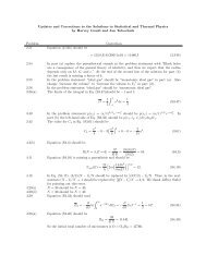
Figure 8<br />
ψ i<br />
10 CHAPTER 4. TRANSVERSE WAVES ON A STRING<br />
the case of reflecti<strong>on</strong> above, although the ψi functi<strong>on</strong> isn’t applicable for positive x, we can<br />
mathematically imagine ψi still proceeding to the right. The situati<strong>on</strong> is shown in Fig. 7. As<br />
above, let’s say that v2 = 3v1, which means that the 2v2/(v2 + v1) factor equals 3/2. Note<br />
that in any case, this factor lies between 0 and 2. We’ll talk about the various possibilities<br />
below.<br />
Figure 7<br />
ψ t<br />
v 2<br />
not really<br />
there<br />
(v2 = 3v1)<br />
ψ i<br />
v 1<br />
x = 0<br />
ψ i<br />
actual<br />
<str<strong>on</strong>g>waves</str<strong>on</strong>g><br />
(ψ r not shown)<br />
In the first picture in Fig. 7, the incident wave is moving in from the left, and the<br />
transmitted wave is also moving in from the left. The transmitted wave doesn’t actually<br />
exist to the left of x = 0, of course, but it’s c<strong>on</strong>venient to imagine it coming in as shown.<br />
With v2 = 3v1, the transmitted wave is 3/2 as tall and 3 times as wide as the incident wave.<br />
In the sec<strong>on</strong>d picture in Fig. 7, the incident wave has passed the origin and c<strong>on</strong>tinues<br />
moving to the right, where it doesn’t actually exist. But the transmitted wave is now located<br />
<strong>on</strong> the right side of the origin and moves to the right. This is the real piece of the wave.<br />
For simplicity, we haven’t shown the reflected ψr wave in these pictures, but it’s technically<br />
also there.<br />
In between the two times shown in Fig. 7, things are easier to deal with than in the<br />
reflected case, because we d<strong>on</strong>’t need to worry about taking the sum of two <str<strong>on</strong>g>waves</str<strong>on</strong>g>. The<br />
transmitted wave c<strong>on</strong>sists <strong>on</strong>ly of ψt. We d<strong>on</strong>’t have to add <strong>on</strong> ψi as we did in the reflected<br />
case. In short, ψL equals ψi + ψr, whereas ψR simply equals ψt. Equivalently, ψi and ψr<br />
have physical meaning <strong>on</strong>ly to the left of x = 0, whereas ψt has physical meaning <strong>on</strong>ly to<br />
the right of x = 0.<br />
Fig. 8 shows some successive snapshots that result from the same square wave we c<strong>on</strong>-<br />
sidered in Fig. 6. The bold-line wave indicates the actual wave that exists to the right of<br />
x = 0. We haven’t drawn the reflected wave to the left of x = 0. We’ve squashed the x<br />
axis relative to Fig. 6, to make a larger regi<strong>on</strong> viewable. These snapshots are a bit boring<br />
compared with those in Fig. 6, because there is no need to add any <str<strong>on</strong>g>waves</str<strong>on</strong>g>. As far as ψt<br />
is c<strong>on</strong>cerned <strong>on</strong> the right side of x = 0, what you see is what you get. The entire wave<br />
(<strong>on</strong> both sides of x = 0) is obtained by juxtaposing the bold <str<strong>on</strong>g>waves</str<strong>on</strong>g> in Figs. 6 and 8, after<br />
expanding Fig. 8 in the horiz<strong>on</strong>tal directi<strong>on</strong> to make the unit sizes the same (so that the ψi<br />
<str<strong>on</strong>g>waves</str<strong>on</strong>g> have the same width).<br />
ψ t