Transverse waves on a string - People.fas.harvard.edu

-
-
1.0
0.5
0.0
0.5
1.0
Ae -κx cos(ωt-Kx+φ)
10 20 30 40 50 60
Figure 26
Ae -κx
28 CHAPTER 4. TRANSVERSE WAVES ON A STRING
we’re looking at a wave that travels rightward from x = 0), then κ is positive. Plugging
k ≡ K − iκ into Eq. (73) gives
ψ(x, t) = De −κx e i(ωt−Kx) . (76)
A similar solution exists with the opposite sign in the imaginary exponent (but the e −κx
stays the same). The sum of these two solutions gives the actual physical (real) solution,
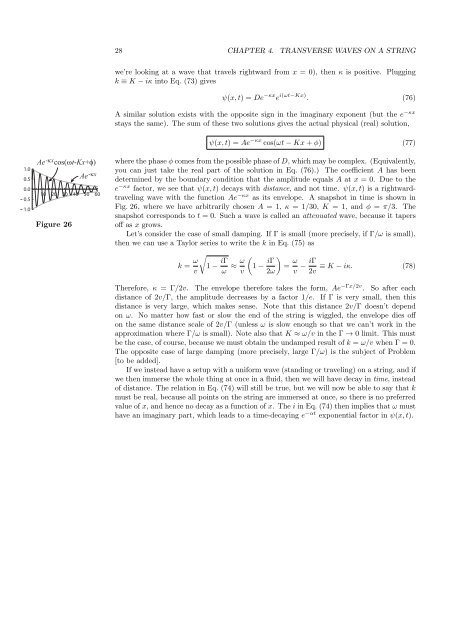
ψ(x, t) = Ae −κx cos(ωt − Kx + φ) (77)
where the phase φ comes from the possible phase of D, which may be complex. (Equivalently,
you can just take the real part of the solution in Eq. (76).) The coefficient A has been
determined by the boundary condition that the amplitude equals A at x = 0. Due to the
e −κx factor, we see that ψ(x, t) decays with distance, and not time. ψ(x, t) is a rightwardtraveling
wave with the function Ae −κx as its envelope. A snapshot in time is shown in
Fig. 26, where we have arbitrarily chosen A = 1, κ = 1/30, K = 1, and φ = π/3. The
snapshot corresponds to t = 0. Such a wave is called an attenuated wave, because it tapers
off as x grows.
Let’s consider the case of small damping. If Γ is small (more precisely, if Γ/ω is small),
then we can use a Taylor series to write the k in Eq. (75) as
k = ω
1 −
v
iΓ
ω
≈ 1 −
ω v
iΓ
=
2ω
ω iΓ
− ≡ K − iκ. (78)
v 2v
Therefore, κ = Γ/2v. The envelope therefore takes the form, Ae −Γx/2v . So after each
distance of 2v/Γ, the amplitude decreases by a factor 1/e. If Γ is very small, then this
distance is very large, which makes sense. Note that this distance 2v/Γ doesn’t depend
on ω. No matter how fast or slow the end of the string is wiggled, the envelope dies off
on the same distance scale of 2v/Γ (unless ω is slow enough so that we can’t work in the
approximation where Γ/ω is small). Note also that K ≈ ω/v in the Γ → 0 limit. This must
be the case, of course, because we must obtain the undamped result of k = ω/v when Γ = 0.
The opposite case of large damping (more precisely, large Γ/ω) is the subject of Problem
[to be added].
If we instead have a setup with a uniform wave (standing or traveling) on a string, and if
we then immerse the whole thing at once in a fluid, then we will have decay in time, instead
of distance. The relation in Eq. (74) will still be true, but we will now be able to say that k
must be real, because all points on the string are immersed at once, so there is no preferred
value of x, and hence no decay as a function of x. The i in Eq. (74) then implies that ω must
have an imaginary part, which leads to a time-decaying e −αt exponential factor in ψ(x, t).