Proc. 'ESA Living Planet Symposium', Bergen, Norway 28 June – 2 ...

_________________________________________________
Proc. ‘ESA Living Planet Symposium’, Bergen, Norway
28 June – 2 July 2010 (ESA SP-686, December 2010)

Vzz(E)
3000
2500
2000
1500
1000
500
0
measured
computed
measured-computed
-500
00:00:00 02:00:00 04:00:00 06:00:00 08:00:00 10:00:00 11:59:59 14:00:00
time on 01-Nov-2009
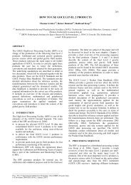
Figure 1. Measured gravity field gradients of GOCE for
a half day and computed gravity field gradients from a
gravity field model and the difference as a first estimation
for the gradiometer noise
Vzz(E)
1.5
1
0.5
0
-0.5
measured - GRS80 (mean reduced)
computed - GRS80 (mean reduced)
measured-computed (mean reduced)
-1
00:00:00 01:00:00 02:00:00
time on 01-Nov-2009
03:00:00 04:00:00
Figure 2. Reduced (mean and GRS80) measured gravity
field gradients of GOCE for 3 hours and computed
gravity field gradients from a gravity field model and the
difference as a first estimation for the gradiometer noise
gravity field model (GO CONS EGM TIM 2I, cf. [12]),
are shown as timeseries. The differences of both timeseries,
measured gradients minus computed gradients, are
an estimation for the gradiometer noise 1 . The timeseries
shown in Fig. 1 is dominated by the large bias in the measured
gradients. Thus, in the displayed scale, the noise
looks only like a bias. Removing the GRS80 signal from
the measured and computed gradients and a mean value
from the observations gives a better impression of the detailed
structure of the measurement noise (cf. Fig. 2).
The resulting (i.e. mean reduced) noise estimation shows
now an additional drift 2 and some long wavelength oscillations,
indicating the strong autocorrelations. The resulting
noise is definitely non-white.
1 Note that the three diagonal components Vxx, Vyy and Vzz show
very similar behavior, but only the Vzz component is shown here.
2 The drift is hard to recognize in this short timeseries of about 3
hours.
Figure 3. Mean reduced noise estimation of the gradiometer
for the Vzz component in the spatial domain.
It is dominated by a one per revolution error
Error [mE/sqrt(Hz)]
10 4
10 3
10 2
10 1
10 0
10 −4
10 −3
PSD
10 −2
Frequency [Hz]
GOCE noise PSD V zz
Gradient signal PSD V zz
GOCE measurement PSD V zz
Figure 4. Error spectrum of the gradiometer noise for
the Vzz component, the gradient signal and the measured
gravity gradients
To get an idea of the spatial behavior, Fig. 3 shows the
mean-reduced gradiometer noise in the GRF for ascending
and descending tracks. It is dominated by a one per
revolution oscillating error. These characteristics can be
shown in the spectral domain of the timeseries very well.
The power spectral density (i.e. the Fourier transform of
the autocorrelation function) from the noise timeseries,
the Earth’s gravity gradient signal (computed from a set
of spherical harmonics of a final GOCE solution) and the
measurements themselves for the Vzz can be seen in Fig.
4 3 .
Analyzing Fig. 4, several characteristics of the estimated
gradiometer noise can be observed. Within the socalled
measurement bandwidth (MBW, between 0.005
and 0.1 Hz), the error spectrum is more or less flat, in
this bandwidth the noise is nearly white. Ranging from
0 to 0.005Hz the error spectrum is mainly characterized
by an inverse proportional dependence (approx. 1/f) and
a large number of sharp peaks. This reflects exactly the
expected behavior, which could be seen in different case
studies before launch of the satellite (e.g. [16]).
3 Note that all other components (Vxx and Vyy) have similar characteristics,
but the level of the noise differs in the MBW (i.e. ≈
8mE/ √ Hz for Vxx, 7mE/ √ Hz for Vyy and 12mE/ √ Hz for
Vzz).
10 −1

When estimating the gravity field parameters via a rigorous
least-squares adjustment, this correlation pattern
would normally have to be taken into account by including
the known (or an estimated approximation of the)
data covariance matrix (as a metric) into the normal equations.
However, due to the huge number of SGG data, this
covariance matrix cannot be stored considering a memory
requirement of more than 20 PetaByte. An effective
solution to this problem consists in a full decorrelation
(”whitening process”) of the SGG data before the evaluation
of the normal equations 4 . Such a decorrelation can
be performed effectively through an application of digital
filters to the SGG observations and the corresponding
observation equations (cf. [13], [14], [19] and [9]).
3. MODELING THE GRADIOMETER NOISE
After describing the main characteristics of the gradiometer
noise in the previous section, we will focus on the
modeling of the noise in the following subsections. As
the full variance/covariance matrix of the gradiometer
observations is even to large to be stored on supercomputers,
the idea of describing the noise characteristics
by an ARMA process was developed in [13]. The inverse
process, which can be seen as a digital filter, can be
used to decorrelate the observations and corresponding
functional model. The transformed observation equations
have white noise and are uncorrelated (e.g. [8], p. 154f.),
such that the least squares adjustment in the gravity field
determination can be performed with a covariance matrix
equaling the identity matrix.
To get a better understanding of the coherence between
digital filters and variance/covariance matrices, in [14] it
is shown how a digital ARMA filter can be transformed
to a variance/covariance matrix. To interpret the following
figures of the noise and the estimated decorrelation
filters in the spectral domain, remind that a filtering in
the time domain is an element by element multiplication
in the spectral domain. Thus, we need to find a filter with
a spectral behavior inverse to the spectral noise behavior
seen in Fig. 4. If we are able to find such a filter, the multiplication
in the spectral domain would follow a curve
constantly equaling 1.0, which is the PSD of white noise.
Thus, we try to estimate a filter, which inverse PSD approximates
the estimated PSD of the noise (cf. Fig. 4)
as good as possible, under the additional condition that it
can be described by as less as possible coefficients. Methods
to estimate such filters of different complexity as cascades
of ARMA filters are explained in detail in e.g. [14]
and [19]. Within this contribution, we will not focus on
the technical side, but show the influence of filters modeling
the noise with different complexities.
4 This means a complete decorrelation, as e.g. described in [8], p.
154f. of the observations and the functional model.
Error [mE/sqrt(Hz)]
10 4
10 3
10 2
10 1
10 0
10 −4
10 −1
10 −3
zz
10 −2
Frequency [Hz]
GOCE noise PSD
filter 9295
Figure 6. Noise PSD ans PSD for the inverse filter 9295
(MBW band-pass filter). The figure is only shown for th
Vzz component. The other diagonal components have all
very similar characteristics.
3.1. Concentrating on the measurement bandwidth
A first idea could be, to apply a filter, which focuses on
the MBW, where the noise spectrum is flat and thus already
close to white noise. Thus, a band-pass filter could
be used to filter the signal and the functional model to the
measurement bandwidth. An estimated (inverse) bandpass
filter can be seen in Fig. 6, designed for the gradiometer’s
MBW, indicated by the black dashed lines.
Applying this filter to the observation equations of the
gradiometer measurements in the gravity field determination
from gradiometer only observations, all information
below the MBW is omitted (long wavelength noise
but also parts of the signal). Thus, the high quality data
within the MBW are processed, but the information outside
the MBW is ignored in the estimation process.
Gravity field determination with such a kind of filter is
possible – but has some disadvantages, as shown in the
following. A gradiometer only gravity field solution computed
with this filter is shown in terms coefficient differences
to the 7 years based GRACE only model ITG-
Grace2010s (cf. [10]) to the maximal resolution of the
GRACE field which is d/o 180. Fig. 5(a) shows that
the coefficient errors (i.e. coefficient differences to the
GRACE model) to d/o 50 are very large. Note that to d/o
120 the GRACE model can be seen as a kind of reference
solution, as GRACE is more sensitive to the lower
degrees then the GOCE solution. The error per degree
decreases from d/o 50 to d/o 100 but is still very large to
d/o 100 for the sectorial coefficients 5 .
These quality characteristics of the sectorial and near sectorial
coefficients are reflected by the estimated spherical
harmonic coefficient accuracies shown in Fig. 5(b). The
standard deviations show, that the sectorial coefficients to
degree 100 are bad determined as indicated in the coefficient
differences to the ITG-Grace2010s model. The co-
5 It should be mentioned in this context that intentionally a very moderate
band-pass filter was chosen, where the noise reduction in the stopband
is only in the magnitude of 60 dB this avoids a singularity of the
SGG gravity field solution.
10 −1

degree
0
60
120
180
180
120
sin
60
0 60 120 180
cos
−8
−9
−10
−11
−12
(a) Coefficient differences of SGG only solution computed with the filter
9295 compared to ITG-Grace2010s.
degree
0
60
120
180
180
120
sin
60
0 60 120 180
(c) Coefficient differences of a SGG only solution computed with the filter
1000 compared to ITG-Grace2010s.
degree
0
60
120
180
180
120
sin
60
cos
0 60 120 180
(e) Coefficient differences of a SGG only solution computed with the filter
9024 compared to ITG-Grace2010s.
degree
0
60
120
180
180
120
sin
60
cos
0 60 120 180
(g) Coefficient differences of a SGG only solution computed with the filter
9025 compared to ITG-Grace2010s.
cos
−8
−9
−10
−11
−12
−8
−9
−10
−11
−12
−8
−9
−10
−11
−12
log 10
log 10
log 10
log 10
degree
0
60
120
180
180
120
sin
60
0 60 120 180
(b) Estimated formal coefficient accuracies of SGG only solution computed
with the filter 9295.
degree
0
60
120
180
180
120
sin
60
cos
0 60 120 180
(d) Estimated formal coefficient accuracies of a SGG only solution computed
with the filter 1000.
degree
0
60
120
180
180
120
sin
60
cos
0 60 120 180
(f) Estimated formal coefficient accuracies of a SGG only solution computed
with the filter 9024.
degree
0
60
120
180
180
120
sin
60
cos
0 60 120 180
(h) Estimated formal coefficient accuracies of a SGG only solution computed
with the filter 9025.
Figure 5. Coefficient statistics for all four presented SGG solutions with the four different filters. The shown statistics are
difference to the ITG-Grace2010s model (left column), estimated formal coefficient standard deviations (right column).
cos
−8
−9
−10
−11
−12
−8
−9
−10
−11
−12
−8
−9
−10
−11
−12
−8
−9
−10
−11
−12
log 10
log 10
log 10
log 10

Error [mE/sqrt(Hz)]
10 4
10 3
10 2
10 1
10 0
10 −4
10 −1
10 −3
zz
10 −2
Frequency [Hz]
GOCE noise PSD
filter 1000
Figure 7. Noise PSD ans PSD for the inverse filter 1000
(differentiation filter). The figure is only shown for th Vzz
component. The other components have all very similar
characteristics.
efficient differences compared to ITG-Grace2010s in the
lower degrees show an agreement to the estimated variances.
In the degrees 80 to 150, the differences to the
GRACE model are well described by the corresponding
GOCE accuracies. The displayed high degrees are dominated
by the GRACE error, the GOCE variances show
that GOCE performs better starting from degree 150. The
high degrees 180-220, are not shown, as they cannot be
compared to the lower degree GRACE model.
Using a band-pass filter as shown in Fig. 6 produces a
useful gradiometer only gravity field and realistic estimates
for the coefficient variances, but has the disadvantage
that gradiometer information in the lower frequencies
is ignored and that effects the sectorial coefficients to
degree 100 6 . This can be more or less compensated when
combining the gradiometer observation with the GPS observations
from GPS tracking (SST).
3.2. Modeling the long wavelength errors
As the band-pass filter produces systematic errors for
the sectorial coefficients, a further idea of the filter design
would be to model the noise characteristics for the
low frequencies. Thus a filter could be estimated, which
down-weights the lower frequencies but keeps all information
starting from the MBW. This means, we do not filter
out the long wavelengths completely, but model their
the poor quality in the adjustment. A very simple filter
could be a differentiation filter (ID 1000) as shown in
Fig. 7. These filter can be used to decorrelate the observed
gradients and start the gravity field determination
as a spherical harmonic series.
A comparison of a solution using this filter as stochastic
information for the gradients to GRACE is shown in Fig.
5(c). Obviously the lower degree coefficient differences
6 Note that the better the band-pass filter approximates an ideal bandpass
filter the higher the degrees where the sectorial coefficients are
estimated bad. The effect of ill-defined sectorial coefficients would be
intensified with a higher noise reduction in the stop-band.
10 −1
Error [mE/sqrt(Hz)]
10 4
10 3
10 2
10 1
10 0
10 −4
10 −1
10 −3
zz
10 −2
Frequency [Hz]
GOCE noise PSD
filter 9024
Figure 8. Noise PSD ans PSD for the inverse filter 9024.
The figure is only shown for th Vzz component. The other
components have all very similar characteristics
to GRACE (to d/o 80) are smaller than for the band-pass
filter solution. The sectorial coefficients are determined
well starting from d/o 20. It can be seen clearly in the
variances, that the information outside the MBW contains
information especially for the sectorial coefficients. The
estimated accuracies in Fig. 5(d) show the better stability
of the sectorial coefficients. The quality of the solution
gets better, but the estimated accuracies have a wrong
shape for the higher degrees (d/o 120+). The formal errors
for the low orders of higher degrees are estimated too
optimistic. This results from the incomplete modeling of
the filter of the MBW frequencies. The filter introduces
a weighting in the MBW which is not correct. Using the
information of the whole spectrum seems to be a good
idea, but a kind of mixture between the band-pass filter
model and this filter model needs to be found to combine
the advantages of both models.
3.3. Simple modeling of the complete spectrum
Combining simple filters to a consecutive filter series (so
call filter cascades) allow for the design of more complex
filters. A filter should be designed which approximates
the complete noise spectrum and not only parts of it, as
did by the models before. Thus, in Fig. 8 a filter was
designed modeling long wavelength errors as well as the
MBW as good as possible. The smallest number of filter
coefficients possible was used to keep the model simple.
The filter constitutes two cascades, one modeling the long
wavelength part (similar to filter 1000) and a second one,
an ARMA filter of a higher order modeling the high pass
filtered rest correlations in the context of a least squares
fit. Connecting both filter parts, the PSD plot in Fig. 8
shows the approximation of the noise. This filter with
ID 9024 needs only 50 AR and 50 MA coefficients per
gradiometer component to describe the whole noise behavior.
Additionally it has only a short warmup (2000
positions will be lost as filter initialization). The resulting
gravity field solution combines the advantages of the
band-pass filter solution and the difference filter solution.
The solution is at least as good as the difference
10 −1

Error [mE/sqrt(Hz)]
10 4
10 3
10 2
10 1
10 0
10 −4
10 −1
10 −3
zz
10 −2
Frequency [Hz]
GOCE noise PSD
filter 9025
Figure 9. Noise PSD ans PSD for the inverse filter 1000.
The figure is only shown for th Vzz component. The other
components have all very similar characteristics
filter solution in all degrees (cf, Fig. 5(e)) as it shows
mainly the same difference pattern compared to ITG-
Grace2010s. The benefit of this modeling is visible in
the estimated spherical harmonic coefficient standard deviations.
The higher degree error is modeled very well
by the estimated formal spherical harmonic coefficient errors
(cf. Fig. 5(f)), the shape of the errors shows a good
agreement for the errors compared to GRACE up to degree
150.
3.4. Complex modeling of the complete spectrum
Analyzing the filter with the ID 9024 (cf. Fig. 8), it can
be seen that the n per revolution peaks in the spectrum
are not modeled individually. Instead, this pattern is approximated
simple (it seems to be linear in the double
logarithmic plot). To improve the filter modeling, additional
cascades could be added constituting special Notch
filters (e.g. [19]) eliminating special frequencies from the
signal. Thus, the filter is extended by several new filter
cascades, each eliminating one of the sharp peaks in the
spectrum. This filter (ID 9025) can be seen in Fig. 9.
It consists of 20 cascades with about 100 AR and 100
MA coefficients. The notch filter cascades, realized as
ARMA(2,2) filters, are responsible for a filter warmup of
200000 positions 7 . Computing a gradiometer-only gravity
field solution with this kind of filter, we see no improvement
in the solution (cf. Fig 5(g)) compared to the
former model, but an improvement in the estimated variances
is evident.
Comparing the coefficients estimated with filter 9024 and
9025 to the ITG-Grace2010s model coefficients, larger
errors can be seen in the lower degree coefficients with
the orders 16, 32, 48, 64. These are ill-defined coefficients
due to the n per revolution error. Modeling these
error peaks within the complex filter, these bad determined
coefficients are indicated in the estimated coefficient
accuracies (cf. Fig 5(h)). Thus, modeling the filter
as complex as possible, we map the error structure
7 This means, using this filter in the gravity field determination,
200000 observations are thrown away during the filter initialization.
10 −1
(b) Highpass filter
(a) unfiltered SGG errors (c) Highpass filtered errors
(g) fully filtered errors
(f) ARMA filter
(d) Notch filters
(e) Notch filtered errors
Figure 10. Effect of the different filter cascades in the
decorrelation process illustrated in the spectral domain
of the GOCE gradiometer as good as possible to the coefficient
accuracies of the estimated spherical harmonic
expansion. Thus, we achieve a high quality and realistic
formal error variance/covariance matrix. The effect of all
cascades of this complex filter is summarized within Fig.
10.
4. COMBINATION WITH GPS OBSERVATIONS
Within SPF6000 the Tuning-machine is used to estimate
a decorrelation filter for the gradiometer observation for
the gravity field determination using the time wise approach
amongst others. As the first GOCE gravity field
model is only based on 71 days of gradiometer observations,
we decided to use the simple filter 9024 for the final
GO CONS EGM TIM 2I solution. The simple filter
model was preferred in order to keep the filter warmup
short within the first short data period (2000 instead of
200000). But these complex filters will be used in future
gravity field solutions, when the data period is longer and
thus the coverage is better. It was shown above, that the
filters are globally similar, but filter 9024 does not map
the ill-defined orders to the variance/covariance matrix.
At first, this seems to be uncritical, as this ill-defined orders
are mainly in the low degrees, which are determined
mainly by the GPS observations within the final solution.
But, a look into the details shows that inconsistencies between
the data and the covariance modeling stresses the
combined solution. Modeling of the ill-defined orders in
the gradiometer covariances yields to a higher weight of
the GPS observations for this coefficients. This yields to
a better final solution after combining gradiometer and
GPS observations as the relative weights are more realistic.
Fig. 11 shows a combined GOCE solution, a gradiometer
only solution (SGG) and a solution determined by GPS
tracking (SST) using the energy balance approach (e.g.
[3]). Fig. 11 shows an improvement of the combined so-

degree variance
10 0
10 −1
10 −2
10 −3
10 −4
EIGEN5C SST
SGG SST+SGG
0 50 100 150 200
sh degree
Figure 11. Degree variances estimated using coefficient
differences to the EIGEN5C model computed without the
near zonal coefficients to exclude the effect of the polar
gap. Shown is a gradiometer only solution (SGG), a solution
only computed from the GPS tracking (SST) and the
combined one, compared to the Signal of the EIGEN5C.
lution from d/o 20 combining the SST only model with
the SGG observations. This shows, that a long wavelength
error modeling of the gradiometer noise is essential,
if the best solution based on only GOCE observations
should be determined.
Comparing the final GO CONS EGM TIM 2I model to
independently determined gravity field models, the consistence
of the models in terms of degree variances can be
shown clearly. Fig. 12 shows the final SPF6000 solution
compared to the ITG-Grace2010s solution. Especially in
the lower degrees, the 7 year based GRACE model is better
than the GOCE only model based on just 71 days. The
degree variances estimated from coefficient differences
show a very good agreement with the estimated GOCE
model accuracies to d/o 120. Starting from d/o 120 the
GOCE solution becomes more accurate than the GRACE
solution. For the very high degrees 150 - 180, where
GOCE performs better, the GRACE accuracies show a
good agreement to the difference to the GOCE model.
Fig. 13 shows the final GO CONS EGM TIM 2I solution
compared to the EIGEN5C model (c.f. [6]),
which is a high degree combination model, including
e.g. GRACE, altimetry and terrestrial data. For the
low degrees (90) the combined model performs better
than GOCE, due to the included GRACE observations.
The estimated GOCE accuracies show again a consistent
compared to the error estimated from the coefficient
differences. From degree 90 to 190, GOCE improves
the combined model, the accuracies of the combined
EIGEN5C model follow the difference curve, as
the GOCE accuracies are smaller. For the higher degrees
200+, the combined model performs better again, due to
the high frequency sensitive terrestrial data included in
the combination model.
degree variance
10 0
10 −1
10 −2
10 −3
10 −4
ITG GRACE2010S WP6000
0 50 100 150
sh degree
Figure 12. Degree variances estimated using coefficient
differences to the ITG-Grace2010s model computed
without the near zonal coefficients to exclude the effect
of the polar gap. Shown is the combined final
WP6000 (GO CONS EGM TIM 2I) solution compared
to the GRACE only model ITG-Grace2010s. The degree
variances estimated from formal errors are shown as a
dashed line.
degree variance
10 0
10 −1
10 −2
10 −3
10 −4
EIGEN5C WP6000
0 50 100 150 200
sh degree
Figure 13. Degree variances estimated using coefficient
differences to the EIGEN5C model computed
without the near zonal coefficients to exclude the effect
of the polar gap. Shown is the combined final
WP6000 (GO CONS EGM TIM 2I) solution compared
to the model EIGEN5C. The degree variances estimated
from formal errors are shown as a dashed line.
5. SUMMARY AND CONCLUSIONS
The presented tuned decorrelation filters are used within
GOCE HPF SPF6000, determining a GOCE only gravity
field using the so-called time-wise approach. We showed
that we spent a huge numerical effort to determine digital
filters, that can be used to decorrelate the GOCE gradient
observations for the purpose of gravity field determination.
We showed that a modeling of the complete
error spectrum is essential to compute the best possible
gravity field from GOCE observations. In addition, the
full variance/covariance matrix will be distributed with
the final solution (cf. [12]). Compared to independent

models (ITG-Grace2010s and EIGEN5C) the estimated
formal accuracies show a consistent model. The provided
variance/covariance matrix is of a very high quality,
as it is modeled straight forward throughout all computation
steps of GOCE only gravity field determination
steps. As no external information is included in the solution,
the solution and the variance/covariance matrix are
thus self-consistent. We recommend to use the full variance/covariance
matrix in as many applications as possible,
where the GOCE model is used. As can be seen in
comparison to independent models, the provided covariance
matrix reflects the true error characteristics of the
GOCE gravity field solution. With the coefficients and
the full variance/covariance matrix, indirectly the full set
of normal equations are available, which allows for the
use in combination models (e.g. with GRACE, altimetry
or terrestrial data).
ACKNOWLEDGMENTS
Parts of this work were financially supported by the
BMBF Geotechnologien program REAL-GOCE and the
ESA GOCE HPF contract No. 18308/04/NL/MM. The
computations were performed on the JUROPA supercomputer
in Jülich. The computing time was granted by John
von Neumann Institute for Computing (project HBN15).
REFERENCES
[1] H. Alkhatib. On Monte Carlo methods with applications
to the current satellite gravity missions.
PhD thesis, Institute of Geodesy and Geoinformation,
University of Bonn, Bonn, 2007.
[2] H. Alkhatib and W.-D. Schuh. Integration of the
Monte Carlo covariance estimation strategy into
tailored solution procedures for large-scaled least
squares problems. Journal of Geodesy, 70:53–66,
2007.
[3] T. Badura. Gravity Field Analysis from Satellite
Orbit Information applying the Energy Integral Approach.
PhD thesis, TU Graz, Graz, 2006.
[4] C. Boxhammer. Effiziente numerische Verfahren
zur sphärischen harmonischen Analyse von Satellitendaten.
PhD thesis, Institute of Geodesy and
Geoinformation, University of Bonn, Bonn, 2006.
[5] J.M. Brockmann, B. Kargoll, I. Krasbutter, W.-
D. Schuh, and M. Wermuth. GOCE data analysis:
From calibrated measurements to the global earth
gravity field. In N.N., editor, Observation of the
Earth System from Space, accepted. Springer, 2009.
[6] C. Foerste, F. Flechtner, R. Schmidt, R. Stubenvoll,
M. Rothacher, J. Kusche, K.-H. Neumayer,
R. Biancale, J.-M. Lemoine, F. Barthelmes, S. Bruinsma,
R. Koenig, and U. Meyer. EIGEN-GL05C
- A new global combined high-resolution GRACEbased
gravity field model of the GFZ-GRGS cooperation.
In Geophysical Research Abstracts,
volume 10 of General Assembly European Geosciences
Union, Vienna, 2008.
[7] M. Hestenes and E. Stiefel. Methods of conjugate
gradients for solving linear systems. Journal of Research
of the National Bureau of Standards, 49 (6),
Research Paper 2379, 1952.
[8] K.R. Koch. Parameter Estimation and Hypothesis
Testing in Linear Models. Springer
Berlin/Heidelberg, 2 edition, 1999.
[9] I. Krasbutter. Dekorrelation und Daten-TÜV der
GOCE-Residuen. Diploma thesis, Universität
Bonn, Bonn, 2009.
[10] T Mayer-Gürr, E. Kurtenbach, and A. Eicker.
ITG-Grace2010s. http://www.igg.unibonn.de/apmg/index.php?id=itg-grace2010,
2010.
[11] R. Pail, B. Metzler, B. Lackner, T. Preimesberger,
E. Hck, W.-D. Schuh, H. Alkathib, C. Boxhammer,
C. Siemes, and M. Wermuth. GOCE gravity field
analysis in the framework of HPF: operational software
system and simulation results. In 3 rd GOCE
user workshop, Frascati, 2006. ESA.
[12] R. Pail, H. Goiginger, R. Mayrhofer, W.-D. Schuh,
J. M. Brockmann, I. Krasbutter, E. Hck, and
T. Fecher. GOCE gracity field model derived from
orbit and gradiometry data applying the time-wise
method. In Proceedings of the ESA Living Planet
Symposium, Bergen, 28 June 2 July 2010. ESA.
[13] W.D. Schuh. SST/SGG tailored numerical solution
strategies. Technical report, ESA-Project
CIGAR III / Phase 2, WP 221, Final-Report, Part
2, 1995.
[14] W.-D. Schuh. Tailored Numerical Solution Strategies
for the Global Determination of the Earth’s
Gravity Field, volume 81 of Mitteilungen der
geodätischen Institute der Technischen Universität
Graz. TU Graz, Graz, 1996.
[15] W.-D. Schuh. The processing of band-limited measurements;
filtering techniques in the least squares
context and in the presence of data gaps. In G. Beutler,
M.R. Drinkwater, R. Rummel, and R. von
Steiger, editors, Earth Gravity Field from Space -
From Sensors to Earth Sciences, volume 108, pages
67–78. Space Science Reviews, 2003. ISSI Workshop,
Bern (March 11-15,2002).
[16] W.-D. Schuh, C. Boxhammer, and C. Siemes. Correlations,
variances, covariances — from GOCE
signals to GOCE products. In 3 rd GOCE user workshop,
Frascati, 2006. ESA.
[17] W.-D. Schuh, J.M. Brockmann, B. Kargoll, and
I. Krasbutter. Adaptive Optimization of GOCE
Gravity Field Modeling. In G. Münster et. al.,
eds, NIC Symposium 2010, IAS Series, 3:313–320,
Jülich, 2010.
[18] H.R. Schwarz. Die Methode der konjugierten Gradienten
in der Ausgleichsrechnung. ZfV, 95:130–
140, 1970.
[19] C. Siemes. Digital Filtering Algorithms for Decorrelation
within Large Least Squares Problems. PhD
thesis, Institute of Geodesy and Geoinformation,
University of Bonn, Bonn, 2008.