A4 - Faculty.jacobs-university.de

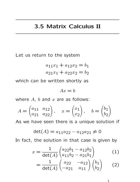
3.5 Matrix Calculus II
Let us return to the system
a11x1 + a12x2 = b1
a21x1 + a22x2 = b2
which can be written shortly as
Ax = b
where A, b and x are as follows:
A =
a11
a12
a21 a22
, x =
x1
x2
, b =
b1
b2
As we have seen there is a unique solution if
det(A) = a11a22 − a12a21 = 0
In fact, the solution in that case is given by
x =
=
1
det(A)
1
det(A)
a22b1 − a12b2
a11b2 − a21b1
a22 −a12 b1
−a21 a11 b2
1
(1)
(2)

3.5 Matrix Calculus II
Now it is tempting to multiply the matrix
equation Ax = b by a matrix A −1 such that
x = A −1 Ax = A −1 b
If we compare this with (1) and (2) then it
follows that
A −1 =
1
det(A)
a22 −a12
−a21 a11
We have A −1 A = AA −1 = E, that is, A has
an inverse matrix. For det(A) = 0 there
does not exist an inverse matrix for A. The
definition of an invertible matrix is as follows:
Definition (Non-singular matrix). A square
matrix A ∈ Mn is called non-singular or invertible
if there exists a matrix B ∈ Mn such
that
AB = E = BA
Any matrix B with the above property is
called an inverse of A. If A does not have
an inverse, A is called singular.
2

3.5 Matrix Calculus II
Theorem (Inverses are unique). If A has
inverses B and C, then B = C.
Proof. If B and C are inverses of A then
AB = E = BA and AC = E = CA. It follows
B = BE = B(AC) = (BA)C = EC = C
Notation: If A has an inverse, it is denoted
by A −1 . So AA −1 = A −1 A = E.
Example: A =
1 2
4 8
is singular. For sup-
pose B =
a
c
b
d
is an inverse of A. Then
AB = E implies the inconsistent system
1 = a + 2c
0 = 4a + 8c
3

3.5 Matrix Calculus II
Theorem (Unique solution of systems of
linear equations). If the coefficient matrix A
of a system of n equations in n unknowns is
non-singular, then the system Ax = b has the
unique solution x = A −1 b.
Theorem. Let A be a square matrix. If A
is non-singular, then the homogeneous system
Ax = 0 has only the trivial solution
x = 0. Equivalently, if the homogeneous system
Ax = 0 has a non-trivial solution, then A
is singular.
Example: Consider the system given by
⎛
⎜
⎝
1 2 3
4 5 6
7 8 9
⎞ ⎛ ⎞
x1
⎟ ⎜ ⎟
⎠ ⎝x2
x3
⎠ =
If we apply the Gauß-Jordan algorithm we obtain
the equivalent equation
⎛
⎜
⎝
1 0 −1
0 1 2
0 0 0
⎞ ⎛ ⎞
x1
⎟ ⎜ ⎟
⎠ ⎝x2
x3
⎠ =
⎛
⎜
⎝
0
0
0
⎛
⎜
⎝
⎞
⎟
⎠
0
0
0
⎞
⎟
⎠
4

3.5 Matrix Calculus II
We easily see a non-trivial solution
x t = (1, −2, 1)
and hence the matrix is singular.
Theorem. A square matrix A is non-singular
if and only if its reduced row-echelon form is
non-singular.
As soon as there is a zero row in A, the matrix
will be singular.
Corollary. Suppose that A, B ∈ Mn such that
AB = E. Then also BA = E.
Proof. Let AB = E and assume Bx = 0.
Then A(Bx) = A0 = 0, so that x = Ex =
(AB)x = 0. Hence B is non-singular by the
theorem. Then from AB = E we deduce
A = (AB)B −1 = EB −1 = B −1
and BA = BB −1 = E.
Theorem. If A and B are non-singular matrices
in Mn then
(AB) −1 = B −1 A −1
5

3.5 Matrix Calculus II
Recall that also (AB) t = B t A t for matrices
A, B. There are three important classes of
matrices that can be defined concisely in
terms of the transpose operation.
Definition (Symmetric matrix). A square
matrix A is called symmetric if At = A. In
other words, A = (aij) such that aij = aji for
all i, j. Hence
a b
b d
is a general 2 × 2 symmetric matrix.
Definition (Skew-symmetric matrix). A
square matrix A is called skew-symmetric if
A t = −A. In other words, A = (aij) such that
aij = −aji for all i, j. Hence
0 b
−b 0
is a general 2 × 2 skew-symmetric matrix.
6

3.5 Matrix Calculus II
Definition (Orthogonal matrix). A square
matrix A is called orthogonal if A −1 = A t .
Thus A must be necessarily non-singular.
Example: Verify that the following matrix is
orthogonal:
A =
⎛
1 8
⎜9
9
⎜
⎝
−4 9
4
9 −4 9 −7 ⎞
⎟
9
⎟
⎠
8 1 4
9 9 9
We say that vectors v1, v2, . . . , vn form an orthonormal
set if the vectors are perpendicular
to each other and have lenght one, that
is,
vi · vj =
⎧
⎨
⎩
0 if i = j,
1 if i = j
Theorem. Let A be a square matrix. Then
the following are equivalent:
(a) A is orthogonal.
(b) The rows of A form an orthonormal set.
(c) The columns of A form an orthonormal
set.
7

3.5 Matrix Calculus II
When is a matrix singular ? We want to
know this for solving systems of linear equations.
The answer is given by determinants:
each square matrix A is assigned a special
scalar called the determinant of A, denoted
by det(A) or |A|, i.e.,
a11 a12 · · · a1n
a21
.
a22
.
· · ·
· · ·
a2n
.
an1 an2 · · · ann
A will be singular if and only if det(A) = 0.
For A ∈ Mn we know formulas for n = 1, 2:
|a11| = a11,
a11
a12
a21
a22
= a11a22 − a12a21
The formulas will be much more complicated
for bigger n. For n = 3 we have
a11
a12 a13
a21
a22 a23
a31
a32 a33
= a11
+ a13
a22
a32
a23
a21
− a12
a33
a31
a23
a33
a21
a31
a22
a32
8

3.5 Matrix Calculus II
or equivalently,
det(A) = a11|A11| − a12|A12| + a13|A13|
where A1j denotes the 2 × 2 matrix obtained
from A by omission of the first row and the
j-th column. A more convenient method to
compute det(A) for A ∈ M3 is the rule of
Sarrus.
Definition (Determinant of a square matrix).
The determinant det(A) of a matrix
A ∈ Mn is recursively defined by
det(A) =
n
(−1)
j=1
1+j a1j det(A1j)
where A1j is of size n−1 and is obtained from
A by omission of the first row and the j-th
column.
As n increases, the number of terms in the determinant
becomes astronomical. We have
n! terms, and Sterling’s formula says
n! ∼ √
n n
2πn
e
9

3.5 Matrix Calculus II
For n = 4 the formula for the determinant is
given by
det(A) = a11a22a33a44 − a11a22a34a43
− a11a23a32a44 + a11a23a34a42
+ a11a24a32a43 − a11a24a33a42
− a12a21a33a44 + a12a21a34a43
+ a12a23a31a44 − a12a23a34a41
− a12a24a31a43 + a12a24a33a41
+ a13a21a32a44 − a13a21a34a42
− a13a22a31a44 + a13a22a34a41
+ a13a24a31a42 − a13a24a32a41
− a14a21a32a43 + a14a21a33a42
+ a14a22a31a43 − a14a22a33a41
− a14a23a31a42 + a14a23a32a41
Theorem. For A, B ∈ Mn holds
det(E) = 1
det(A t ) = det(A)
det(AB) = det(A) det(B)
10

3.5 Matrix Calculus II
Example: Consider the system of linear
equations Ax = b with
A =
⎛
⎜
⎝
⎞
1
4
2
5
3
⎟
6 ⎠ , x =
7 9 10
⎛ ⎞
x1
⎜ ⎟
⎝x2
x3
⎠ , b =
⎛
⎜
⎝
2
8
13
We compute det(A) = −3, hence we obtain
the unique solution by x = A−1b. How do we
compute A−1 ?
We can again use the Gauß-Jordan algorithm,
this time simultaneously on the partitioned
matrix [A | E]:
⎛
⎜
⎝
⎛
⎜
⎝
1 2 3 1 0 0
4 5 6 0 1 0
7 8 10 0 0 1
1 2 3 1 0 0
0 1 2
4
3 −1 3 0
0 0 1 1 −2 1
⎞
⎟
⎠
⎞
⎟
⎠
⎛
1 0 0 −
⎜
⎝
2 3 −4 3 1
0 1 0 − 2 11
3 3
0 0 1 1 −2
−2
1
⎞
⎟
⎠
⎞
⎟
⎠
11

3.5 Matrix Calculus II
Hence we obtain
x = A −1 b =
⎛
−
⎜
⎝
2 3 −4 3 1
− 2 11
3 3
1 −2
−2
1
⎞ ⎛
⎟ ⎜
⎠ ⎝
⎞
2
⎟
8 ⎠ =
13
⎛
⎜
⎝
1
2
−1
Least square solutions of linear equations:
Suppose Ax = b represents a system of linear
equations with real coefficients which may be
inconsistent, because of the possibility of experimental
errors in determining A or b. As an
example, the following system is inconsistent:
x1 = 1
x2 = 2
x1 + x2 = 3.001
Theorem. The associated normal equation
A t Ax = A t b
is always consistent and any solution of this
system minimizes the sum
r 2 1 + · · · + r2 m
where the residuals ri are defined by ri =
ai1x1 + · · · + ainxn − bi for i = 1, . . . , m.
12
⎞
⎟
⎠

3.5 Matrix Calculus II
Example: Consider the above inconsistent
system Ax = b with
A =
⎛
⎜
⎝
⎞
1
0
0
⎟
1⎠
, x =
1 1
Then we obtain
A t A =
2 1
1 2
x1
x2
, A t b =
So the normal equations are
, b =
2x1 + x2 = 4.001
x1 + 2x2 = 5.001
which have the unique solution
⎛
⎜
⎝
4.001
5.001
x1 = 3.001
3 , x2 = 6.001
3
The solution minimizes
1
2
3.001
r 2 1 + r2 2 + r2 3 = (x1 − 1) 2 + (x2 − 2) 2
+ (x1 + x2 − 3.001) 2
13
⎞
⎟
⎠