

Dynamics of Machines - Part II - IFS.pdf
Dynamics of Machines - Part II - IFS.pdf
Dynamics of Machines - Part II - IFS.pdf

Create successful ePaper yourself
Turn your PDF publications into a flip-book with our unique Google optimized e-Paper software.
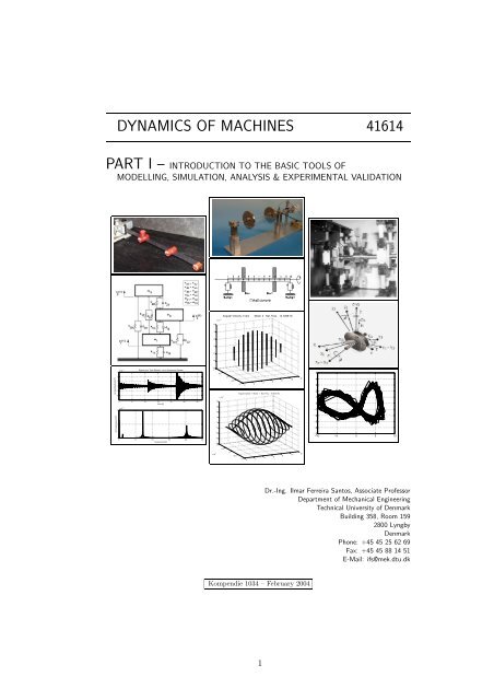
DYNAMICS OF MACHINES 41614<br />
PART I – INTRODUCTION TO THE BASIC TOOLS OF<br />
MODELLING, SIMULATION, ANALYSIS & EXPERIMENTAL VALIDATION<br />
(a) Amplitude [m/s 2 ]<br />
(b) Amplitude [m/s 2 ]<br />
x 10−4<br />
3<br />
2<br />
1<br />
0<br />
−1<br />
−2<br />
Signal (a) in Time Domain − (b) in Frequency Domain<br />
0 5 10 15<br />
time [s]<br />
20 25 30<br />
x 10−5<br />
2<br />
1<br />
0<br />
0 5 10 15 20 25<br />
frequency [Hz]<br />
6<br />
4<br />
2<br />
0<br />
−2<br />
−4<br />
−6<br />
1<br />
x 10 −4<br />
−4<br />
1<br />
x 10 −3<br />
4<br />
3<br />
2<br />
1<br />
0<br />
−1<br />
−2<br />
−3<br />
0.5<br />
x 10 −7<br />
0.5<br />
Angular Velocity: 0 rpm Mode: 2 Nat. Freq.: 14.7288 Hz<br />
0<br />
0<br />
−0.5<br />
−0.5<br />
−1 0<br />
−1 0<br />
2<br />
Angular Speed: 1 Mode: 1 Nat. Freq.: 15.6815 Hz<br />
2<br />
Kompendie 1034 – February 2004<br />
4<br />
1<br />
4<br />
6<br />
6<br />
8<br />
8<br />
10<br />
10<br />
12<br />
12<br />
5<br />
4<br />
3<br />
2<br />
1<br />
0<br />
−1<br />
−2<br />
−3<br />
−4<br />
−5<br />
−10 −5 0 5 10<br />
Dr.-Ing. Ilmar Ferreira Santos, Associate Pr<strong>of</strong>essor<br />
Department <strong>of</strong> Mechanical Engineering<br />
Technical University <strong>of</strong> Denmark<br />
Building 358, Room 159<br />
2800 Lyngby<br />
Denmark<br />
Phone: +45 45 25 62 69<br />
Fax: +45 45 88 14 51<br />
E-Mail: ifs@mek.dtu.dk
Contents<br />
1 Introduction to Dynamical Modelling <strong>of</strong> <strong>Machines</strong> and Structures and Experimental<br />
Analysis <strong>of</strong> Mechanical Vibrations based on the Human Senses 3<br />
1.1 Summary . . . . . . . . . . . . . . . . . . . . . . . . . . . . . . . . . . . . . . . . 3<br />
1.2 Description <strong>of</strong> the Test Facilities . . . . . . . . . . . . . . . . . . . . . . . . . . . 3<br />
1.3 Data <strong>of</strong> the Mechanical System . . . . . . . . . . . . . . . . . . . . . . . . . . . . 5<br />
1.4 Calculating Equivalent Stiffness Coefficients – Beam Theory . . . . . . . . . . . 5<br />
1.5 Calculating Stiffness Matrices – Beam Theory . . . . . . . . . . . . . . . . . . . 7<br />
1.6 Mechanical Systems with 1 D.O.F. . . . . . . . . . . . . . . . . . . . . . . . . . . 9<br />
1.6.1 Physical System and Mechanical Model . . . . . . . . . . . . . . . . . . . 9<br />
1.6.2 Mathematical Model . . . . . . . . . . . . . . . . . . . . . . . . . . . . . . 9<br />
1.6.3 Analytical and Numerical Solution <strong>of</strong> the Equation <strong>of</strong> Motion . . . . . . . 10<br />
1.6.4 Analytical and Numerical Solution <strong>of</strong> Equation <strong>of</strong> Motion using Matlab . 15<br />
1.6.5 Comparison between the Analytical and Numerical Solutions <strong>of</strong> Equation<br />
<strong>of</strong> Motion . . . . . . . . . . . . . . . . . . . . . . . . . . . . . . . . . . . . 16<br />
1.6.6 Homogeneous Solution or Free-Vibrations or Transient Response - Experimental<br />
Analysis . . . . . . . . . . . . . . . . . . . . . . . . . . . . . . . . 19<br />
1.6.7 Natural Frequency – ωn [rad/s] or fn [Hz] . . . . . . . . . . . . . . . . . . 19<br />
1.6.8 Damping Factor ξ or Logarithmic Decrement β . . . . . . . . . . . . . . . 19<br />
1.6.9 Forced Vibrations or Steady-State Response . . . . . . . . . . . . . . . . 24<br />
1.6.10 Resonance and Phase . . . . . . . . . . . . . . . . . . . . . . . . . . . . . 24<br />
1.6.11 Superposition <strong>of</strong> Transient and Forced Vibrations in Time Domain (Simulation)<br />
. . . . . . . . . . . . . . . . . . . . . . . . . . . . . . . . . . . . . 27<br />
1.6.12 Resonance – Experimental Analysis in Time Domain . . . . . . . . . . . . 28<br />
1.7 Mechanical Systems with 2 D.O.F. . . . . . . . . . . . . . . . . . . . . . . . . . . 31<br />
1.7.1 Physical System and Mechanical Model . . . . . . . . . . . . . . . . . . . 31<br />
1.7.2 Mathematical Model . . . . . . . . . . . . . . . . . . . . . . . . . . . . . . 31<br />
1.7.3 Analytical and Numerical Solution <strong>of</strong> System <strong>of</strong> Differential Linear Equations<br />
. . . . . . . . . . . . . . . . . . . . . . . . . . . . . . . . . . . . . . 32<br />
1.7.4 Modal Analysis using Matlab eig-function [u, w] = eig(−B, A) . . . . . . . 37<br />
1.7.5 Analytical and Numerical Solutions <strong>of</strong> Equation <strong>of</strong> Motion using Matlab . 40<br />
1.7.6 Analytical and Numerical Results <strong>of</strong> the System <strong>of</strong> Equations <strong>of</strong> Motion . 41<br />
1.7.7 Programming in Matlab – Frequency Response Analysis . . . . . . . . . . 42<br />
1.7.8 Understanding Resonances and Mode Shapes using your Eyes and Fingers 43<br />
1.7.9 Resonance – Experimental Analysis in Time Domain . . . . . . . . . . . . 48<br />
1.8 Mechanical Systems with 3 D.O.F. . . . . . . . . . . . . . . . . . . . . . . . . . . 49<br />
1.8.1 Physical System and Mechanical Model . . . . . . . . . . . . . . . . . . . 49<br />
1.8.2 Mathematical Model . . . . . . . . . . . . . . . . . . . . . . . . . . . . . . 49<br />
1.8.3 Programming in Matlab – Theoretical Parameter Studies and Experimental<br />
Validation . . . . . . . . . . . . . . . . . . . . . . . . . . . . . . . . . . 52<br />
1.8.4 Theoretical Frequency Response Function . . . . . . . . . . . . . . . . . . 55<br />
1.8.5 Experimental – Natural Frequencies . . . . . . . . . . . . . . . . . . . . . 56<br />
1.8.6 Experimental – Resonances and Mode Shapes . . . . . . . . . . . . . . . . 56<br />
1.9 Exercises . . . . . . . . . . . . . . . . . . . . . . . . . . . . . . . . . . . . . . . . 58<br />
1.10 Project 0 – Identification <strong>of</strong> Model Parameters (An Example) . . . . . . . . . . . 61<br />
1.11 Project 1 – Modal Analysis & Validation <strong>of</strong> Models . . . . . . . . . . . . . . . . . 66<br />
2
1 Introduction to Dynamical Modelling <strong>of</strong> <strong>Machines</strong> and Structures<br />
and Experimental Analysis <strong>of</strong> Mechanical Vibrations<br />
based on the Human Senses<br />
1.1 Summary<br />
The aim <strong>of</strong> this study is to show some theoretical and experimental examples to facilitate the<br />
understanding <strong>of</strong> the physical meaning <strong>of</strong> the main topics and definitions used in relation to<br />
vibrations in machines. Theoretical and experimental studies are led side-by-side, clarifying<br />
the definitions <strong>of</strong> stiffness, flexibility, natural frequency, damping factor, logarithmic decrement,<br />
resonance, phase, beating, unbalance, natural mode shape, modal node and so on. The experimental<br />
investigations are always carried out in low frequency ranges, aiming at making easy<br />
the visualization <strong>of</strong> the movements by the human eyes and the understanding <strong>of</strong> the mechanical<br />
vibrations without necessarily having to use sensors and electronic devices.<br />
1.2 Description <strong>of</strong> the Test Facilities<br />
Figures 1 and 2 show the simple elements used during the experimental investigations: a flexible<br />
beam (ruler), concentrated masses or magnets, a support, an accelerometer, a signal amplifier, a<br />
shaker and a signal analyzer. The beam or ruler already has a scale, enabling it to easily achieve<br />
the information about the position (length) where the magnets will be mounted. At each position<br />
more than one magnet can be mounted, allowing changes in the values <strong>of</strong> the concentrated<br />
masses. The masses or magnets can be easily moved and attached to different positions along<br />
the ruler, aiming at investigating changes in the natural frequencies <strong>of</strong> the magnet-ruler system<br />
(mass-spring system). The ruler is very flexible in one plane only due to the characteristic <strong>of</strong><br />
its cross-section (moment <strong>of</strong> inertia <strong>of</strong> area). The beam can easily be mounted with different<br />
boundary conditions, as free-free, clamped-free, simply supported in both ends, etc. allowing an<br />
investigation <strong>of</strong> the influence <strong>of</strong> the boundary conditions on its flexibility, and consequently on<br />
the natural frequencies <strong>of</strong> the system.<br />
Regarding rotating machines some analogies can be made between the mass-spring system presented<br />
here and a centrifugal compressor, while comparing the ruler (or flexible beam) to the<br />
flexible shaft, and the magnets (or concentrated masses) to the impellers or rigid discs. Changes<br />
in the montage <strong>of</strong> shaft into the bearings (boundary conditions) or changes in the positioning<br />
<strong>of</strong> the impellers along the shaft will lead to different critical speeds and mode shapes.<br />
As mentioned above, the mass-spring system was designed to have a very flexible behavior with<br />
very low natural frequencies. This allows the detection <strong>of</strong> natural frequencies, modes shapes<br />
and resonance using the human eyes as sensors (or sighting senses). Moreover, it is also made<br />
possible to excite the structure with human fingers, aiming at understanding the 90 degrees<br />
phase between displacement and excitation (while operating around resonance conditions) by<br />
means <strong>of</strong> tactile senses. Accelerometer, amplifier, shaker and signal analyzer are used aiming at<br />
confirming what the human senses detect.<br />
3
By understanding the topics related to mechanical vibration in low frequency ranges (high<br />
flexibility and slow motions detectable by human senses), it gets easier to understand mechanical<br />
vibration in high frequency ranges where one has faster motions with small amplitudes, just<br />
detectable by sensors and electronic devices.<br />
Figure 1: Experimental investigation <strong>of</strong> a mechanical continuous system with concentrated<br />
masses modelled as equivalent spring-mass systems with 1, 2 and 3 degrees <strong>of</strong> freedom (D.O.F.).<br />
Figure 2: Signal analyzer and shaker used for inducing and measuring mechanical vibrations<br />
while analyzing the behavior <strong>of</strong> the spring-mass systems with 1 D.O.F., 2 D.O.F. and 3 D.O.F.<br />
4
1.3 Data <strong>of</strong> the Mechanical System<br />
ρ material density <strong>of</strong> the beam 7, 800 Kg/m 3<br />
E elasticity modulus 2 × 10 11 N/m 2<br />
L total length <strong>of</strong> the beam 0.600 m<br />
b width <strong>of</strong> the beam 0.030 m<br />
h thickness 0.0012 m<br />
mi concentrated mass (i = 1, ...,6) 0.191 Kg<br />
Table 1: Data <strong>of</strong> the mass-spring system ”A”.<br />
ρ material density <strong>of</strong> the beam 7, 800 Kg/m 3<br />
E elasticity modulus 2 × 10 11 N/m 2<br />
L total length <strong>of</strong> the beam 0.300 m<br />
b width <strong>of</strong> the beam 0.025 m<br />
h thickness 0.0010 m<br />
ρ material density (steel) 7, 800 Kg/m 3<br />
mi concentrated mass (i = 1, ...,6) 0.191 Kg<br />
Table 2: Data <strong>of</strong> the mass-spring system ”B”.<br />
1.4 Calculating Equivalent Stiffness Coefficients – Beam Theory<br />
(a) (b)<br />
Figure 3: (a) Flexible beam – clamped-free boundary condition case with force applied to the end<br />
L; (b) clamped-free boundary condition case with force applied to a general position L ∗ ;<br />
By applying a vertical force F at the end <strong>of</strong> the beam as shown in figure 3(a) and using Beam<br />
Theory, one can write:<br />
EI d4y(x) = 0 (1)<br />
dx4 Integrating in X once, one has:<br />
EI d3 y(x)<br />
dx 3 = F(x) = C1 (2)<br />
5
Integrating twice in X, it gives:<br />
EI d2 y(x)<br />
dx 2 = M(x) = C1x + C2 (3)<br />
Integrating again in X, one gets the rotation angle <strong>of</strong> the beam:<br />
EI dy(x)<br />
dx<br />
x<br />
= EIΘ(x) = C1<br />
2<br />
2 + C2x + C3<br />
And finally, integrating the last time in X, one achieves the equation responsible for describing<br />
the deflexion <strong>of</strong> the beam:<br />
x<br />
EI y(x) = C1<br />
3<br />
6<br />
x<br />
+ C2<br />
2<br />
2 + C3x + C4<br />
The boundary conditions for the clamped-free beam are:<br />
•y(x = 0) = 0<br />
•Θ(x = 0) = 0<br />
•M(x = L) = 0<br />
•F(x = L) = −F (reaction)<br />
⎫<br />
⎪⎬<br />
⎪⎭<br />
After calculating the constants Ci using the boundary condition for the clamped-free beam case,<br />
one gets<br />
y(x) = − F<br />
E I<br />
dy(x)<br />
dx<br />
x 3<br />
6<br />
= Θ(x) = − F<br />
E I<br />
<br />
L x2<br />
−<br />
2<br />
x 2<br />
2<br />
<br />
− L x<br />
Using the relationship between applied force F and the induced deflexion at a given point along<br />
the beam length, x = L for instance, one gets the equivalent stiffness as:<br />
K = F<br />
y(L)<br />
= 3 EI<br />
L 3<br />
Suggestion (I): Change the beam boundary conditions, for example bi-supported at both ends,<br />
and calculate the equivalent stiffness in the new case.<br />
Suggestion (<strong>II</strong>): Change the beam boundary conditions, for example clamped-clamped at both<br />
ends, and calculate the equivalent stiffness in the new case.<br />
6<br />
(4)<br />
(5)<br />
(6)<br />
(7)<br />
(8)<br />
(9)
1.5 Calculating Stiffness Matrices – Beam Theory<br />
Two Different Lengths for Applying Forces – To facilitate the understanding <strong>of</strong> steps<br />
which will be presented, one can introduce the follow nomenclature (see figure 3(b)):<br />
• L ∗ = L1 or L ∗ = L2 – length where the force F is applied.<br />
• x = L1 or x = L2 – length where the displacement is measured.<br />
Taking into account two different points for applying the forces and measuring the displacements<br />
<strong>of</strong> the beam, one works with the following set <strong>of</strong> equations<br />
x [0, L ∗ ]<br />
and<br />
x [L ∗ , L]<br />
⎧<br />
⎪⎨<br />
⎪⎩<br />
⎧<br />
⎪⎨<br />
⎪⎩<br />
y(x) = − F<br />
E I<br />
dy(x)<br />
dx<br />
= − F<br />
E I<br />
<br />
x3 6 − L∗ x2 <br />
2<br />
<br />
x2 2 − L∗ <br />
x<br />
y(x) = y(L ∗ ) + dy(x)<br />
dx<br />
dy(x)<br />
dx<br />
= dy(x)<br />
dx<br />
<br />
<br />
x=L ∗<br />
<br />
<br />
<br />
x=L∗ · (x − L∗ )<br />
which are responsible for describing the deflection <strong>of</strong> the beam, considering the loading on<br />
different coordinates.<br />
Let us introduce an example <strong>of</strong> a system with two points <strong>of</strong> force application. Assuming in case<br />
(I) the force F is applied to the first coordinate L ∗ = L1. One can measure and/or calculate<br />
the beam deflection at the coordinates x = L1 and x = L2 through equations (10) and (11):<br />
y1 = y(L1) = F · L3 1<br />
3 · EI<br />
and<br />
y2 = y(L2) = F<br />
6EI · (2L3 1 + 3L 2 1(L2 − L1)) (13)<br />
Assuming in case (<strong>II</strong>) that the force F is applied to the second coordinate L ∗ = L2, one can<br />
measure and/or calculate the follow beam displacements at the coordinates x = L1 and x = L2<br />
through the equations (10) and (11):<br />
y1 = y(L1) = F<br />
6EI · (2L3 1 + 3L 2 1(L2 − L1)) (14)<br />
and<br />
y2 = y(L2) = F · L3 2<br />
3 · EI<br />
7<br />
(10)<br />
(11)<br />
(12)<br />
(15)
In order to calculate the stiffness matrix (k11, k12, k21, k22) <strong>of</strong> the 2 d.o.f. system,<br />
Ky = f (16)<br />
where<br />
K =<br />
k11 k12<br />
k21 k22<br />
<br />
y = { y1 y2 } T<br />
f = { f1 f2 } T<br />
one has to solve the following system <strong>of</strong> equations for case (I) and case (<strong>II</strong>):<br />
k11 k12<br />
k21 k22<br />
<br />
y1<br />
·<br />
y2<br />
<br />
=<br />
Case (I): f = { F 0 } T<br />
k11 k12<br />
k21 k22<br />
<br />
·<br />
Case (<strong>II</strong>): f = { 0 F } T<br />
k11 k12<br />
k21 k22<br />
f1<br />
f2<br />
<br />
F ·L 3 1<br />
3·EI<br />
F<br />
6EI · (2L3 1 + 3L2 1 (L2 − L1))<br />
<br />
F<br />
6EI<br />
·<br />
· (2L31 + 3L21 (L2 − L1))<br />
F ·L3 2<br />
3·EI<br />
<br />
<br />
=<br />
=<br />
F<br />
0<br />
0<br />
F<br />
It leads to a system <strong>of</strong> 4 equations, which can be written in a matrix form:<br />
⎡<br />
⎢<br />
⎣<br />
F ·L 3 1<br />
3·EI<br />
F<br />
6EI · (2L31 + 3L 2 0<br />
1(L2 − L1))<br />
0<br />
0<br />
F ·L<br />
0<br />
3 1<br />
3·EI<br />
F<br />
6EI · (2L31 + 3L 2 F<br />
6EI<br />
1(L2 − L1))<br />
· (2L31 + 3L 2 1(L2 − L1))<br />
F ·L 3 0<br />
2<br />
3·EI<br />
0<br />
0<br />
F<br />
6EI<br />
0<br />
· (2L31 + 3L 2 1(L2 − L1))<br />
F ·L 3 ⎤<br />
⎥<br />
⎦<br />
2<br />
3·EI<br />
·<br />
⎧<br />
⎪⎨<br />
·<br />
⎪⎩<br />
⎫ ⎧<br />
⎪⎬ ⎪⎨<br />
F<br />
0<br />
=<br />
⎪⎭ ⎪⎩<br />
0<br />
F<br />
⎫<br />
⎪⎬<br />
⎪⎭<br />
(21)<br />
k11<br />
k12<br />
k21<br />
k22<br />
Solving this matrix system <strong>of</strong> order 4 by using the s<strong>of</strong>tware MATHEMATICA, or by using<br />
Cramer’s rule, one achieves the stiffness matrix:<br />
EI<br />
K =<br />
(4L2 − L1)(L1 − L2) 2<br />
⎡<br />
12(L2/L1)<br />
⎣<br />
3 ⎤<br />
6(L1 − 3L2)/L1<br />
⎦ (22)<br />
6(L1 − 3L2)/L1 12<br />
Similar procedure can be made in order to get the stiffness matrix <strong>of</strong> the 3 d.o.f system. This is<br />
the motivation <strong>of</strong> an exercise later on. The results (stiffness matrix with 9 stiffness coefficient)<br />
will be presented in the section describing mechanical systems with 3 d.o.f.<br />
8<br />
<br />
<br />
(17)<br />
(18)<br />
(19)<br />
(20)
1.6 Mechanical Systems with 1 D.O.F.<br />
1.6.1 Physical System and Mechanical Model<br />
(a)<br />
(b)<br />
(c)<br />
Figure 4: (a) Real mechanical system composed <strong>of</strong> a turbine attached to an airplane flexible wing;<br />
(b) Laboratory prototype built by a lumped mass attached to a flexible beam); (c) Equivalent<br />
mechanical model with 1 D.O.F. for a lumped mass attached to a flexible beam.<br />
1.6.2 Mathematical Model<br />
It is important to point out, that the equations <strong>of</strong> motion in <strong>Dynamics</strong> <strong>of</strong> Machinery will frequently<br />
have the form <strong>of</strong> second order differential equations: ¨y(t) = F(y(t), ˙y(t)). Such equations<br />
can generally be linearized around an operational position <strong>of</strong> a physical system, leading to second<br />
order linear differential equations. It means that the coefficients which are multiplying the<br />
variables ¨y(t) , ˙y(t) , y(t) (co-ordinate chosen for describing the motion <strong>of</strong> the physical system)<br />
do not depend on the variables themselves. In the mechanical model presented in figure 4 these<br />
coefficients are constants: m1, d1 and k1. One <strong>of</strong> the aims <strong>of</strong> the course <strong>Dynamics</strong> <strong>of</strong> Machinery<br />
is to help the students to properly find these coefficients so that the equations <strong>of</strong> motion can<br />
really describe the movement <strong>of</strong> the physical system. The coefficients can be predicted using<br />
theoretical or experimental approaches.<br />
9
After having created the mechanical model for the physical system, the next step is to derive<br />
the equation <strong>of</strong> motion based on the mechanical model. The mechanical model is composed <strong>of</strong><br />
a lumped mass m1 (assumption !!!), spring with equivalent stiffness coefficient k1 (calculated<br />
using beam theory) and damper with equivalent viscous coefficient d (obtained experimentally).<br />
While creating the mechanical model and assuming that the mass is a particle, the equation <strong>of</strong><br />
motion can be derived, for example, using Newton’s second law:<br />
m1¨y1(t) + d1 ˙y1(t) + k1y1(t) = f1(t) (23)<br />
¨y1(t) + d1<br />
˙y1(t) +<br />
m1<br />
k1<br />
y1(t) =<br />
m1<br />
f1<br />
(t) (24)<br />
m1<br />
¨y1(t) + 2ξωn ˙y1(t) + ω 2 ny1(t) = f1<br />
(t) (25)<br />
m1<br />
1.6.3 Analytical and Numerical Solution <strong>of</strong> the Equation <strong>of</strong> Motion<br />
After having created the mechanical model (step 1) and derived the mathematical model (step<br />
2) for this mechanical model, the next step is to solve the equation <strong>of</strong> motion (step 3), aiming<br />
at analyzing (step 4) the dynamical behavior <strong>of</strong> the physical system. Here the analytical and<br />
numerical solutions <strong>of</strong> linear differential equations are presented and compared. Later on you<br />
can choose the most convenient way to solve the equations and analyze the dynamical behavior<br />
<strong>of</strong> physical systems. It is important to mention that the numerical procedure is very simple,<br />
an integrator <strong>of</strong> first-order. Other integrators can be used depending on the characteristics <strong>of</strong><br />
the mechanical models, for example, Runge-Kutta <strong>of</strong> higher order (third, fourth, etc.) among<br />
others.<br />
Homogeneous Solution or Transient Solution and Transient Analysis – The homogeneous<br />
solution <strong>of</strong> a linear differential equation is also called transient solution. The homogeneous<br />
differential equation is achieved when the right side <strong>of</strong> the equation is set zero (see eq.(26), or in<br />
other words, when no force acts on the system. All analyzes and conclusions obtained from the<br />
homogeneous solution are called transient analyzes, and provide information about the dynamical<br />
behavior <strong>of</strong> the system while perturbations <strong>of</strong> displacement and velocities (in case <strong>of</strong> second<br />
order differential equations <strong>of</strong> motion) are introduced into the system.<br />
¨y(t) + 2ξωn ˙y(t) + ω 2 ny(t) = 0 (26)<br />
yh(t) = Ce λt , (assumption) (27)<br />
˙yh(t) = λCe λt<br />
¨yh(t) = λ 2 Ce λt<br />
The assumption (27) and its derivatives are introduced into the differential equation (26), leading<br />
to<br />
⇕<br />
λ 2 Ce λt + 2ξωnλCe λt + ω 2 nCe λt = 0<br />
(λ 2 + 2ξωnλ + ω 2 n)Ce λt = 0 (28)<br />
10
Demanding (λ 2 + 2ξωnλ + ω 2 n) = 0, because Ce λt = 0 in eq.(28), one gets two values <strong>of</strong> λ, or<br />
two roots for the equation (λ 2 + 2ξωnλ + ω 2 n) = 0:<br />
<br />
λ1 = −ξωn − ωn 1 − ξ2 · i<br />
<br />
λ2 = −ξωn + ωn 1 − ξ2 · i<br />
It is important to highlight that all analyzes carried out here will be concentrated<br />
in cases where ξ < 1 (sub-critically damped system). Cases where ξ = 1 or ξ > 1<br />
are called critically or super-critically damped systems respectively. In these cases<br />
no problem related to amplification <strong>of</strong> vibration amplitudes can be found while<br />
crossing resonances. Using the roots λ1 and λ2 the homogenous solution is:<br />
yh(t) = C1e λ1t + C2e λ2t<br />
where C1 and C2 are defined as a function <strong>of</strong> the initial condition <strong>of</strong> the movement when t = 0:<br />
• initial displacement y(0) = yini<br />
• initial movement ˙y(0) = vini<br />
It is important to point out that these constants have to be calculated by using the general<br />
solution, which will be presented later.<br />
Permanent Solution and Steady-State Analysis – The permanent solution <strong>of</strong> a linear<br />
differential equation is also called steady-state solution. The complete differential equation is<br />
achieved when the right side <strong>of</strong> the equation is completed with the excitation (see eq.(30)), or<br />
in other words, when static or dynamic forces act on the system. All analyzes and conclusions<br />
obtained from the permanent solution are called steady-state analyzes, and provide information<br />
about the dynamical behavior <strong>of</strong> the system while excitation forces are introduced into the<br />
system. Let us introduce an excitation force which value oscillates in time with frequency ω<br />
[rad/s]:<br />
¨y(t) + 2ξωn ˙y(t) + ω 2 ny(t) = f<br />
m eiωt<br />
(29)<br />
(30)<br />
yh(t) = Ae iωt , (assumption) (31)<br />
˙yh(t) = jωAe iωt<br />
¨yh(t) = (jω) 2 Ae iωt = −(ω) 2 Ae iωt<br />
The assumption (31) and its derivatives are introduced into the differential equation (30), leading<br />
to:<br />
− (ω) 2 Ae iωt + 2ξωn(jωAe jωt ) + ω 2 nAe iωt = f<br />
m eiωt<br />
⇕<br />
(−ω 2 + ω 2 n + i2ξωnω)A = f<br />
m<br />
11<br />
(32)
The amplitude A eq.(33) and the particular solution yp(t) eq.(34) are derived by eq.(32) and<br />
(31):<br />
A =<br />
f/m<br />
−ω 2 + ω 2 n + i2ξωnω<br />
yp(t) = A · e iωt <br />
=<br />
f/m<br />
−ω 2 + ω 2 n + i2ξωnω<br />
<br />
· e iωt<br />
General Solution = Transient Solution + Steady-State Solution – The general solution<br />
<strong>of</strong> a linear differential equation is achieved by adding the homogenous and the permanent<br />
solutions, and sequentially by defining the initial conditions <strong>of</strong> the movement. This solution<br />
will provide information about the transient and steady-state response <strong>of</strong> the mechanical model.<br />
Considering that the order <strong>of</strong> the mechanical model is correct (in this case, one degree-<strong>of</strong>-freedom<br />
system), the solution <strong>of</strong> the linear differential equation will be useful for predicting the dynamical<br />
behavior <strong>of</strong> the physical system, if the coefficients <strong>of</strong> the differential equation (m, d and k,<br />
or ωn and ξ) are properly chosen, using either the theoretical or experimental information or a<br />
combination <strong>of</strong> both. The general solution <strong>of</strong> the differential equation <strong>of</strong> motion is given by:<br />
y(t) = C1e λ1t + C2e λ2t + Ae iωt<br />
where y(t) is the displacement <strong>of</strong> the mass-damping-spring system.<br />
For achieving the velocity <strong>of</strong> the mass-damping-spring system, eq.(35) has to be differentiated<br />
in time:<br />
˙y(t) = λ1C1e λ1t + λ2C2e λ2t + iωAe iωt<br />
Introducing the initial conditions <strong>of</strong> displacement and velocity into eq.(35) and (36), when t = 0,<br />
one gets:<br />
y(0) =C1e λ10 + C2e λ20 + Ae iω0 ⇒ yini = C1 + C2 + A (37)<br />
˙y(0) =λ1C1e λ10 + λ2C2e λ20 + iωAe iω0 ⇒ vini = λ1C1 + λ2C2 + iωA (38)<br />
Rewriting eq.(37) and eq.(38) in matrix form, one gets:<br />
1 1<br />
λ1 λ2<br />
C1<br />
C2<br />
<br />
=<br />
yini − A<br />
vini − jωA<br />
<br />
Solving the linear system eq.(39) using Cramer’s rule, the constants C1 and C2 are calculated:<br />
C1 =<br />
<br />
yini − A 1<br />
det<br />
vini − A λ2<br />
=<br />
1 1<br />
det<br />
λ2(yini − A) − (vini − iωA)<br />
λ2 − λ1<br />
λ1 λ2<br />
12<br />
(33)<br />
(34)<br />
(35)<br />
(36)<br />
(39)
1 yini − A<br />
det<br />
λ1 vini − A<br />
C2 = =<br />
1 1<br />
det<br />
−λ1(yini − A) + (vini − iωA)<br />
λ2 − λ1<br />
λ1 λ2<br />
Summarizing, below is the analytical solution <strong>of</strong> second order differential equation, which is<br />
responsible for describing the movements <strong>of</strong> the mass-damping-spring system in time domain,<br />
as a function <strong>of</strong> the excitation force and initial condition <strong>of</strong> displacement and velocity:<br />
y(t) = C1e λ1t + C2e λ2t + Ae iωt<br />
where<br />
<br />
λ1 = −ξωn − ωn 1 − ξ2 · i<br />
<br />
λ2 = −ξωn + ωn 1 − ξ2 · i<br />
A =<br />
f/m<br />
−ω 2 + ω 2 n + i2ξωnω<br />
C1 = λ1(yini − A) − (vini − iωA)<br />
λ2 − λ1<br />
C2 = −λ1(yini − A) + (vini − iωA)<br />
λ2 − λ1<br />
Numerical Solution According to Taylor’s expansion, an equation can be approximated by:<br />
f(t) ⋍ f(t0) + df<br />
<br />
<br />
<br />
<br />
dt<br />
t=t0<br />
(t − t0) + d2 f<br />
dt 2<br />
<br />
<br />
<br />
<br />
t=t0<br />
(t − t0)... + dn f<br />
dt n<br />
<br />
<br />
<br />
<br />
t=t0<br />
(40)<br />
(t − t0) (41)<br />
Assuming a very small time step t −t0 ≪ 1, the higher order terms <strong>of</strong> eq.(42) can be neglected.<br />
It turns:<br />
f(t) ⋍ f(t0) + df<br />
<br />
<br />
<br />
<br />
dt<br />
t=t0<br />
(t − t0) (42)<br />
Knowing the initial conditions <strong>of</strong> the movement when t = 0,<br />
y(0) = y0 = yini<br />
˙y(0) = ˙y0 = vini<br />
and the equation <strong>of</strong> motion, which has to be solved,<br />
¨y(t) = − 2ξωn ˙y(t) − ω 2 ny(t) + f<br />
m eiωt<br />
13<br />
(43)
one can get the initial acceleration, when t = 0, on the basis <strong>of</strong> initial conditions:<br />
t0 = 0<br />
˙y0<br />
y0<br />
⎫<br />
⎬<br />
⎭ ⇒ ¨y0 = −2ξωn ˙y0 − ω 2 ny0 + f<br />
m eiωt0<br />
The first predicted values <strong>of</strong> displacement, velocity and acceleration in time t1 = ∆t , using the<br />
approximation given by eq.(42), are:<br />
t1 = ∆t<br />
˙y1 = ˙y0 + ¨y0∆t<br />
y1 = y0 + ˙y1∆t<br />
¨y1 = −2ξωn ˙y1 − ω 2 ny1 + f<br />
m eiωt1<br />
The second predicted values <strong>of</strong> displacement, velocity and acceleration in time t2 = t1 + ∆t ,<br />
using the approximation given by eq.(42), are:<br />
t2 = 2∆t<br />
˙y2 = ˙y1 + ¨y1∆t<br />
y2 = y1 + ˙y2∆t<br />
¨y2 = −2ξωn ˙y2 − ω 2 ny2 + f<br />
m eiωt2<br />
The N-th predicted values <strong>of</strong> displacement, velocity and acceleration in time tN = tN−1 + ∆t ,<br />
using the approximation given by eq.(42), are:<br />
tN = N∆t<br />
˙yN = ˙yN−1 + ¨yN−1∆t<br />
yN = yN−1 + ˙yN∆t<br />
¨yN = −2ξωn ˙yN − ω 2 nyN + f<br />
m eiωtN (44)<br />
Plotting the points [y1, y2, y3, ..., yN] versus [t1, t2, t3, ..., tN], one can observe the numerical<br />
solution <strong>of</strong> the differential equation, which describes the displacement <strong>of</strong> the mass-dampingspring<br />
system in time domain. Plotting the points [ ˙y1, ˙y2, ˙y3, ..., ˙yN] versus [t1, t2, t3, ..., tN] or<br />
[¨y1, ¨y2, ¨y3, ..., ¨yN] versus [t1, t2, t3, ..., tN] one can also observe velocity and acceleration <strong>of</strong> the<br />
mass-damping-spring system in time domain. The analytical and numerical solutions eq.(43) <strong>of</strong><br />
the second order differential equation are illustrated using a Matlab code.<br />
14
1.6.4 Analytical and Numerical Solution <strong>of</strong> Equation <strong>of</strong> Motion using Matlab<br />
%%%%%%%%%%%%%%%%%%%%%%%%%%%%%%%%%%%%%%%%%%%%%%%%%%<br />
% DYNAMICS OF MACHINERY LECTURES (41035) %<br />
% MEK - DEPARTMENT OF MECHANICAL ENGINEERING %<br />
% DTU - TECHNICAL UNIVERSITY OF DENMARK %<br />
% %<br />
% Copenhagen, October 30th, 2003 %<br />
% %<br />
% <strong>IFS</strong> %<br />
% %<br />
% 1 D.O.F. SYSTEM - EXACT AND NUMERICAL SOLUTION %<br />
%%%%%%%%%%%%%%%%%%%%%%%%%%%%%%%%%%%%%%%%%%%%%%%%%%<br />
clear all;<br />
close all;<br />
%Concentred Masses<br />
m1= 0.191; %[Kg]<br />
m2= 0.191; %[Kg]<br />
m3= 0.191; %[Kg]<br />
m4= 0.191; %[Kg]<br />
m5= 0.191; %[Kg]<br />
m6= 0.191; %[Kg]<br />
%Elastic Properties <strong>of</strong> the Beam <strong>of</strong> 600 [mm]<br />
E = 2e11; %elasticity modulus [N/m^2]<br />
b = 0.030 ; %width [m]<br />
h = 0.0012 ; %thickness [m]<br />
Iz= (b*h^3)/12; %area moment <strong>of</strong> inertia [m^4]<br />
%Mass-Spring-Damping System Properties<br />
L=0.610; %beam length<br />
K= 3*E*Iz/L^3; %stiffness coefficient<br />
M=m1+m2; %mass coefficient<br />
xi=0.005; %damping factor [no-dimension]<br />
D=2*xi*sqrt(K*M); %damping coefficient<br />
wn=sqrt(K/M); %natural frequency [rad/s]<br />
fn=wn/2/pi %natural frequency [Hz]<br />
fnexp=0.875; %measured natural frequency [Hz]<br />
dif=(fn-fnexp)/fnexp;%error between calculated<br />
%and measured frequencies<br />
%_____________________________________________________<br />
%Initial Condition<br />
y_ini= -0.000 % beam initial deflection [m]<br />
v_ini= -0.000 % beam initial velocity [m/s]<br />
freq_exc=0.95 % excitation frequency [Hz]<br />
force=-0.100 % excitation force [N]<br />
time_max=30.0; % integration time [s]<br />
%_____________________________________________________<br />
15<br />
%_____________________________________________________<br />
%EXACT SOLUTION % EQUATION (40)<br />
n=600; % number <strong>of</strong> points for plotting<br />
j=sqrt(-1); % complex number<br />
w=2*pi*freq_exc; % excitation frequency [rad/s]<br />
lambda1=-xi*wn+j*wn*sqrt(1-xi*xi);<br />
lambda2=-xi*wn-j*wn*sqrt(1-xi*xi); AA=(force/M)/(wn*wn-w*w +<br />
j*2*xi*wn*w); C1=(<br />
lambda2*(y_ini-AA)-(v_ini-j*w*AA))/(lambda2-lambda1);<br />
C2=(-lambda1*(y_ini-AA)+(v_ini-j*w*AA))/(lambda2-lambda1);<br />
for i=1:n,<br />
t(i)=(i-1)/n*time_max;<br />
y_exact(i)=C1*exp(lambda1*t(i)) + ...<br />
C2*exp(lambda2*t(i)) + ...<br />
AA*exp(j*w*t(i));<br />
end<br />
%_____________________________________________________<br />
%NUMERICAL SOLUTION % EQUATION (44)<br />
% trying different time steps to observe convergence<br />
% deltaT=0.3605; % time step [s]<br />
% deltaT=0.3; % time step [s]<br />
% deltaT=0.1; % time step [s]<br />
% deltaT=0.05; % time step [s]<br />
deltaT=0.01; % time step [s]<br />
n_integ=time_max/deltaT; % number <strong>of</strong> points (integration)<br />
% Initial Conditions<br />
y_approx(1) = y_ini; % beam initial deflection [m]<br />
yp_approx(1) = v_ini; % beam initial velocity [m/s]<br />
for i=1:n_integ,<br />
t_integ(i)=(i-1)*deltaT;<br />
ypp_approx(i) =-(wn*wn)*y_approx(i) ...<br />
-(2*xi*wn)*yp_approx(i) ...<br />
+(force/M)*exp(j*w*t_integ(i));<br />
yp_approx(i+1)= yp_approx(i) + ypp_approx(i)*deltaT;<br />
y_approx(i+1) = y_approx(i) + yp_approx(i+1)*deltaT;<br />
end<br />
%_____________________________________________________<br />
%Graphical Results<br />
title(’Simulation <strong>of</strong> 1 D.O.F System in Time Domain’)<br />
subplot(3,1,1), plot(t,real(y_exact),’b’)<br />
title(’(a) Exact Solution - (b) Numerical Solution<br />
(delta T = 0.01 s) - (c) Comparison’)<br />
xlabel(’time [s]’)<br />
ylabel(’(a) y(t) [m]’)<br />
grid<br />
subplot(3,1,2),<br />
plot(t_integ(1:n_integ),real(y_approx(1:n_integ)),’r’)<br />
xlabel(’time [s]’)<br />
ylabel(’(b) y(t) [m]’)<br />
grid<br />
subplot(3,1,3), plot(t,real(y_exact),’b’,t_integ(1:n_integ),<br />
real(y_approx(1:n_integ)),’r’)<br />
xlabel(’time [s]’)<br />
ylabel(’(c) y(t) [m]’)<br />
grid
1.6.5 Comparison between the Analytical and Numerical Solutions <strong>of</strong> Equation <strong>of</strong><br />
Motion<br />
(a) y(t) [m]<br />
0.01<br />
0.005<br />
0<br />
−0.005<br />
(a) Exact Solution − (b) Numerical Solution (delta T = 0.3605 s) − (c) Comparison<br />
−0.01<br />
0 1 2 3 4 5<br />
time [s]<br />
6 7 8 9 10<br />
0.4<br />
(b) y(t) [m]<br />
(c) y(t) [m]<br />
0.2<br />
0<br />
−0.2<br />
−0.4<br />
0 1 2 3 4 5<br />
time [s]<br />
6 7 8 9 10<br />
0.4<br />
0.2<br />
0<br />
−0.2<br />
−0.4<br />
0 1 2 3 4 5<br />
time [s]<br />
6 7 8 9 10<br />
Figure 5: Comparison between the analytical and numerical solutions when a time step <strong>of</strong><br />
0.3605 [s] is used – Divergence and numerical instability.<br />
(a) y(t) [m]<br />
(b) y(t) [m]<br />
(c) y(t) [m]<br />
0.01<br />
0.005<br />
0<br />
−0.005<br />
(a) Exact Solution − (b) Numerical Solution (delta T = 0.3 s) − (c) Comparison<br />
−0.01<br />
0 1 2 3 4 5<br />
time [s]<br />
6 7 8 9 10<br />
0.02<br />
0.01<br />
0<br />
−0.01<br />
−0.02<br />
0 1 2 3 4 5<br />
time [s]<br />
6 7 8 9 10<br />
0.02<br />
0.01<br />
0<br />
−0.01<br />
−0.02<br />
0 1 2 3 4 5<br />
time [s]<br />
6 7 8 9 10<br />
Figure 6: Comparison between the analytical and numerical solutions when a time step <strong>of</strong> 0.3 [s]<br />
is used – Divergence between the numerical and analytical solution due to a ro<strong>of</strong> time step.<br />
16
(a) y(t) [m]<br />
(b) y(t) [m]<br />
(c) y(t) [m]<br />
0.01<br />
0.005<br />
0<br />
−0.005<br />
(a) Exact Solution − (b) Numerical Solution (delta T = 0.1 s) − (c) Comparison<br />
−0.01<br />
0 1 2 3 4 5<br />
time [s]<br />
6 7 8 9 10<br />
0.01<br />
0.005<br />
0<br />
−0.005<br />
−0.01<br />
0 1 2 3 4 5<br />
time [s]<br />
6 7 8 9 10<br />
0.01<br />
0.005<br />
0<br />
−0.005<br />
−0.01<br />
0 1 2 3 4 5<br />
time [s]<br />
6 7 8 9 10<br />
Figure 7: Comparison between the analytical and numerical solutions when a time step <strong>of</strong> 0.1 [s]<br />
is used – Accumulation <strong>of</strong> errors with the number <strong>of</strong> iterations and divergence between the numerical<br />
and analytical solutions.<br />
(a) y(t) [m]<br />
(b) y(t) [m]<br />
(c) y(t) [m]<br />
0.01<br />
0.005<br />
0<br />
−0.005<br />
(a) Exact Solution − (b) Numerical Solution (delta T = 0.05 s) − (c) Comparison<br />
−0.01<br />
0 1 2 3 4 5<br />
time [s]<br />
6 7 8 9 10<br />
0.01<br />
0.005<br />
0<br />
−0.005<br />
−0.01<br />
0 1 2 3 4 5<br />
time [s]<br />
6 7 8 9 10<br />
0.01<br />
0.005<br />
0<br />
−0.005<br />
−0.01<br />
0 1 2 3 4 5<br />
time [s]<br />
6 7 8 9 10<br />
Figure 8: Comparison between the analytical and numerical solutions when a time step <strong>of</strong> 0.05 [s]<br />
is used – Accumulation <strong>of</strong> errors with the number <strong>of</strong> iterations and divergence between the numerical<br />
and analytical solutions.<br />
17
(a) y(t) [m]<br />
(b) y(t) [m]<br />
(c) y(t) [m]<br />
0.01<br />
0.005<br />
0<br />
−0.005<br />
(a) Exact Solution − (b) Numerical Solution (delta T = 0.01 s) − (c) Comparison<br />
−0.01<br />
0 1 2 3 4 5<br />
time [s]<br />
6 7 8 9 10<br />
0.01<br />
0.005<br />
0<br />
−0.005<br />
−0.01<br />
0 1 2 3 4 5<br />
time [s]<br />
6 7 8 9 10<br />
0.01<br />
0.005<br />
0<br />
−0.005<br />
−0.01<br />
0 1 2 3 4 5<br />
time [s]<br />
6 7 8 9 10<br />
Figure 9: Comparison between the analytical and numerical solutions when a time step <strong>of</strong> 0.01 [s]<br />
is used – Good agreement between the numerical and analytical solutions in the total range <strong>of</strong><br />
time.<br />
(a) y(t) [m]<br />
(b) y(t) [m]<br />
(c) y(t) [m]<br />
1<br />
0.5<br />
0<br />
−0.5<br />
(a) Exact Solution − (b) Numerical Solution (delta T = 0.01 s) − (c) Comparison<br />
−1<br />
0 5 10 15<br />
time [s]<br />
20 25 30<br />
1<br />
0.5<br />
0<br />
−0.5<br />
−1<br />
0 5 10 15<br />
time [s]<br />
20 25 30<br />
1<br />
0.5<br />
0<br />
−0.5<br />
−1<br />
0 5 10 15<br />
time [s]<br />
20 25 30<br />
Figure 10: Comparison between the analytical and numerical solutions when a time step <strong>of</strong><br />
0.01 [s] is used – Good agreement between the numerical and analytical solutions in the total<br />
range <strong>of</strong> time. System behavior when excited by a harmonic force with a frequency near the<br />
natural frequency.<br />
18
1.6.6 Homogeneous Solution or Free-Vibrations or Transient Response - Experimental<br />
Analysis<br />
¨y1(t) + 2ξωn ˙y1(t) + ω 2 ny1(t) = 0 (45)<br />
1.6.7 Natural Frequency – ωn [rad/s] or fn [Hz]<br />
fn = 1<br />
<br />
k1<br />
2π m1<br />
= 1<br />
<br />
<br />
<br />
2π<br />
3EI<br />
L3 1 <br />
mi<br />
[Hz]<br />
number Length fn fexp fexp<br />
<strong>of</strong> masses [m] [Hz] [Hz] [Hz]<br />
(theor.) (*) (**)<br />
1 0.610 1.23 12/10 = 1.2 1.250<br />
2 0.610 0.87 8.5/10 = 0.85 0.875<br />
3 0.610 0.71 7/10 = 0.7 0.705<br />
4 0.610 0.61 6/10 = 0.6 0.625<br />
Table 3: Measuring the natural frequency <strong>of</strong> the mass-spring system ”A” with 1. d.o.f, (*) using<br />
the human eyes and a watch, and (**) using an accelerometer attached to the mass, and making<br />
a comparison to the theoretical mathematical model.<br />
number Length fexp<br />
<strong>of</strong> masses [m] [Hz]<br />
(*)<br />
2 0.610 0.875<br />
2 0.310 1.875<br />
Table 4: Measuring the natural frequency <strong>of</strong> the mass-spring system ”A” with 1. d.o.f, (*) using<br />
the human eyes and a watch, when the equivalent stiffness <strong>of</strong> the system is changed, by modifying<br />
the position (length) where the lumped mass is attached to the beam.<br />
1.6.8 Damping Factor ξ or Logarithmic Decrement β<br />
• Experimental identification without using sensors (OBS: Experiment carried out using a<br />
watch, light and shadow, a calculator, and the mass-spring system oscillating from an<br />
initial condition <strong>of</strong> displacement yo = yini until half the initial amplitude yN = yini/2.)<br />
1<br />
2πN<br />
ξ =<br />
ln<br />
<br />
yo<br />
yN<br />
<br />
<br />
1 1 + 2πN ln<br />
<br />
yo<br />
yN<br />
2<br />
or β = 2π ξ<br />
19
Using the information <strong>of</strong> figure 11 (signal in time domain), where<br />
yo = 3.0 · 10 −5 [m/s 2 ] (first peak <strong>of</strong> signal in time domain, figure 11)<br />
yN = y6 = 2.0 · 10 −5 [m/s 2 ] (after 6 peaks)<br />
N = 6,<br />
one gets<br />
• Damping Factor <strong>of</strong> the system ”A” (ξ)<br />
ξ = <br />
• Log Dec<br />
1 +<br />
1<br />
2π·6 ln<br />
1<br />
2π·6 ln<br />
3.0·10 −5<br />
2.0·10 −5<br />
<br />
3.0·10 −5<br />
2.0·10 −5<br />
β = 2π ξ = 2π 0.010 = 0.068<br />
• Equivalent Viscous Damping (d)<br />
<br />
=<br />
2 0.010755<br />
≈ 0.010<br />
1.000058<br />
d = 2 · ξ · ωn · m = 2 · 0.010 · (0.87 · 2 · π) · 0.382 ≈ 0.016 [N · s/m]<br />
(a) Amplitude [m/s 2 ]<br />
(b) Amplitude [m/s 2 ]<br />
2<br />
0<br />
−2<br />
x Signal 10−5<br />
4<br />
(a) in Time Domain − (b) in Frequency Domain<br />
−4<br />
0 5 10 15<br />
time [s]<br />
20 25 30<br />
0.8<br />
0.6<br />
0.4<br />
0.2<br />
x 10−5<br />
1<br />
0<br />
0 5 10 15 20 25<br />
frequency [Hz]<br />
Figure 11: Transient Vibration – Acceleration <strong>of</strong> the clamped-free flexible beam when two concentrated<br />
masses m = m1 +m2 = 0.382 Kg are attached at its free end (L = 0.610 m) – Natural<br />
frequency <strong>of</strong> the mass-spring system ”A”: 0.87 Hz.<br />
20
(a) Amplitude [m/s 2 ]<br />
x Signal 10−5<br />
5<br />
0<br />
(a) in Time Domain − (b) in Frequency Domain<br />
−5<br />
0 5 10 15<br />
time [s]<br />
20 25 30<br />
(b) Amplitude [m/s 2 ]<br />
x 10−5<br />
2<br />
1<br />
0<br />
0 5 10 15 20 25<br />
frequency [Hz]<br />
Figure 12: Transient Vibration – Acceleration <strong>of</strong> the clamped-free flexible beam when two concentrated<br />
masses m = m1 +m2 = 0.382 Kg are attached at its free end (L = 0.310 m) – Natural<br />
frequency <strong>of</strong> the mass-spring system ”B”: 1.75 Hz.<br />
• Damping Factor <strong>of</strong> the system ”B” – From fig.12, one gets: yo = 4.6 · 10 −5 [m/s 2 ], yN =<br />
y54 = 1.0 · 10 −5 [m/s 2 ] and N = 54:<br />
ξ = <br />
1 +<br />
1<br />
2π·54 ln<br />
1<br />
2π·54 ln<br />
4.6·10 −5<br />
1.0·10 −5<br />
<br />
4.6·10 −5<br />
1.0·10 −5<br />
• Equivalent Viscous Damping (d)<br />
<br />
=<br />
2 0.004498<br />
≈ 0.005 (46)<br />
1.000010<br />
d = 2 · ξ · ωn · m = 2 · 0.005 · (1.75 · 2 · π) · 0.382 ≈ 0.04 [N · s/m]<br />
21
(a) Amplitude [m/s 2 ]<br />
(b) Amplitude [m/s 2 ]<br />
0.5<br />
0<br />
−0.5<br />
x Signal 10−4<br />
1<br />
(a) in Time Domain − (b) in Frequency Domain<br />
−1<br />
0 5 10 15<br />
time [s]<br />
20 25 30<br />
x 10−5<br />
2.5<br />
2<br />
1.5<br />
1<br />
0.5<br />
0<br />
0 5 10 15 20 25<br />
frequency [Hz]<br />
Figure 13: Free vibration – Spring-mass systems with 1 D.O.F. Two masses m = m1 + m2 =<br />
0.382 Kg fixed at the middle <strong>of</strong> the beam L1 = 0.155 m, resulting in a system ”B” natural<br />
frequency <strong>of</strong> 3.81 Hz<br />
• Damping Factor <strong>of</strong> the system ”B” – From fig.13, one gets: yo = 0.95 · 10 −4 [m/s 2 ],<br />
yN = y34 = 0.50 · 10 −4 [m/s 2 ] and N = 34:<br />
ξ = <br />
1 +<br />
1<br />
2π·34 ln<br />
1<br />
2π·34 ln<br />
0.95·10 −4<br />
0.50·10 −4<br />
<br />
0.95·10 −4<br />
0.50·10 −4<br />
• Equivalent Viscous Damping (d)<br />
<br />
=<br />
2 0.003029<br />
≈ 0.003<br />
1.000005<br />
d = 2 · ξ · ωn · m = 2 · 0.003 · (3.81 · 2 · π) · 0.382 ≈ 0.05 [N · s/m]<br />
22
(a) Amplitude [m/s 2 ]<br />
(b) Amplitude [m/s 2 ]<br />
1<br />
0.5<br />
0<br />
−0.5<br />
−1<br />
x 10 −4 Signal (a) in Time Domain − (b) in Frequency Domain<br />
0 5 10 15<br />
time [s]<br />
20 25 30<br />
0.8<br />
0.6<br />
0.4<br />
0.2<br />
x 10−5<br />
1<br />
0<br />
0 5 10 15 20 25<br />
frequency [Hz]<br />
Figure 14: Free vibration – Spring-mass systems with 1 D.O.F. One mass m = m1 = 0.191 Kg<br />
fixed at the middle <strong>of</strong> the beam L1 = 0.155 m, resulting in a system ”B” natural frequency <strong>of</strong><br />
4.94 Hz<br />
• Damping Factor <strong>of</strong> the system ”B” – From fig.13, one gets: yo = 0.95 · 10 −4 [m/s 2 ],<br />
yN = y14 = 0.50 · 10 −4 [m/s 2 ] and N = 14:<br />
ξ = <br />
1 +<br />
1<br />
2π·14 ln<br />
1<br />
2π·14 ln<br />
0.95·10 −4<br />
0.50·10 −4<br />
<br />
0.95·10 −4<br />
0.50·10 −4<br />
• Equivalent Viscous Damping (d)<br />
<br />
=<br />
2 0.007296<br />
≈ 0.007<br />
1.000026<br />
d = 2 · ξ · ωn · m = 2 · 0.007 · (4.94 · 2 · π) · 0.191 ≈ 0.08 [N · s/m]<br />
IMPORTANT CONCLUSION: THE DAMPING FACTOR IS A CHARACTER-<br />
ISTIC OF THE GLOBAL MECHANICAL SYSTEM AND SIMULTANEOUSLY DE-<br />
PENDS ON MASS m, STIFFNESS k AND DAMPING d COEFFICIENTS, NOT<br />
ONLY ON THE DAMPING COEFFICIENT, AS YOU CAN SEE IN THE DEFINI-<br />
TION:<br />
• ξ = d<br />
2·m·ωn<br />
= d1<br />
2· √ m·k<br />
IT IS POSSIBLE TO INCREASE THE DAMPING FACTOR OF A MECHANICAL<br />
SYSTEM EITHER BY DECREASING THE MASS m, OR BY DECREASING THE<br />
STIFFNESS k OR BY INCREASING THE DAMPING COEFFICIENT d. THE<br />
DAMPING FACTOR IS A VERY USEFUL PARAMETER FOR DEFINING THE<br />
RESERVE OF STABILITY IN MACHINERY DYNAMICS.<br />
23
1.6.9 Forced Vibrations or Steady-State Response<br />
The two most frequent ways <strong>of</strong> representing the frequency response function <strong>of</strong> mechanical<br />
systems are presented in figure 15: (a) and (b) real and imaginary parts as a function <strong>of</strong> the<br />
excitation frequency; (c) and (d) magnitude and phase as a function <strong>of</strong> the excitation frequency.<br />
Other alternative ways are presented in figures 16 and 17.<br />
(a) Frequency Response Function (Real <strong>Part</strong>)<br />
5<br />
ξ=0.005<br />
ξ=0.05<br />
Real(A(ω)) [m/N]<br />
0<br />
−5<br />
0 0.5 1 1.5 2<br />
Frequency [Hz]<br />
(b) Frequency Response Function (Imaginary <strong>Part</strong>)<br />
0<br />
ξ=0.005<br />
−2<br />
ξ=0.05<br />
Imag(A(ω)) [m/N]<br />
−4<br />
−6<br />
−8<br />
−10<br />
0 0.5 1 1.5 2<br />
Frequency [Hz]<br />
Phase(A(ω)) [ o]<br />
(c) Frequency Response Function (Amplitude)<br />
10<br />
ξ=0.005<br />
8<br />
ξ=0.05<br />
||A(ω)|| [m/N]<br />
6<br />
4<br />
2<br />
−100<br />
−150<br />
0<br />
0 0.5 1 1.5 2<br />
Frequency [Hz]<br />
(d) Frequency Response Function (Phase)<br />
0<br />
−50<br />
ξ=0.005<br />
ξ=0.05<br />
−200<br />
0 0.5 1 1.5 2<br />
Frequency [Hz]<br />
Figure 15: Steady state response in the frequency domain or Frequency Response Function<br />
f/m<br />
(FRF): (a) and (b) illustrate the real and imaginary part <strong>of</strong> A = −ω2 +ω2 n +i2ξωnω; (c) and (d)<br />
illustrate the magnitude and phase <strong>of</strong> the complex function A =<br />
1.6.10 Resonance and Phase<br />
f/m<br />
−ω 2 +ω 2 n+i2ξωnω .<br />
• In order to understand the ”90 degree phase while in resonance” use the tactile senses –<br />
Remember the experiments in the classroom using the mass-beam system and forces applied<br />
by your finger, and outside building 404, using a car and a tree and the forces applied by<br />
your hands (synchronization).<br />
• Complex Vector Diagram <strong>of</strong> Resonance and Phase<br />
24
Imag(A(ω)) [m/N]<br />
0<br />
−1<br />
−2<br />
−3<br />
−4<br />
−5<br />
−6<br />
−7<br />
−8<br />
Frequency Response Function (Real <strong>Part</strong>)<br />
ξ=0.005<br />
ξ=0.05<br />
−9<br />
−5 −4 −3 −2 −1 0 1 2 3 4 5<br />
Real(A(ω)) [m/N]<br />
Figure 16: Steady state response in the frequency domain or Frequency Response Function (FRF)<br />
illustrated as the real versus the imaginary part <strong>of</strong> A =<br />
Imag(A(ω)) [m/N]<br />
0<br />
−0.5<br />
−1<br />
−1.5<br />
−2<br />
1<br />
0.5<br />
Real(A(ω)) [m/N]<br />
0<br />
Frequency Response Function<br />
−0.5<br />
0<br />
0.5<br />
f/m<br />
−ω 2 +ω 2 n +i2ξωnω.<br />
1<br />
1.5<br />
Frequency [Hz]<br />
2<br />
ξ=0.05<br />
Figure 17: Steady state response in the frequency domain or Frequency Response Function (FRF)<br />
f/m<br />
illustrated in a 3D-plot: the real and imaginary parts <strong>of</strong> A = −ω2 +ω2 as a function <strong>of</strong> the<br />
n+i2ξωnω<br />
frequency.<br />
25
(a)<br />
(b)<br />
(c)<br />
Figure 18: Complex vector diagram using an excitation force <strong>of</strong> constant magnitude: (a) the<br />
frequency <strong>of</strong> the excitation force is lower than the natural frequency; (b) the frequency <strong>of</strong> the<br />
excitation force is coincident with the natural frequency, characterizing a resonance case where<br />
the phase between the force and the displacement is 90 degrees, i.e. the phase between the force<br />
and the velocity is 0 degrees, meaning a synchronization between force and velocity; (c) the<br />
frequency <strong>of</strong> the excitation force is bigger than the natural frequency.<br />
26
1.6.11 Superposition <strong>of</strong> Transient and Forced Vibrations in Time Domain (Simulation)<br />
(a)<br />
(c)<br />
(e)<br />
y(t) [m]<br />
y(t) [m]<br />
2.5<br />
2<br />
1.5<br />
1<br />
0.5<br />
0<br />
−0.5<br />
−1<br />
−1.5<br />
−2<br />
(a) Excitation Frequency : 0.1 Hz<br />
−2.5<br />
0 5 10 15<br />
time [s]<br />
20 25 30<br />
−2.5<br />
0 5 10 15<br />
time [s]<br />
20 25 30<br />
y(t) [m]<br />
2.5<br />
2<br />
1.5<br />
1<br />
0.5<br />
0<br />
−0.5<br />
−1<br />
−1.5<br />
−2<br />
2.5<br />
2<br />
1.5<br />
1<br />
0.5<br />
0<br />
−0.5<br />
−1<br />
−1.5<br />
−2<br />
(a) Excitation Frequency : 0.8 Hz<br />
(a) Excitation Frequency : 0.9 Hz<br />
−2.5<br />
0 5 10 15<br />
time [s]<br />
20 25 30<br />
(b)<br />
(d)<br />
(f)<br />
y(t) [m]<br />
y(t) [m]<br />
y(t) [m]<br />
2.5<br />
2<br />
1.5<br />
1<br />
0.5<br />
0<br />
−0.5<br />
−1<br />
−1.5<br />
−2<br />
(a) Excitation Frequency : 0.7 Hz<br />
−2.5<br />
0 5 10 15<br />
time [s]<br />
20 25 30<br />
2.5<br />
2<br />
1.5<br />
1<br />
0.5<br />
0<br />
−0.5<br />
−1<br />
−1.5<br />
−2<br />
(a) Excitation Frequency : 0.8702 Hz<br />
−2.5<br />
0 5 10 15<br />
time [s]<br />
20 25 30<br />
2.5<br />
2<br />
1.5<br />
1<br />
0.5<br />
0<br />
−0.5<br />
−1<br />
−1.5<br />
−2<br />
(a) Excitation Frequency : 1.0 Hz<br />
−2.5<br />
0 5 10 15<br />
time [s]<br />
20 25 30<br />
Figure 19: Time response <strong>of</strong> the system with 1 D.O.F. excited by forces with different frequencies<br />
(a) ω = 0.1 Hz (before resonance); (b) ω = 0.7 Hz; (before resonance); (c) ω = 0.8 Hz (before<br />
resonance but close – beating); (d) ω = 0.8702 Hz (at resonance); (e) ω = 0.9 Hz (after<br />
resonance but close – beating); (f) ω = 1.0 Hz (after resonance).<br />
27
1.6.12 Resonance – Experimental Analysis in Time Domain<br />
(a) Amplitude [m/s 2 ]<br />
(b) Amplitude [m/s 2 ]<br />
3<br />
2<br />
1<br />
0<br />
−1<br />
−2<br />
−3<br />
x 10 −5 Signal (a) in Time Domain − (b) in Frequency Domain<br />
0 5 10 15<br />
time [s]<br />
20 25 30<br />
x 10−5<br />
1.5<br />
1<br />
0.5<br />
0<br />
0 5 10 15 20 25<br />
frequency [Hz]<br />
(a) Amplitude [m/s 2 ]<br />
(b) Amplitude [m/s 2 ]<br />
(a) Amplitude [m/s 2 ]<br />
(b) Amplitude [m/s 2 ]<br />
3<br />
2<br />
1<br />
0<br />
−1<br />
−2<br />
−3<br />
0.5<br />
x 10 −5 Signal (a) in Time Domain − (b) in Frequency Domain<br />
0 5 10 15<br />
time [s]<br />
20 25 30<br />
x 10−5<br />
1.5<br />
1<br />
0<br />
0 5 10 15 20 25<br />
frequency [Hz]<br />
3<br />
2<br />
1<br />
0<br />
−1<br />
−2<br />
−3<br />
0.5<br />
x 10 −5 Signal (a) in Time Domain − (b) in Frequency Domain<br />
0 5 10 15<br />
time [s]<br />
20 25 30<br />
x 10−5<br />
1.5<br />
1<br />
0<br />
0 5 10 15 20 25<br />
frequency [Hz]<br />
Figure 20: Resonance phenomena due to force excitations with frequency around the natural<br />
frequency <strong>of</strong> the mass-spring system: 1 D.O.F. system with natural frequency <strong>of</strong> 0.87 Hz, excited<br />
by the shaker with frequencies <strong>of</strong> 0.80 Hz, 0.87 Hz and 0.90 Hz – Spring-mass system (A) with<br />
two masses m = m1 + m2 = 0.382 Kg fixed at the beam (A) length L1 = 0.600 m, resulting in a<br />
natural frequency <strong>of</strong> 0.87 Hz.<br />
28
(a) Amplitude [m/s 2 ]<br />
(b) Amplitude [m/s 2 ]<br />
x Signal 10−5<br />
5<br />
0<br />
(a) in Time Domain − (b) in Frequency Domain<br />
−5<br />
0 5 10 15<br />
time [s]<br />
20 25 30<br />
x 10−5<br />
2.5<br />
2<br />
1.5<br />
1<br />
0.5<br />
0<br />
0 5 10 15 20 25<br />
frequency [Hz]<br />
Figure 21: Beating phenomena with two transient responses – Two spring-mass systems with 1<br />
D.O.F. each, vibrating with very similar natural frequencies (transient responses), resulting in<br />
beating phenomena: Spring-mass system ”A” with three masses m = m1 +m2 +m3 = 0.576 Kg<br />
fixed at the beam length L1 = 0.285 m, resulting in a natural frequency near 1.75 Hz; Springmass<br />
system ”B” with masses m = m4 + m5 = 0.382 Kg fixed at the end <strong>of</strong> the beam L1 =<br />
0.310 m, resulting in a natural frequency <strong>of</strong> 1.75 Hz<br />
29
(a) Amplitude [m/s 2 ]<br />
(b) Amplitude [m/s 2 ]<br />
6<br />
4<br />
2<br />
0<br />
−2<br />
−4<br />
−6<br />
x 10 −6 Signal (a) in Time Domain − (b) in Frequency Domain<br />
−8<br />
0 5 10 15<br />
time [s]<br />
20 25 30<br />
x 10−6<br />
2.5<br />
2<br />
1.5<br />
1<br />
0.5<br />
0<br />
0 5 10 15 20 25<br />
frequency [Hz]<br />
(a) Amplitude [m/s 2 ]<br />
x Signal 10−5<br />
1.5<br />
1<br />
0.5<br />
0<br />
−0.5<br />
−1<br />
(a) in Time Domain − (b) in Frequency Domain<br />
−1.5<br />
0 5 10 15<br />
time [s]<br />
20 25 30<br />
(b) Amplitude [m/s 2 ]<br />
x 10−6<br />
8<br />
6<br />
4<br />
2<br />
0<br />
0 5 10 15 20 25<br />
frequency [Hz]<br />
Figure 22: Beating phenomena due to transient (low damping factor) and forced vibrations<br />
with similar frequencies: 1 D.O.F. system ”A” with natural frequency <strong>of</strong> 0.87 Hz, excited by<br />
a shaker with frequencies <strong>of</strong> 0.80 Hz and 0.90 Hz - Spring-mass system ”A” with two masses<br />
m = m1+m2 = 0.382 Kg fixed at the beam length L1 = 0.600 m, resulting in a natural frequency<br />
<strong>of</strong> 0.87 Hz.<br />
30
1.7 Mechanical Systems with 2 D.O.F.<br />
1.7.1 Physical System and Mechanical Model<br />
(a)<br />
(b)<br />
(c)<br />
Figure 23: (a) Real mechanical system built by two turbines attached to an airplane flexible wing;<br />
(b) Laboratory prototype built by two lumped masses attached to a flexible beam); (c) Equivalent<br />
mechanical model with 2 D.O.F. for the two lumped masses attached to the flexible beam.<br />
1.7.2 Mathematical Model<br />
M¨y(t) + D˙y(t) + Ky(t) = f(t) (47)<br />
m11 m12<br />
m21 m22<br />
¨y1<br />
¨y2<br />
<br />
d11 d12<br />
+<br />
d21 d22<br />
˙y1<br />
˙y2<br />
<br />
k11 k12<br />
+<br />
k21 k22<br />
31<br />
y1<br />
y2<br />
<br />
=<br />
f1<br />
f2<br />
<br />
(48)
where<br />
m11 = m1 + m2<br />
m12 = 0<br />
m21 = 0<br />
m22 = m3 + m4<br />
d11 = 2ξ k11m11<br />
d12 = 0<br />
d21 = 0<br />
d22 = 2ξ k22m22<br />
(49)<br />
⎫<br />
⎪⎬<br />
(Approximation <strong>of</strong> damping coefficients using the exp. damping factor!)<br />
⎪⎭<br />
12EI<br />
3<br />
k11 =<br />
(4L2 − L1)(L1 − L2) 2(L2/L1)<br />
6EI<br />
k12 =<br />
(4L2 − L1)(L1 − L2) 2(L1 − 3L2)/L1<br />
6EI<br />
k21 =<br />
(4L2 − L1)(L1 − L2) 2(L1 − 3L2)/L1<br />
12EI<br />
k22 =<br />
(4L2 − L1)(L1 − L2) 2<br />
The coefficients <strong>of</strong> the mass matrix can easily be achieved. Each <strong>of</strong> the single masses has<br />
m1 = m2 = m3 = m4 = m5 = m6 = 0.191 Kg. The stiffness coefficients kij were calculated<br />
in the section 1.5, using the geometry <strong>of</strong> the beam (I, L1 , L2) and its material properties<br />
(E). The damping matrix can be approximated by using proportional damping, for example,<br />
D = αM + βK. The coefficients α and β can be chosen, so that the damping factor ξ <strong>of</strong> the<br />
first resonance is <strong>of</strong> the same order as the one in the previous section. Please, note that this<br />
is just an approximation which be verified using Modal Analysis Techniques. Another way <strong>of</strong><br />
approximating the damping coefficients is given by eq.(50).<br />
1.7.3 Analytical and Numerical Solution <strong>of</strong> System <strong>of</strong> Differential Linear Equations<br />
System <strong>of</strong> Equation <strong>of</strong> motion<br />
<br />
m11<br />
m21<br />
<br />
m12 ¨y1 d11<br />
+<br />
m22 ¨y2 d21<br />
<br />
d12 ˙y1<br />
d22 ˙y2<br />
M¨y + D ˙y + Ky = ¯fe jωt<br />
<br />
+<br />
<br />
k11 k12 y1<br />
k21 k22<br />
Differential Equations 2nd order → 1st order<br />
<br />
M D ¨y<br />
0 M ˙y<br />
+<br />
<br />
0 K ˙y<br />
−M 0 y<br />
=<br />
<br />
¯f<br />
0<br />
A˙z(t) + Bz(t) = fe jωt<br />
32<br />
<br />
y2<br />
<br />
f1<br />
=<br />
f2<br />
e jωt<br />
<br />
e jωt<br />
(50)<br />
(51)<br />
(52)<br />
(53)
⎧ ⎫<br />
⎪⎨<br />
˙y1(t)<br />
⎪⎬<br />
˙y(t) ˙y2(t)<br />
z(t) = =<br />
y(t) ⎪⎩<br />
y1(t) ⎪⎭<br />
y2(t)<br />
→ velocity<br />
→ velocity<br />
→ displacement<br />
→ displacement<br />
The analytical solution can be divided into three steps: (I) homogeneous solution (transient analysis);<br />
(<strong>II</strong>) permanent solution (steady-state analysis) and (<strong>II</strong>I) general solution (homogeneous<br />
+ permanent).<br />
Homogeneous Solution and Transient Analysis – The homogeneous differential equation<br />
is achieved when the right side <strong>of</strong> the equation is set zero (see eq.(55)), or in other words, when<br />
no force is acting on the system.<br />
A˙zh(t) + Bzh(t) = 0 (55)<br />
(54)<br />
zh(t) = ue λt , (assumption) (56)<br />
˙zh(t) = λue λt<br />
The assumption (56) and its derivative are introduced into the differential equation (55), leading<br />
to an eigenvalue-eigenvector problem:<br />
[λA + B]ue λt = 0 ⇒ [λA + B]u = 0 (57)<br />
• Eigenvalues λi can be calculated by using eq.(58):<br />
determinant(λA + B) = 0 ⇒ λ1 , λ2 , λ3 , λ4 (58)<br />
• Eigenvectors ui can be calculated by using eq.(59):<br />
λ1Au = −Bu ⇒ u1<br />
λ2Au = −Bu ⇒ u2<br />
λ3Au = −Bu ⇒ u3<br />
λ4Au = −Bu ⇒ u4<br />
• The homogeneous solution can be written as:<br />
zh(t) = C1u1e λ1t + C2u2e λ2t + C3u3e λ3t + C4u4e λ4t<br />
where C1, C2, C3 and C4 are constants depending on the initial displacement and velocities <strong>of</strong><br />
the coordinates y1 and y2, when t = 0.<br />
33<br />
(59)
Permanent Solution and Steady-State Analysis – The permanent solution takes into<br />
account the right side <strong>of</strong> the differential equation (see eq.(60)), or in other words, the effect <strong>of</strong><br />
the force on the system. In case <strong>of</strong> harmonic excitation, one can write:<br />
A˙zp(t) + Bzp(t) = fe jωt<br />
(60)<br />
zp(t) = Ae jωt , (assumption!) (61)<br />
˙zp(t) = jωAe jωt<br />
The assumption adopted in eq.(61) and its derivative are introduced into the differential equation<br />
(60), leading to:<br />
[jωA + B]Ae jωt = fe jωt ⇒ A = [jωA + B] −1 f (62)<br />
The permanent solution <strong>of</strong> the equation <strong>of</strong> motion is given by:<br />
zp(t) = Ae jωt ⇒ zp(t) = [jωA + B] −1 fe jωt<br />
General Solution – The general solution <strong>of</strong> a linear differential equation is achieved by adding<br />
the homogenous and the permanent solutions, and by sequentially defining the initial conditions<br />
<strong>of</strong> the movement. This solution will provide information about the transient and steady-state<br />
response <strong>of</strong> the mechanical model. Considering that the order <strong>of</strong> the mechanical model is correct<br />
(in this case, the two degree-<strong>of</strong>-freedom system), the solution <strong>of</strong> the linear differential equation<br />
will be useful for predicting the dynamical behavior <strong>of</strong> the physical system, if the coefficients<br />
<strong>of</strong> the differential equation (M, D and K, or A and B) are properly chosen, either by using<br />
theoretical or experimental information or both. The general solution <strong>of</strong> the differential equation<br />
<strong>of</strong> motion is given by:<br />
z(t) = C1u1e λ1t + C2u2e λ2t + C3u3e λ3t + C4u4e λ4t + Ae iωt<br />
where z(t) gives information about the displacement and velocity <strong>of</strong> the coordinates y1 and y2.<br />
Introducing the initial conditions <strong>of</strong> displacement and velocity<br />
zini = { v1ini<br />
v2ini y1ini y2ini }T<br />
into eq.(64), when t = 0, one obtains<br />
z(0) = zini = C1u1e λ10 + C2u2e λ20 + C3u3e λ30 + C4u4e λ40 + Ae iω0<br />
or<br />
⎧<br />
⎪⎨<br />
zini = C1u1 + C2u2 + C3u3 + C4u4 + A = [ u1 u2 u3 u4 ]<br />
⎪⎩<br />
C1<br />
C2<br />
C3<br />
C4<br />
(63)<br />
(64)<br />
(65)<br />
(66)<br />
⎫<br />
⎪⎬<br />
+ A (67)<br />
⎪⎭<br />
Solving the linear system by inverting the modal matrix U = [ u1 u2 u3 u4 ] one achieves the<br />
vector c = { C1 C2 C3 C4 } T :<br />
34
zini = U c + A ⇒ c = U −1 {(zini − A)} (68)<br />
Summarizing, below is the analytical solution <strong>of</strong> a second order differential equation, which is<br />
responsible for describing the displacements and velocities <strong>of</strong> the coordinates y1(t) and y2(t) in<br />
time domain, as a function <strong>of</strong> the excitation force and the initial condition <strong>of</strong> displacement and<br />
velocity:<br />
z(t) = C1u1e λ1t + C2u2e λ2t + C3u3e λ3t + C4u4e λ4t + Ae iωt<br />
where<br />
<br />
λ1 = −ξ1ωn1 − ωn1 1 − ξ2 1 · i<br />
<br />
and u1<br />
λ2 = −ξ1ωn1 + ωn1 1 − ξ2 1 · i<br />
<br />
and u2<br />
λ3 = −ξ2ωn2 − ωn2 1 − ξ2 2 · i<br />
<br />
and u3<br />
λ4 = −ξ2ωn2 + ωn2 1 − ξ2 2 · i and u4<br />
⎧<br />
⎪⎨<br />
⎪⎩<br />
C1<br />
C2<br />
C3<br />
C4<br />
A = [jωA + B] −1 f<br />
⎫<br />
⎪⎬<br />
= [ u1 u2 u3 u4 ]<br />
⎪⎭<br />
−1 { zini − A}<br />
Numerical Solution – The numerical solution <strong>of</strong> the system <strong>of</strong> differential equations can be<br />
found by using the approximation according to Taylor’s expansion. Thus, one equation can be<br />
approximated by:<br />
f(t) ⋍ f(t0) + df<br />
<br />
<br />
<br />
<br />
dt<br />
t=t0<br />
(t − t0) + d2 f<br />
dt 2<br />
<br />
<br />
<br />
<br />
t=t0<br />
(t − t0)... + dn f<br />
dt n<br />
<br />
<br />
<br />
<br />
t=t0<br />
(69)<br />
(t − t0) (70)<br />
Assuming a very small time step t −t0 ≪ 1, the higher order terms <strong>of</strong> eq.(71) can be neglected.<br />
It turns:<br />
f(t) ⋍ f(t0) + df<br />
<br />
<br />
<br />
<br />
dt<br />
t=t0<br />
(t − t0) (71)<br />
Knowing the initial conditions <strong>of</strong> the movement, when t = t0 = 0,<br />
y(0) = y0<br />
y1(0)<br />
y2(0)<br />
<br />
=<br />
y1ini<br />
y1ini<br />
<br />
35<br />
(72)
and<br />
˙y(0) = ˙y0<br />
˙y1(0)<br />
˙y2(0)<br />
<br />
=<br />
v1ini<br />
v2ini<br />
<br />
and the equation <strong>of</strong> motion eq.(52), which has to be solved, one can calculate the acceleration,<br />
when t = t0 = 0:<br />
¨y0 = −M −1 D ˙y0 + Ky0 − ¯ jωt0 fe<br />
The first predicted values <strong>of</strong> displacement, velocity and acceleration in time t1 = ∆t , using the<br />
approximation given by eq.(71), are:<br />
t1 = ∆t<br />
˙y1 = ˙y0 + ¨y0∆t<br />
y1 = y0 + ˙y1∆t<br />
¨y1 = −M −1 D ˙y1 + Ky1 − ¯ jωt1 fe<br />
The second predicted values <strong>of</strong> displacement, velocity and acceleration in time t2 = t1 + ∆t ,<br />
using the approximation given by eq.(71), are:<br />
t2 = 2∆t<br />
˙y2 = ˙y1 + ¨y1∆t<br />
y2 = y1 + ˙y2∆t<br />
¨y2 = −M −1 D ˙y2 + Ky2 − ¯ jωt2 fe<br />
The N-th predicted values <strong>of</strong> displacement, velocity and acceleration in time tN = tN−1 + ∆t ,<br />
using the approximation given by eq.(74), are:<br />
tN = N∆t<br />
˙yN = ˙yN−1 + ¨yN−1∆t<br />
yN = yN−1 + ˙yN∆t<br />
¨yN = −M −1 D ˙yN + KyN − ¯ jωtN fe<br />
Plotting the points [y1,y2,y3, ...,yN] versus [t1, t2, t3, ..., tN], one can observe the numerical<br />
solution <strong>of</strong> the differential equation, which describes the displacements <strong>of</strong> the mass-dampingspring<br />
system in time domain. Plotting the points [ ˙y1, ˙y2, ˙y3, ..., ˙yN] versus [t1, t2, t3, ..., tN] or<br />
[¨y1, ¨y2, ¨y3, ..., ¨yN] versus [t1, t2, t3, ..., tN] one can also observe the velocity and acceleration <strong>of</strong><br />
the mass-damping-spring system in time domain. The analytical and numerical solutions <strong>of</strong> the<br />
second order differential equation, eq.(52), are illustrated using a Matlab code.<br />
36<br />
(74)<br />
(73)
1.7.4 Modal Analysis using Matlab eig-function [u, w] = eig(−B, A)<br />
%%%%%%%%%%%%%%%%%%%%%%%%%%%%%%%%%%%%%%%%%%%%%%%%%%%%%%%%%%%%<br />
% MACHINERY DYNAMICS LECTURES (41614) %<br />
% MEK - DEPARTMENT OF MECHANICAL ENGINEERING %<br />
% DTU - TECHNICAL UNIVERSITY OF DENMARK %<br />
% %<br />
% Copenhagen, February 11th, 2000 %<br />
% <strong>IFS</strong> %<br />
% %<br />
% MODAL ANALYSIS %<br />
% %<br />
% 2 D.O.F. SYSTEMS - MODAL ANALYSIS - 3 EXPERIMENTAL CASES %<br />
%%%%%%%%%%%%%%%%%%%%%%%%%%%%%%%%%%%%%%%%%%%%%%%%%%%%%%%%%%%%<br />
clear all; close all;<br />
%Concentred Masses<br />
m1= 0.191; %[Kg]<br />
m2= 0.191; %[Kg]<br />
m3= 0.191; %[Kg]<br />
m4= 0.191; %[Kg]<br />
m5= 0.191; %[Kg]<br />
m6= 0.191; %[Kg]<br />
%Elastic Properties <strong>of</strong> the Beam <strong>of</strong> 600 mm<br />
E= 2e11; %elasticity modulus [N/m^2]<br />
b= 0.030 ; %width [m]<br />
h= 0.0012 ; %thickness [m]<br />
I= (b*h^3)/12; %area moment <strong>of</strong> inertia [m^4]<br />
% (1.CASE) Data for the mass-spring system<br />
%__________________________________________________<br />
M1=m1; %concentrated mass [Kg] |<br />
M2=m2; %concentrated mass [Kg] |<br />
L1= 0.310; %length for positioning M1 [m] |<br />
L2= 0.610; %length for positioning M2 [m] |<br />
%__________________________________________________|<br />
% Coefficients <strong>of</strong> the Stiffness Matrix<br />
LL=(L1-4*L2)*(L1-L2)^2;<br />
K11= -12*(E*I/LL)*L2^3/L1^3; %equivalent Stiffness [N/m]<br />
K12= -6*(E*I/LL)*(L1-3*L2)/L1; %equivalent Stiffness [N/m]<br />
K21= -6*(E*I/LL)*(L1-3*L2)/L1; %equivalent Stiffness [N/m]<br />
K22= -12*(E*I/LL); %equivalent Stiffness [N/m]<br />
%Mass Matrix<br />
M= [M1 0; 0 M2];<br />
%Stiffness Matrix<br />
K= [K11 K12; K21 K22];<br />
%Damping Matrix<br />
D= [0 0; 0 0];<br />
%State Matrices<br />
A= [ M D ;<br />
zeros(size(M)) M ] ;<br />
B= [ zeros(size(M)) K ;<br />
-M zeros(size(M))];<br />
%Dynamical Properties <strong>of</strong> the Mass-Spring System<br />
[u,w]=eig(-B,A); % Eigenvectors u<br />
% Eigenvalues w [rad/s]<br />
w<br />
u<br />
pause;<br />
w_vector=diag(w);<br />
[natfreq,indice]=sort(w_vector); % Sorting the natural Frequencies<br />
% Natural Frequencies (Hz)<br />
w1=abs(imag(w_vector(indice(1))))/2/pi % First natural frequency<br />
w2=abs(imag(w_vector(indice(3))))/2/pi % Second natural frequency<br />
mass_position(1) = 0; mass_position(2) = L1; mass_position(3) =<br />
L2;<br />
% first mode shape<br />
uu1(1)=0; uu1(2)=u(1,indice(1)); uu1(3)=u(2,indice(1)); figure(1)<br />
plot(uu1,mass_position,’r*-.’,-uu1,mass_position,’r*-.’,’LineWidth’,1.5)<br />
grid f1=num2str(w1); set(gca,’FontSize’,12,’FontAngle’,’oblique’);<br />
title([’First Mode Shape - Freq.: ’,f1,’ Hz’])<br />
37<br />
% second mode shape<br />
uu2(1)=0; uu2(2)=u(1,indice(3)); uu2(3)=u(2,indice(3)); figure(2)<br />
plot(uu2,mass_position,’r*-.’,-uu2,mass_position,’r*-.’,’LineWidth’,1.5)<br />
grid f2=num2str(w2); set(gca,’FontSize’,12,’FontAngle’,’oblique’);<br />
title([’Second Mode Shape - Freq.: ’,f2,’ Hz’]) pause;<br />
% (2.CASE) Increasing the Mass Values<br />
%__________________________________________________<br />
M1=m1+m2; %concentrated mass [Kg] |<br />
M2=m3+m4; %concentrated mass [Kg] |<br />
L1= 0.310; %length for positioning M1 [m] |<br />
L2= 0.610; %length for positioning M2 [m] |<br />
%__________________________________________________|<br />
% Coefficients <strong>of</strong> the Stiffness Matrix<br />
LL=(L1-4*L2)*(L1-L2)^2;<br />
K11= -12*(E*I/LL)*L2^3/L1^3; %equivalent Stiffness [N/m]<br />
K12= -6*(E*I/LL)*(L1-3*L2)/L1; %equivalent Stiffness [N/m]<br />
K21= -6*(E*I/LL)*(L1-3*L2)/L1; %equivalent Stiffness [N/m]<br />
K22= -12*(E*I/LL); %equivalent Stiffness [N/m]<br />
%Mass Matrix<br />
M= [M1 0; 0 M2];<br />
%Stiffness Matrix<br />
K= [K11 K12; K21 K22];<br />
%Damping Matrix<br />
D= [0 0; 0 0];<br />
%State Matrices<br />
A= [ M D ;<br />
zeros(size(M)) M ] ;<br />
B= [ zeros(size(M)) K ;<br />
-M zeros(size(M))];<br />
%Dynamical Properties <strong>of</strong> the Mass-Spring System<br />
[u,w]=eig(-B,A); % Eigenvectors u<br />
% Eigenvalues w [rad/s]<br />
w<br />
u<br />
pause;<br />
w_vector=diag(w);<br />
[natfreq,indice]=sort(w_vector); % Sorting the natural Frequencies<br />
% Natural Frequencies (Hz)<br />
w1=abs(imag(w_vector(indice(1))))/2/pi % First natural frequency<br />
w2=abs(imag(w_vector(indice(3))))/2/pi % Second natural frequency<br />
mass_position(1) = 0; mass_position(2) = L1; mass_position(3) =<br />
L2;<br />
% first mode shape<br />
uu1(1)=0; uu1(2)=u(1,indice(1)); uu1(3)=u(2,indice(1)); figure(3)<br />
plot(uu1,mass_position,’b*-.’,-uu1,mass_position,’b*-.’,’LineWidth’,1.5)<br />
grid f1=num2str(w1); set(gca,’FontSize’,12,’FontAngle’,’oblique’);<br />
title([’First Mode Shape - Freq.: ’,f1,’ Hz’])<br />
% second mode shape<br />
uu2(1)=0; uu2(2)=u(1,indice(3)); uu2(3)=u(2,indice(3)); figure(4)<br />
plot(uu2,mass_position,’b*-.’,-uu2,mass_position,’b*-.’,’LineWidth’,1.5)<br />
grid f2=num2str(w2); set(gca,’FontSize’,12,’FontAngle’,’oblique’);<br />
title([’Second Mode Shape - Freq.: ’,f2,’ Hz’]) pause;<br />
% (3.CASE) Increasing the Mass Values<br />
%__________________________________________________<br />
M1=m1+m2+m3; %concentrated mass [Kg] |<br />
M2=m4+m5+m6; %concentrated mass [Kg] |<br />
L1= 0.310; %length for positioning M1 [m] |<br />
L2= 0.610; %length for positioning M2 [m] |<br />
%__________________________________________________|<br />
...
(1.CASE)<br />
w =<br />
%Dynamical Properties <strong>of</strong> the Mass-Spring System<br />
[u,w]=eig(-B,A); % Eigenvectors u<br />
% Eigenvalues w [rad/s]<br />
0 +48.8527i 0 0 0<br />
0 0 -48.8527i 0 0<br />
0 0 0 + 7.3517i 0<br />
0 0 0 0 - 7.3517i<br />
u =<br />
1.0000 1.0000 0.3300 0.3300<br />
-0.3300 -0.3300 1.0000 1.0000<br />
0 - 0.0355i 0 + 0.0355i 0 - 0.0778i 0 + 0.0778i<br />
0 + 0.0117i 0 - 0.0117i 0 - 0.2356i 0 + 0.2356i<br />
(2.CASE)<br />
w =<br />
0 +34.5441i 0 0 0<br />
0 0 -34.5441i 0 0<br />
0 0 0 + 5.1985i 0<br />
0 0 0 0 - 5.1985i<br />
u =<br />
1.0000 1.0000 -0.3300 -0.3300<br />
-0.3300 -0.3300 -1.0000 -1.0000<br />
0 - 0.0289i 0 + 0.0289i 0 + 0.0635i 0 - 0.0635i<br />
0 + 0.0096i 0 - 0.0096i 0 + 0.1924i 0 - 0.1924i<br />
(3.CASE)<br />
u =<br />
1.0000 1.0000 -0.3300 -0.3300<br />
-0.3300 -0.3300 -1.0000 -1.0000<br />
0 - 0.0205i 0 + 0.0205i 0 + 0.0449i 0 - 0.0449i<br />
0 + 0.0068i 0 - 0.0068i 0 + 0.1360i 0 - 0.1360i<br />
w =<br />
0 +28.2051i 0 0 0<br />
0 0 -28.2051i 0 0<br />
0 0 0 + 4.2445i 0<br />
0 0 0 0 - 4.2445i<br />
38
0.7<br />
0.6<br />
0.5<br />
0.4<br />
0.3<br />
0.2<br />
0.1<br />
First Mode Shape − Freq.: 1.1701 Hz<br />
0<br />
(a) −1 −0.8 −0.6 −0.4 −0.2 0 0.2 0.4 0.6 0.8 1<br />
(b)<br />
(c)<br />
0.7<br />
0.6<br />
0.5<br />
0.4<br />
0.3<br />
0.2<br />
0.1<br />
0<br />
−1 −0.8 −0.6 −0.4 −0.2 0 0.2 0.4 0.6 0.8 1<br />
0.7<br />
0.6<br />
0.5<br />
0.4<br />
0.3<br />
0.2<br />
0.1<br />
First Mode Shape − Freq.: 0.82736 Hz<br />
First Mode Shape − Freq.: 0.67554 Hz<br />
0<br />
−1 −0.8 −0.6 −0.4 −0.2 0 0.2 0.4 0.6 0.8 1<br />
0.7<br />
0.6<br />
0.5<br />
0.4<br />
0.3<br />
0.2<br />
0.1<br />
Second Mode Shape − Freq.: 7.7751 Hz<br />
0<br />
−1 −0.8 −0.6 −0.4 −0.2 0 0.2 0.4 0.6 0.8 1<br />
0.7<br />
0.6<br />
0.5<br />
0.4<br />
0.3<br />
0.2<br />
0.1<br />
Second Mode Shape − Freq.: 5.4979 Hz<br />
0<br />
−1 −0.8 −0.6 −0.4 −0.2 0 0.2 0.4 0.6 0.8 1<br />
0.7<br />
0.6<br />
0.5<br />
0.4<br />
0.3<br />
0.2<br />
0.1<br />
Second Mode Shape − Freq.: 4.489 Hz<br />
0<br />
−1 −0.8 −0.6 −0.4 −0.2 0 0.2 0.4 0.6 0.8 1<br />
Figure 24: First and second mode shapes <strong>of</strong> the mechanical system modelled with 2 D.O.F. (a)<br />
(1.CASE) – one mass attached to each <strong>of</strong> the two coordinates; (b) (2.CASE) – two masses<br />
attached to each one <strong>of</strong> the two coordinates; (c) (3.CASE) – three masses attached to each one<br />
<strong>of</strong> the two coordinates.<br />
39
1.7.5 Analytical and Numerical Solutions <strong>of</strong> Equation <strong>of</strong> Motion using Matlab<br />
%%%%%%%%%%%%%%%%%%%%%%%%%%%%%%%%%%%%%%%%%%%%%%%%<br />
% DYNAMICS OF MACHINERY LECTURES (72213) %<br />
% MEK - DEPARTMENT OF MECHANICAL ENGINEERING %<br />
% DTU - TECHNICAL UNIVERSITY OF DENMARK %<br />
% %<br />
% Copenhagen, February 11th, 2000 %<br />
% %<br />
% <strong>IFS</strong> %<br />
% %<br />
% 2 D.O.F - EXACT AND NUMERICAL SOLUTION %<br />
%%%%%%%%%%%%%%%%%%%%%%%%%%%%%%%%%%%%%%%%%%%%%%%%<br />
clear all;<br />
close all;<br />
%Concentred Masses<br />
m1= 0.191; %[Kg]<br />
m2= 0.191; %[Kg]<br />
m3= 0.191; %[Kg]<br />
m4= 0.191; %[Kg]<br />
m5= 0.191; %[Kg]<br />
m6= 0.191; %[Kg]<br />
%Elastic Properties <strong>of</strong> the Beam <strong>of</strong> 600 [mm]<br />
E = 2e11; %elasticity modulus [N/m^2]<br />
b = 0.030 ; %width [m]<br />
h = 0.0012 ; %thickness [m]<br />
Iz= (b*h^3)/12; %area moment <strong>of</strong> inertia [m^4]<br />
% (1.CASE) Data for the mass-spring system<br />
%__________________________________________________<br />
M1=m1+m2; %concentrated mass [Kg] |<br />
M2=m3+m4; %concentrated mass [Kg] |<br />
L1= 0.310; %length for positioning M1 [m] |<br />
L2= 0.610; %length for positioning M2 [m] |<br />
%__________________________________________________|<br />
% Coefficients <strong>of</strong> the Stiffness Matrix<br />
LL=(L1-4*L2)*(L1-L2)^2;<br />
K11= -12*(E*Iz/LL)*L2^3/L1^3; % Stiffness coeff.[N/m]<br />
K12= -6*(E*Iz/LL)*(L1-3*L2)/L1; % Stiffness coeff.[N/m]<br />
K21= -6*(E*Iz/LL)*(L1-3*L2)/L1; % Stiffness coeff.[N/m]<br />
K22= -12*(E*Iz/LL); % Stiffness coeff.[N/m]<br />
% Coefficients <strong>of</strong> the Damping Matrix<br />
% (damping factor xi=0.005)<br />
D11= 2*0.005*sqrt(M1/K11); % Damping coeff.[Ns/m]<br />
D12= 0; % Damping coeff.[Ns/m]<br />
D21= 0; % Damping coeff.[Ns/m]<br />
D22= 2*0.005*sqrt(M2/K22); % Damping coeff.[Ns/m]<br />
%Mass Matrix<br />
M= [M1 0; 0 M2];<br />
%Damping Matrix<br />
D=[D11 D12; D21 D22];<br />
%Stiffness Matrix<br />
K= [K11 K12; K21 K22];<br />
%State Matrices A & B % EQUATION (52)<br />
A= [ M D ;<br />
zeros(size(M)) M ] ;<br />
B= [ zeros(size(M)) K ;<br />
-M zeros(size(M))];<br />
%Dynamical Properties <strong>of</strong> the Mass-Spring System<br />
[u,w]=eig(-B,A); %eigenvectors u<br />
%eigenvalues w<br />
w1=abs(imag(w(3,3)))/2/pi; %first natural freq.[Hz]<br />
w2=abs(imag(w(1,1)))/2/pi; %second natural freq.[Hz]<br />
wexp1=0.78125; %measured natural freq.[Hz]<br />
wexp2=5.563; %measured natural freq.[Hz]<br />
dif1=(w1-wexp1)/wexp1; %error calculated and measured freq.<br />
dif2=(w2-wexp2)/wexp2; %error calculated and measured freq.<br />
%_____________________________________________________<br />
%Initial Condition<br />
y1_ini = -0.000 % beam initial deflection [m]<br />
y2_ini = -0.000 % beam initial deflection [m]<br />
v1_ini = -0.001 % beam initial velocity [m/s]<br />
v2_ini = -0.000 % beam initial velocity [m/s]<br />
freq_exc = 0.000 % excitation frequency [Hz]<br />
force1 = -0.000 % excitation force 1 [N]<br />
force2 = -0.000 % excitation force 2 [N]<br />
time_max = 30.0; % integration time [s]<br />
%_____________________________________________________<br />
40<br />
%_____________________________________________________<br />
%EXACT SOLUTION % EQUATION (68)<br />
n=2000; % number <strong>of</strong> points for plotting<br />
j=sqrt(-1); % complex number<br />
w_exc=2*pi*freq_exc; % excitation frequency [rad/s]<br />
z_ini = [v1_ini v2_ini y1_ini y2_ini]’;<br />
force_exc = [force1 force2 0 0 ]’;<br />
vec_aux = z_ini - inv((j*w_exc*A + B))*force_exc;<br />
lambda1=w(1,1);<br />
lambda2=w(2,2);<br />
lambda3=w(3,3);<br />
lambda4=w(4,4);<br />
u1=u(1:4,1);<br />
u2=u(1:4,2);<br />
u3=u(1:4,3);<br />
u4=u(1:4,4);<br />
C=inv(u)*(vec_aux);<br />
c1=C(1);<br />
c2=C(2);<br />
c3=C(3);<br />
c4=C(4);<br />
for i=1:n,<br />
t(i)=(i-1)/n*time_max;<br />
y_exact=c1*u1*exp(lambda1*t(i)) + ...<br />
c2*u2*exp(lambda2*t(i)) + ...<br />
c3*u3*exp(lambda3*t(i)) + ...<br />
c4*u4*exp(lambda4*t(i)) + ...<br />
inv((j*w_exc*A + B))*force_exc*exp(j*w_exc*t(i));<br />
end<br />
y1_exact(i) = y_exact(3);<br />
y2_exact(i) = y_exact(4);<br />
figure(1)<br />
title(’Simulation <strong>of</strong> 2 D.O.F System in Time Domain’)<br />
subplot(2,1,1), plot(t,real(y1_exact),’b’)<br />
title(’Exact Solution ’)<br />
xlabel(’time [s]’)<br />
ylabel(’ y1_{exact}(t) [m]’)<br />
grid<br />
subplot(2,1,2), plot(t,real(y2_exact),’b’)<br />
xlabel(’time [s]’)<br />
ylabel(’y2_{exact}(t) [m]’)<br />
grid<br />
pause;<br />
%_____________________________________________________<br />
%NUMERICAL SOLUTION % EQUATION (73)<br />
% deltaT=0.3605; % time step [s]<br />
% deltaT=0.3; % time step [s]<br />
% deltaT=0.1; % time step [s]<br />
% deltaT=0.05; % time step [s]<br />
% deltaT=0.01; % time step [s]<br />
deltaT=0.005; % time step [s]<br />
n_integ=time_max/deltaT; % number <strong>of</strong> points (integration)<br />
% Initial Conditions<br />
y1_approx(1) = y1_ini; % beam initial deflection [m]<br />
y2_approx(1) = y2_ini; % beam initial deflection [m]<br />
yp1_approx(1) = v1_ini; % beam initial velocity [m/s]<br />
yp2_approx(1) = v2_ini; % beam initial velocity [m/s]<br />
for i=1:n_integ,<br />
t_integ(i)=(i-1)*deltaT;<br />
ypp1_approx(i)=-1/M1*(K11*y1_approx(i)+K12*y2_approx(i) ...<br />
+ D11*yp1_approx(i)+D12*yp2_approx(i) ...<br />
-(force1)*exp(j*w_exc*t_integ(i)));<br />
ypp2_approx(i)=-1/M2*(K21*y1_approx(i)+K22*y2_approx(i) ...<br />
+D21*yp1_approx(i)+D22*yp2_approx(i) ...<br />
-(force2)*exp(j*w_exc*t_integ(i)));<br />
yp1_approx(i+1)=yp1_approx(i) + ypp1_approx(i)*deltaT;<br />
yp2_approx(i+1)=yp2_approx(i) + ypp2_approx(i)*deltaT;<br />
y1_approx(i+1)=y1_approx(i)+yp1_approx(i+1)*deltaT;<br />
y2_approx(i+1)=y2_approx(i)+yp2_approx(i+1)*deltaT;<br />
end<br />
%_____________________________________________________
%_____________________________________________________<br />
%Graphical Results<br />
figure(2)<br />
title(’Simulation <strong>of</strong> 2 D.O.F System in Time Domain’)<br />
subplot(2,1,1), plot(t_integ(1:n_integ),<br />
real(y1_approx(1:n_integ)),’r’)<br />
title(’Numerical Solution (delta T = 0.005 s)’)<br />
xlabel(’time [s]’)<br />
ylabel(’y1_{approx}(t) [m]’)<br />
grid<br />
subplot(2,1,2), plot(t_integ(1:n_integ),<br />
real(y2_approx(1:n_integ)),’r’)<br />
xlabel(’time [s]’)<br />
ylabel(’y2_{approx}(t) [m]’)<br />
grid<br />
%_____________________________________________________<br />
%Graphical Results (Comparison Exact vs. Numerical)<br />
figure(3)<br />
subplot(2,1,1), plot(t,real(y1_exact),’b’,<br />
t_integ(1:n_integ),real(y1_approx(1:n_integ)),’r’)<br />
title(’Simulation <strong>of</strong> 2 D.O.F System in Time Domain -<br />
Exact Solution vs. Numerical Solution<br />
(delta T = 0.005 s)’)<br />
xlabel(’time [s]’)<br />
ylabel(’y1_{approx}(t) [m]’)<br />
grid<br />
subplot(2,1,2), plot(t,real(y2_exact),’b’,<br />
t_integ(1:n_integ),real(y2_approx(1:n_integ)),’r’)<br />
xlabel(’time [s]’)<br />
ylabel(’y2_{approx}(t) [m]’)<br />
grid<br />
1.7.6 Analytical and Numerical Results <strong>of</strong> the System <strong>of</strong> Equations <strong>of</strong> Motion<br />
y1 exact (t) [m]<br />
y2 exact (t) [m]<br />
y1 approx (t) [m]<br />
y2 approx (t) [m]<br />
2<br />
0<br />
−2<br />
−4<br />
x Exact 10−5<br />
4<br />
Solution<br />
−6<br />
0 5 10 15<br />
time [s]<br />
20 25 30<br />
4<br />
2<br />
0<br />
−2<br />
−4<br />
−6<br />
x 10−5<br />
6<br />
−8<br />
0 5 10 15<br />
time [s]<br />
20 25 30<br />
x Numerical 10−5<br />
5<br />
0<br />
Solution (delta T = 0.005 s)<br />
−5<br />
0 5 10 15<br />
time [s]<br />
20 25 30<br />
4<br />
2<br />
0<br />
−2<br />
−4<br />
−6<br />
x 10−5<br />
6<br />
−8<br />
0 5 10 15<br />
time [s]<br />
20 25 30<br />
Figure 25: Analytical and Numerical Solutions – (a) Analytical solution with initial velocity<br />
condition at ˙y1(0) = 1 mm/s, ˙y2(0) = 0 mm/s, y1(0) = 0 mm and y2(0) = 0 mm; (b) Numerical<br />
solution (time step <strong>of</strong> 0.005 [s]) with the same initial conditions – Transient Analysis.<br />
41
1.7.7 Programming in Matlab – Frequency Response Analysis<br />
%%%%%%%%%%%%%%%%%%%%%%%%%%%%%%%%%%%%%%%%%%%%%%%%%%%%%%%%%<br />
% MACHINERY DYNAMICS LECTURES (72213) %<br />
% IKS - DEPARTMENT OF CONTROL ENGINEERING DESIGN %<br />
% DTU - TECHNICAL UNIVERSITY OF DENMARK %<br />
% %<br />
% Copenhagen, February 11th, 2000 %<br />
% <strong>IFS</strong> %<br />
% %<br />
% 2 D.O.F. SYSTEMS - FRF (FREQUENCY RESPONSE FUNCTION) %<br />
%%%%%%%%%%%%%%%%%%%%%%%%%%%%%%%%%%%%%%%%%%%%%%%%%%%%%%%%%<br />
%Concentred Masses<br />
m1= 0.191; %[Kg]<br />
m2= 0.191; %[Kg]<br />
m3= 0.191; %[Kg]<br />
m4= 0.191; %[Kg]<br />
m5= 0.191; %[Kg]<br />
m6= 0.191; %[Kg]<br />
%Elastic Properties <strong>of</strong> the Beam <strong>of</strong> 600 [mm]<br />
E= 2e11; %elasticity modulus [N/m^2]<br />
b= 0.030 ; %width [m]<br />
h= 0.0012 ; %thickness [m]<br />
I= (b*h^3)/12; %area moment <strong>of</strong> inertia [m^4]<br />
% (1.CASE) Data for the mass-spring system<br />
%__________________________________________________<br />
M1=m1+m2+m5; %concentrated mass [Kg] |<br />
M2=m3+m4+m6; %concentrated mass [Kg] |<br />
L1= 0.310; %length for positioning M1 [m] |<br />
L2= 0.610; %length for positioning M2 [m] |<br />
%__________________________________________________|<br />
% Coefficients <strong>of</strong> the Stiffness Matrix<br />
LL=(L1-4*L2)*(L1-L2)^2;<br />
K11= -12*(E*I/LL)*L2^3/L1^3; %equivalent Stiffness [N/m]<br />
K12= -6*(E*I/LL)*(L1-3*L2)/L1; %equivalent Stiffness [N/m]<br />
K21= -6*(E*I/LL)*(L1-3*L2)/L1; %equivalent Stiffness [N/m]<br />
K22= -12*(E*I/LL); %equivalent Stiffness [N/m]<br />
% Coefficients <strong>of</strong> the Damping Matrix<br />
D11= 2*0.01*(2*pi*5.0)*M1; %equivalent Damping [N/m]<br />
D12= 0; %equivalent Damping [N/m]<br />
D21= 0; %equivalent Damping [N/m]<br />
D22= 2*0.01*(2*pi*1.0)*M2; %equivalent Damping [N/m]<br />
%Mass Matrix<br />
M= [M1 0; 0 M2];<br />
%Damping Matrix<br />
D=[D11 D12; D21 D22];<br />
%Stiffness Matrix<br />
K= [K11 K12; K21 K22];<br />
%State Matrices<br />
A= [ M D ;<br />
zeros(size(M)) M ] ;<br />
B= [ zeros(size(M)) K ;<br />
-M zeros(size(M))];<br />
%Dynamical Properties <strong>of</strong> the Mass-Spring System<br />
[u,w]=eig(-B,A); %natural frequency [rad/s]<br />
%Dynamical Properties <strong>of</strong> the Mass-Spring System<br />
w=sort(diag(abs(w)))/2/pi %natural frequency [rad/s]<br />
w1=w(1) %first natural frequency [Hz]<br />
w2=w(3) %second natural frequency [Hz]<br />
wexp1=0.625 %measured natural frequency [Hz]<br />
wexp2=4.405 %measured natural frequency [Hz]<br />
dif1=(w1-wexp1)/wexp1 %error between calculated and measured freq.<br />
dif2=(w2-wexp2)/wexp2 %error between calculated and measured freq.<br />
42<br />
% FRF -- FREQUENCY RESPONSE FUNCTION<br />
N = 800 ; % number <strong>of</strong> points for plotting (see HP-Analyzer)<br />
N_factor = 100 ;<br />
% Given Excitation Function acting on the the point 1<br />
fo1 = 1 ; % [N] force amplitude acting on the point 1 <strong>of</strong> the beam<br />
fo2 = 0 ; % [N] force amplitude acting on the point 2 <strong>of</strong> the beam<br />
for i=1:N;<br />
F1(i)= fo1;<br />
F2(i)= fo2;<br />
end;<br />
% Calculation <strong>of</strong> the displacement, velocity and acceleration responses<br />
for i=1:N;<br />
w(i) = 2*pi*i/N_factor;<br />
j = sqrt(-1);<br />
AA = [(-M*w(i)*w(i)+K)+D*w(i)*j]; % Dynamical Stiffness Matrix<br />
x = inv(AA)*[F1(i) F2(i)]’; % Displacement (complex)<br />
x11(i) = x(1); % rail vibration displacement<br />
x21(i) = x(2); % sleeves displacement<br />
end;<br />
% Given Excitation Function acting on the the point 2<br />
fo1 = 0 ; % [N] force amplitude acting on the point 1 <strong>of</strong> the beam<br />
fo2 = 1 ; % [N] force amplitude acting on the point 2 <strong>of</strong> the beam<br />
for i=1:N;<br />
F1(i)= fo1;<br />
F2(i)= fo2;<br />
end;<br />
% Calculation <strong>of</strong> the displacement, velocity and acceleration responses<br />
for i=1:N;<br />
w(i) = 2*pi*i/N_factor;<br />
j = sqrt(-1);<br />
AA = [(-M*w(i)*w(i)+K)+D*w(i)*j]; % Dynamical Stiffness Matrix<br />
x = inv(AA)*[F1(i) F2(i)]’; % Displacement (complex)<br />
x12(i) = x(1); % rail vibration displacement<br />
x22(i) = x(2); % sleeves displacement<br />
end;<br />
% Plotting the results<br />
figure(1)<br />
subplot(2,2,1),plot(w/2/pi,abs(x11))<br />
title(’Excitation on Point 1 and Response <strong>of</strong> Point 1’)<br />
xlabel(’Frequency [Hz]’)<br />
ylabel(’(a) y11 [m/N]’)<br />
grid on<br />
subplot(2,2,2),plot(w/2/pi,abs(x12))<br />
title(’Excitation on Point 2and Response <strong>of</strong> Point 1’)<br />
xlabel(’Frequency [Hz]’)<br />
ylabel(’(b) y12[m/N]’)<br />
grid on<br />
subplot(2,2,3),plot(w/2/pi,abs(x21))<br />
title(’Excitation on Point 1 and Response <strong>of</strong> Point 2’)<br />
xlabel(’Frequency [Hz]’)<br />
ylabel(’(c) y21 [m/N]’)<br />
grid on<br />
subplot(2,2,4),plot(w/2/pi,abs(x22))<br />
title(’Excitation on Point 2 and Response <strong>of</strong> Point 2’)<br />
xlabel(’Frequency [Hz]’)<br />
ylabel(’(d) y22 [m/N]’)<br />
grid on
||y 1 (ω)|| [m/N]<br />
Phase [ o]<br />
Excitation on Point 1 and Response <strong>of</strong> Point 1<br />
0.25<br />
0.2<br />
0.15<br />
0.1<br />
0.05<br />
−100<br />
−150<br />
−200<br />
−250<br />
−300<br />
0<br />
0 2 4<br />
Frequency [Hz]<br />
6 8<br />
0<br />
−50<br />
−350<br />
0 2 4<br />
Frequency [Hz]<br />
6 8<br />
||y 2 (ω)|| [m/N]<br />
Phase [ o]<br />
Excitation on Point 1 and Response <strong>of</strong> Point 2<br />
0.8<br />
0.6<br />
0.4<br />
0.2<br />
−100<br />
−150<br />
−200<br />
−250<br />
−300<br />
0<br />
0 2 4<br />
Frequency [Hz]<br />
6 8<br />
0<br />
−50<br />
−350<br />
0 2 4<br />
Frequency [Hz]<br />
6 8<br />
Figure 26: Forced Vibration – Theoretical Frequency Response Function (FRF) <strong>of</strong> the clampedfree<br />
flexible beam when two concentrated masses m = m1 + m2 = 0.382 Kg are attached at its<br />
free end (L = 0.610 m) and two additional masses m = m1 + m2 = 0.382 Kg are attached at its<br />
middle (L = 0.310 m) – Natural frequencies <strong>of</strong> the 2. D.O.F. mass-spring system ”A”: 0.81 Hz<br />
and 5.56 Hz.<br />
1.7.8 Understanding Resonances and Mode Shapes using your Eyes and Fingers<br />
• Understanding the ”90 Degree Phase between excitation force and displacement response<br />
while in Resonance” using tactile senses. In other words, understanding ”Zero Degree Phase<br />
between the excitation force and velocity response while in resonance” using tactile senses.<br />
• Visualization <strong>of</strong> the participation <strong>of</strong> modes shapes in the transient response – Visualization<br />
using your eyes! Transient motion <strong>of</strong> the physical system excited with different initial<br />
conditions by using your fingers!<br />
43
||y 1 (ω)|| [m/N]<br />
Phase [ o]<br />
Excitation on Point 2 and Response <strong>of</strong> Point 1<br />
0.8<br />
0.6<br />
0.4<br />
0.2<br />
−100<br />
−150<br />
−200<br />
−250<br />
−300<br />
0<br />
0 2 4<br />
Frequency [Hz]<br />
6 8<br />
0<br />
−50<br />
−350<br />
0 2 4<br />
Frequency [Hz]<br />
6 8<br />
||y 2 (ω)|| [m/N]<br />
Phase [ o]<br />
Excitation on Point 2 and Response <strong>of</strong> Point 2<br />
2.5<br />
2<br />
1.5<br />
1<br />
0.5<br />
−100<br />
−150<br />
−200<br />
−250<br />
−300<br />
0<br />
0 2 4<br />
Frequency [Hz]<br />
6 8<br />
0<br />
−50<br />
−350<br />
0 2 4<br />
Frequency [Hz]<br />
6 8<br />
Figure 27: Forced Vibration – Theoretical Frequency Response Function (FRF) <strong>of</strong> the clampedfree<br />
flexible beam when two concentrated masses m = m1 + m2 = 0.382 Kg are attached at its<br />
free end (L = 0.610 m) and two additional masses m = m1 + m2 = 0.382 Kg are attached at its<br />
middle (L = 0.310 m) – Natural frequencies <strong>of</strong> the 2. D.O.F. mass-spring system ”A”: 0.81 Hz<br />
and 5.56 Hz.<br />
44
||y i (ω)|| [m/N]<br />
Phase [ o]<br />
0.8<br />
0.6<br />
0.4<br />
0.2<br />
−100<br />
−150<br />
−200<br />
−250<br />
−300<br />
Excitation on Point 1<br />
0<br />
0 2 4<br />
Frequency [Hz]<br />
6 8<br />
0<br />
−50<br />
point 1<br />
point 2<br />
point 1<br />
point 2<br />
−350<br />
0 2 4<br />
Frequency [Hz]<br />
6 8<br />
||y i (ω)|| [m/N]<br />
Phase [ o]<br />
2.5<br />
2<br />
1.5<br />
1<br />
0.5<br />
−100<br />
−150<br />
−200<br />
−250<br />
−300<br />
Excitation on Point 2<br />
0<br />
0 2 4<br />
Frequency [Hz]<br />
6 8<br />
0<br />
−50<br />
point 1<br />
point 2<br />
point 1<br />
point 2<br />
−350<br />
0 2 4<br />
Frequency [Hz]<br />
6 8<br />
Figure 28: Forced Vibration – Theoretical Frequency Response Function (FRF) <strong>of</strong> the clampedfree<br />
flexible beam when two concentrated masses m = m1 + m2 = 0.382 Kg are attached at its<br />
free end (L = 0.610 m) and two additional masses m = m1 + m2 = 0.382 Kg are attached at its<br />
middle (L = 0.310 m) – Natural frequencies <strong>of</strong> the 2. D.O.F. mass-spring system ”A”: 0.81 Hz<br />
and 5.56 Hz.<br />
45
Imag(y i (ω)/f 1 (ω)) (i=1,2) [m/N]<br />
0.1<br />
0<br />
−0.1<br />
−0.2<br />
−0.3<br />
−0.4<br />
−0.5<br />
−0.6<br />
FRF − Excitation on Point 1<br />
point 1<br />
point 2<br />
−0.7<br />
−0.4 −0.3 −0.2 −0.1 0 0.1 0.2 0.3 0.4<br />
Real(y (ω)/f (ω)) (i=1,2) [m/N]<br />
i 1<br />
Figure 29: Forced Vibration – Theoretical Frequency Response Function (FRF) <strong>of</strong> the clampedfree<br />
flexible beam when two concentrated masses m = m1 + m2 = 0.382 Kg are attached at its<br />
free end (L = 0.610 m) and two additional masses m = m1 + m2 = 0.382 Kg are attached at its<br />
middle (L = 0.310 m) – Natural frequencies <strong>of</strong> the 2. D.O.F. mass-spring system ”A”: 0.81 Hz<br />
and 5.56 Hz.<br />
46
Imag(y i (ω)/f 1 (ω)) (i=1,2) [m/N]<br />
0.5<br />
0<br />
−0.5<br />
−1<br />
−1.5<br />
1<br />
0.5<br />
Real(y i (ω)/f 1 (ω)) (i=1,2) [m/N]<br />
0<br />
FRF − Excitation on Point 1<br />
−0.5<br />
0<br />
2<br />
4<br />
6<br />
Frequency [Hz]<br />
8<br />
point 1<br />
point 2<br />
Figure 30: Forced Vibration – Theoretical Frequency Response Function (FRF) <strong>of</strong> the clampedfree<br />
flexible beam when two concentrated masses m = m1 + m2 = 0.382 Kg are attached at its<br />
free end (L = 0.610 m) and two additional masses m = m1 + m2 = 0.382 Kg are attached at its<br />
middle (L = 0.310 m) – Natural frequencies <strong>of</strong> the 2. D.O.F. mass-spring system ”A”: 0.81 Hz<br />
and 5.56 Hz.<br />
47
1.7.9 Resonance – Experimental Analysis in Time Domain<br />
(a) Amplitude [m/s 2 ]<br />
1<br />
0<br />
−1<br />
x Signal 10−5<br />
2<br />
(a) in Time Domain − (b) in Frequency Domain<br />
−2<br />
0 5 10 15<br />
time [s]<br />
20 25 30<br />
(b) Amplitude [m/s 2 ]<br />
4<br />
3<br />
2<br />
1<br />
x 10 −6<br />
0<br />
0 5 10 15 20 25<br />
frequency [Hz]<br />
(a) Amplitude [m/s 2 ]<br />
1<br />
0<br />
−1<br />
x Signal 10−5<br />
2<br />
(a) in Time Domain − (b) in Frequency Domain<br />
−2<br />
0 5 10 15<br />
time [s]<br />
20 25 30<br />
(b) Amplitude [m/s 2 ]<br />
8<br />
6<br />
4<br />
2<br />
x 10 −6<br />
0<br />
0 5 10 15 20 25<br />
frequency [Hz]<br />
Figure 31: Resonance phenomena due to the excitation force with frequency around the natural<br />
frequency <strong>of</strong> the mass-spring system: 2 D.O.F. system with the natural frequencies <strong>of</strong> 0.62 Hz<br />
and 4.59, excited by the shaker – Spring-mass system ”A” with three masses m = m1+m2+m3 =<br />
0.573 Kg fixed at the beam length L2 = 0.610 m and three additional masses m = m4+m5+m6 =<br />
0.573 Kg fixed at the middle L1 = 0.310 m resulting in two natural frequencies <strong>of</strong> 0.62 Hz and<br />
4.60 Hz.<br />
48
1.8 Mechanical Systems with 3 D.O.F.<br />
1.8.1 Physical System and Mechanical Model<br />
(a)<br />
(b)<br />
(c)<br />
Figure 32: (a) Real mechanical system built by three turbines attached to an airplane flexible<br />
wing; (b) Laboratory prototype built by three lumped masses attached to a flexible beam); (c)<br />
Equivalent mechanical model with 3 D.O.F. for the three lumped masses attached to a flexible<br />
beam.<br />
1.8.2 Mathematical Model<br />
It is important to point out again, that the equations <strong>of</strong> motion in <strong>Dynamics</strong> <strong>of</strong> Machinery will<br />
frequently have the form <strong>of</strong> a second order differential equation: ¨y(t) = F(y(t), ˙y(t)). Such<br />
equations can generally be linearized around an operational position <strong>of</strong> the physical system,<br />
leading to second order linear differential equations. It means that the coefficients which are<br />
multiplying the variables ¨y1(t) , ˙y1(t) , y1(t) , ¨y2(t) , ˙y2(t) , y2(t) , ¨y3(t) , ˙y3(t) , y3(t) (coordinates<br />
chosen to describe the motion <strong>of</strong> the physical system) do not depend on the variables<br />
themselves. In the case <strong>of</strong> the mechanical model presented in figure 32, these coefficients are<br />
constants: m1, m2 and m3 are related to the masses; d11, d12, d13, d21, d22, d23, d31, d32 and<br />
d33 are related to the equivalent viscous damping; and k11, k12, k13, k21, k22, k23, k31, k32 and<br />
k33 are related to equivalent stiffness. One <strong>of</strong> the goals <strong>of</strong> the course (<strong>Dynamics</strong> <strong>of</strong> <strong>Machines</strong>) is<br />
to present theoretical or experimental approaches to properly find these coefficients, so that the<br />
49
equations <strong>of</strong> motion can really describe the movement <strong>of</strong> the physical system.<br />
After creating the mechanical model for the physical system, the next step is to derive the<br />
equation <strong>of</strong> motion based on the mechanical model. The mechanical model is built by lumped<br />
masses m1, m2, m1 (assumption !!!), springs with equivalent stiffness coefficient (calculated<br />
using Beam Theory) and dampers with equivalent viscous coefficient (obtained experimentally).<br />
While creating the mechanical model and assuming that the mass is a particle, the equation <strong>of</strong><br />
motion can be derived using Newton’s or Lagrange axioms. For the 3 D.O.F system one can<br />
write:<br />
M¨y(t) + D˙y(t) + Ky(t) = f(t) (75)<br />
or<br />
⎡<br />
⎣<br />
m11 m12 m13<br />
m21 m21 m23<br />
m31 m32 m33<br />
The mass coefficients<br />
⎫<br />
m11 = m1 + m2<br />
m12 = 0<br />
m13 = 0<br />
m21 = 0<br />
m22 = m3 + m4<br />
m23 = 0<br />
m31 = 0<br />
m32 = 0<br />
m33 = m5 + m6<br />
⎤⎧<br />
⎨ ¨y1<br />
⎦ ¨y2<br />
⎩<br />
¨y3<br />
⎪⎬<br />
⎪⎭<br />
⎫<br />
⎬<br />
⎭ +<br />
⎡<br />
⎣<br />
d11 d12 d13<br />
d21 d22 d23<br />
d31 d32 d33<br />
⎡<br />
+ ⎣<br />
⎤⎧<br />
⎨<br />
⎦<br />
⎩<br />
˙y1<br />
˙y2<br />
˙y3<br />
k11 k12 k13<br />
k21 k22 k23<br />
k31 k32 k33<br />
⎫<br />
⎬<br />
⎭ +<br />
⎤⎧<br />
⎨<br />
⎦<br />
⎩<br />
y1<br />
y2<br />
y3<br />
⎫<br />
⎬<br />
⎭ =<br />
⎧<br />
⎨<br />
⎩<br />
f1<br />
f2<br />
f3<br />
⎫<br />
⎬<br />
⎭ ejωt<br />
can easily be achieved either by measuring the masses or by having the material density and<br />
mass dimensions.<br />
The equivalent damping coefficients can be approximated by<br />
d11 = 2ξ k11m11<br />
d12 = 0<br />
d13 = 0<br />
d21 = 0<br />
d22 = 2ξ k22m22<br />
d23 = 0<br />
d31 = 0<br />
d32 = 0<br />
d33 = 2ξ ⎫<br />
⎪⎬<br />
(Approximation!!!) (78)<br />
⎪⎭<br />
k33m33<br />
or by assuming, for example, proportional damping D = αM + βK. The coefficients α and β<br />
can be chosen, so that the damping factor ξ <strong>of</strong> the first resonance is <strong>of</strong> the same order as the<br />
damping factor achieved in the previous section. Please, note that this is just an approximation<br />
50<br />
(76)<br />
(77)
which could be verified using Modal Analysis Techniques. Another way <strong>of</strong> approximating the<br />
damping coefficients is given by eq.(78), which should also be verified through experiments!<br />
The stiffness coefficients<br />
k11 =<br />
3EIL 3 2 (L2 − 4L3)<br />
L 3 1 (L1 − L2) 2 (2L1L2 + L 2 2 + L1L3 − 4L2L3)<br />
k12 = −3EI(−3L2(L2 − 2L3)L3 + L1(L 2 2 − 2L2L3 − 2L 2 3 ))<br />
L1(L1 − L2) 2 (L2 − L3)(2L1L2 + L 2 2 + L1L3 − 4L2L3)<br />
k13 =<br />
−9EIL 2 2<br />
L1(L1 − L2)(L2 − L3)(2L1L2 + L 2 2 + L1L3 − 4L2L3)<br />
k21 = −3EI(−3L2(L2 − 2L3)L3 + L1(L 2 2 − 2L2L3 − 2L 2 3 ))<br />
L1(L1 − L2) 2 (L2 − L3)(2L1L2 + L 2 2 + L1L3 − 4L2L3)<br />
k22 =<br />
k23 =<br />
k31 =<br />
k32 =<br />
k33 =<br />
3EI(L1 − 4L3)(L1 − L3) 2<br />
(L1 − L2) 2 (L2 − L3) 2 (2L1L2 + L 2 2 + L1L3 − 4L2L3)<br />
−3EI(L 2 1 − 2L1L2 − 2L 2 2 − 3L1L3 + 6L2L3)<br />
(L1 − L2)(L2 − L3) 2 (2L1L2 + L 2 2 + L1L3 − 4L2L3)<br />
−9EIL2 2<br />
L1(L1 − L2)(L2 − L3)(2L1L2 + L 2 2 + L1L3 − 4L2L3)<br />
−3EI(L 2 1 − 2L1L2 − 2L 2 2 − 3L1L3 + 6L2L3)<br />
(L1 − L2)(L2 − L3) 2 (2L1L2 + L 2 2 + L1L3 − 4L2L3)<br />
3EI(L1 − 4L2)<br />
(L2 − L3) 2 (2L1L2 + L 2 2 + L1L3 − 4L2L3)<br />
can be calculated using the geometry <strong>of</strong> the beam (I, L1 , L2, L3) and its material properties (E),<br />
according to section 1.3. You can try to get these coefficients using the information presented<br />
in section 1.5.<br />
Differential Equations 2nd order → 1st order<br />
<br />
M D ¨y<br />
0 M ˙y<br />
+<br />
<br />
0 K ˙y<br />
−M 0 y<br />
=<br />
<br />
¯f<br />
0<br />
A˙z(t) + Bz(t) = fe jωt<br />
z(t) =<br />
˙y(t)<br />
y(t)<br />
⎧<br />
⎪⎨<br />
=<br />
⎪⎩<br />
˙y1(t)<br />
˙y2(t)<br />
˙y3(t)<br />
y1(t)<br />
y2(t)<br />
y3(t)<br />
⎫<br />
⎪⎬<br />
⎪⎭<br />
→ velocity<br />
→ velocity<br />
→ velocity<br />
→ displacement<br />
→ displacement<br />
→ displacement<br />
51<br />
<br />
⎫<br />
⎪⎬<br />
⎪⎭<br />
e jωt<br />
(79)<br />
(80)<br />
(81)
The analytical solution can be divided into three steps: (I) homogeneous solution (transient analysis);<br />
(<strong>II</strong>) permanent solution (steady-state analysis) and (<strong>II</strong>I) general solution (homogeneous<br />
+ permanent), as mentioned in section 1.7.3. Introducing the initial conditions <strong>of</strong> displacement<br />
and velocity<br />
zini = { v1ini<br />
one gets<br />
v2ini v3ini y1ini y2ini y3ini }T<br />
z(t) = C1u1e λ1t + C2u2e λ2t + C3u3e λ3t + C4u4e λ4t + C5u5e λ5t + C6u6e λ6t + Ae iωt<br />
⎧<br />
⎪⎨<br />
⎪⎩<br />
C1<br />
C2<br />
C3<br />
C4<br />
C5<br />
C6<br />
where<br />
<br />
λ1 = −ξ1ωn1 − ωn1 1 − ξ2 1 · i<br />
<br />
and u1<br />
λ2 = −ξ1ωn1 + ωn1 1 − ξ2 1 · i<br />
<br />
and u2<br />
λ3 = −ξ2ωn2 − ωn2 1 − ξ2 2 · i<br />
<br />
and u3<br />
λ4 = −ξ2ωn2 + ωn2 1 − ξ2 2 · i<br />
<br />
and u4<br />
λ5 = −ξ3ωn3 − ωn3 1 − ξ2 3 · i<br />
<br />
and u5<br />
λ6 = −ξ3ωn3 + ωn3 1 − ξ2 3 · i and u6<br />
⎫<br />
A = [jωA + B] −1 f<br />
⎪⎬<br />
= [ u1 u2 u3 u4 u5 u6 ] −1 { zini − A}<br />
⎪⎭<br />
1.8.3 Programming in Matlab – Theoretical Parameter Studies and Experimental<br />
Validation<br />
52<br />
(83)<br />
(82)
%%%%%%%%%%%%%%%%%%%%%%%%%%%%%%%%%%%%%%%%%%%%%%%%%%%%%%%%%<br />
% MACHINERY DYNAMICS LECTURES (72213) %<br />
% IKS - DEPARTMENT OF CONTROL ENGINEERING DESIGN %<br />
% DTU - TECHNICAL UNIVERSITY OF DENMARK %<br />
% %<br />
% Copenhagen, February 11th, 2000 %<br />
% <strong>IFS</strong> %<br />
% %<br />
% 3 D.O.F. SYSTEMS - 4 DIFFERENT EXPERIMENTAL CASES %<br />
%%%%%%%%%%%%%%%%%%%%%%%%%%%%%%%%%%%%%%%%%%%%%%%%%%%%%%%%%<br />
%Concentred Masses Values<br />
m1= 0.191; %[Kg]<br />
m2= 0.191; %[Kg]<br />
m3= 0.191; %[Kg]<br />
m4= 0.191; %[Kg]<br />
m5= 0.191; %[Kg]<br />
m6= 0.191; %[Kg]<br />
%Elastic Properties <strong>of</strong> the Beam <strong>of</strong> 600 [mm]<br />
E= 2.07e11; %elasticity modulus [N/m^2]<br />
b= 0.030 ; %width [m]<br />
h= 0.0012 ; %thickness [m]<br />
Iz= (b*h^3)/12; %area moment <strong>of</strong> inertia [m^4]<br />
% (1.CASE) Data for the mass-spring system<br />
%__________________________________________________<br />
M1=m1; %concentrated mass [Kg] |<br />
M2=m2; %concentrated mass [Kg] |<br />
M3=m3; %concentrated mass [Kg] |<br />
L1= 0.203; %length for positioning M1 [m] |<br />
L2= 0.406; %length for positioning M2 [m] |<br />
L3= 0.610; %length for positioning M3 [m] |<br />
%__________________________________________________|<br />
% Coefficients <strong>of</strong> the Stiffness Matrix [N/m]<br />
K11= (3*E*Iz*L2^3*(L2 - 4*L3))/(L1^3*(L1 - L2)^2*( ...<br />
2*L1*L2 + L2^2 + L1*L3 - 4*L2*L3));<br />
K12= (-3*E*Iz*(-3*L2*(L2 - 2*L3)*L3 + L1*(L2^2 - ...<br />
2*L2*L3 - 2*L3^2)))/(L1*(L1 - L2)^2*(L2 - ...<br />
L3)*(2*L1*L2 + L2^2 + L1*L3 - 4*L2*L3));<br />
K13= (-9*E*Iz*L2^2)/(L1*(L1 - L2)*(L2 - L3)*(...<br />
2*L1*L2 + L2^2 + L1*L3 - 4*L2*L3));<br />
K21= (-3*E*Iz*(-3*L2*(L2 - 2*L3)*L3 + L1*(L2^2 - ...<br />
2*L2*L3 - 2*L3^2)))/(L1*(L1 - L2)^2*(L2 - ...<br />
L3)*(2*L1*L2 + L2^2 + L1*L3 - 4*L2*L3));<br />
K22= (3*E*Iz*(L1 - 4*L3)*(L1 - L3)^2)/((L1 - ...<br />
L2)^2*(L2 - L3)^2*(2*L1*L2 + L2^2 + ...<br />
L1*L3 - 4*L2*L3));<br />
K23= (-3*E*Iz*(L1^2 - 2*L1*L2 - 2*L2^2 - 3*L1*L3 + ...<br />
6*L2*L3))/((L1 - L2)*(L2 - L3)^2*(2*L1*L2 + ...<br />
L2^2 + L1*L3 - 4*L2*L3));<br />
K31= (-9*E*Iz*L2^2)/(L1*(L1 - L2)*(L2 - L3)*(2*L1*L2 ...<br />
+ L2^2 + L1*L3 - 4*L2*L3));<br />
K32= (-3*E*Iz*(L1^2 - 2*L1*L2 - 2*L2^2 - 3*L1*L3 + ...<br />
6*L2*L3))/((L1 - L2)*(L2 - L3)^2*(2*L1*L2 + ...<br />
L2^2 + L1*L3 - 4*L2*L3));<br />
K33= (3*E*Iz*(L1 - 4*L2))/((L2 - L3)^2*(2*L1*L2 + ...<br />
L2^2 + L1*L3 - 4*L2*L3));<br />
%Mass Matrix<br />
M= [M1 0 0; 0 M2 0; 0 0 M3];<br />
%Stiffness Matrix<br />
K= [K11 K12 K13; K21 K22 K23; K31 K32 K33];<br />
%Damping Matrix<br />
D= [0 0 0; 0 0 0; 0 0 0];<br />
%State Matrices<br />
A= [ M D ;<br />
zeros(size(M)) M ] ;<br />
B= [ zeros(size(M)) K ;<br />
-M zeros(size(M))];<br />
%Dynamical Properties <strong>of</strong> the Mass-Spring System<br />
[u,w]=eig(-B,A); %natural frequency [rad/s]<br />
%Dynamical Properties <strong>of</strong> the Mass-Spring System<br />
w=sort(diag(abs(w)))/2/pi %natural frequency [rad/s]<br />
w1=w(1); %first natural frequency [Hz]<br />
w2=w(3); %second natural frequency [Hz]<br />
w3=w(5); %third natural frequency [Hz]<br />
53<br />
wexp1=1.031 %measured natural frequency [Hz]<br />
%IMPORTANT: Freq resolution 400 lines<br />
wexp2=7.000 %measured natural frequency [Hz]<br />
%IMPORTANT: Freq resolution 400 lines<br />
wexp3=19.312 %measured natural frequency [Hz]<br />
%IMPORTANT: Freq resolution 400 lines<br />
dif1=(w1-wexp1)/wexp1 %error between calculated and measured freq.<br />
dif2=(w2-wexp2)/wexp2 %error between calculated and measured freq.<br />
dif3=(w3-wexp3)/wexp3 %error between calculated and measured freq.<br />
pause;<br />
% (2.CASE) Increasing the Mass Values<br />
% Data for the mass-spring system<br />
%__________________________________________________<br />
M1=m1+m4; %concentrated mass [Kg] |<br />
M2=m2+m5; %concentrated mass [Kg] |<br />
M3=m3+m6; %concentrated mass [Kg] |<br />
L1= 0.203; %length for positioning M1 [m] |<br />
L2= 0.406; %length for positioning M2 [m] |<br />
L3= 0.610; %length for positioning M3 [m] |<br />
%__________________________________________________|<br />
% Coefficients <strong>of</strong> the Stiffness Matrix [N/m]<br />
K11= (3*E*Iz*L2^3*(L2 - 4*L3))/(L1^3*(L1 - L2)^2*( ...<br />
2*L1*L2 + L2^2 + L1*L3 - 4*L2*L3));<br />
K12= (-3*E*Iz*(-3*L2*(L2 - 2*L3)*L3 + L1*(L2^2 - ...<br />
2*L2*L3 - 2*L3^2)))/(L1*(L1 - L2)^2*(L2 - ...<br />
L3)*(2*L1*L2 + L2^2 + L1*L3 - 4*L2*L3));<br />
K13= (-9*E*Iz*L2^2)/(L1*(L1 - L2)*(L2 - L3)*(...<br />
2*L1*L2 + L2^2 + L1*L3 - 4*L2*L3));<br />
K21= (-3*E*Iz*(-3*L2*(L2 - 2*L3)*L3 + L1*(L2^2 - ...<br />
2*L2*L3 - 2*L3^2)))/(L1*(L1 - L2)^2*(L2 - ...<br />
L3)*(2*L1*L2 + L2^2 + L1*L3 - 4*L2*L3));<br />
K22= (3*E*Iz*(L1 - 4*L3)*(L1 - L3)^2)/((L1 - ...<br />
L2)^2*(L2 - L3)^2*(2*L1*L2 + L2^2 + ...<br />
L1*L3 - 4*L2*L3));<br />
K23= (-3*E*Iz*(L1^2 - 2*L1*L2 - 2*L2^2 - 3*L1*L3 + ...<br />
6*L2*L3))/((L1 - L2)*(L2 - L3)^2*(2*L1*L2 + ...<br />
L2^2 + L1*L3 - 4*L2*L3));<br />
K31= (-9*E*Iz*L2^2)/(L1*(L1 - L2)*(L2 - L3)*(2*L1*L2 ...<br />
+ L2^2 + L1*L3 - 4*L2*L3));<br />
K32= (-3*E*Iz*(L1^2 - 2*L1*L2 - 2*L2^2 - 3*L1*L3 + ...<br />
6*L2*L3))/((L1 - L2)*(L2 - L3)^2*(2*L1*L2 + ...<br />
L2^2 + L1*L3 - 4*L2*L3));<br />
K33= (3*E*Iz*(L1 - 4*L2))/((L2 - L3)^2*(2*L1*L2 + ...<br />
L2^2 + L1*L3 - 4*L2*L3));<br />
%Mass Matrix<br />
M= [M1 0 0; 0 M2 0; 0 0 M3];<br />
%Stiffness Matrix<br />
K= [K11 K12 K13; K21 K22 K23; K31 K32 K33];<br />
%Damping Matrix<br />
D= [0 0 0; 0 0 0; 0 0 0];<br />
%State Matrices<br />
A= [ M D ;<br />
zeros(size(M)) M ] ;<br />
B= [ zeros(size(M)) K ;<br />
-M zeros(size(M))];<br />
%Dynamical Properties <strong>of</strong> the Mass-Spring System<br />
[u,w]=eig(-B,A); %natural frequency [rad/s]<br />
%Dynamical Properties <strong>of</strong> the Mass-Spring System<br />
w=sort(diag(abs(w)))/2/pi %natural frequency [rad/s]<br />
w1=w(1); %first natural frequency [Hz]<br />
w2=w(3); %second natural frequency [Hz]<br />
w3=w(5); %third natural frequency [Hz]<br />
wexp1=0.71875 %measured natural frequency [Hz]<br />
%IMPORTANT: Freq resolution 400 lines<br />
wexp2=5.125 %measured natural frequency [Hz]<br />
%IMPORTANT: Freq resolution 400 lines<br />
wexp3=14.312 %measured natural frequency [Hz]<br />
%IMPORTANT: Freq resolution 400 lines<br />
dif1=(w1-wexp1)/wexp1 %error between calculated and measured freq.<br />
dif2=(w2-wexp2)/wexp2 %error between calculated and measured freq.<br />
dif3=(w3-wexp3)/wexp3 %error between calculated and measured freq.<br />
pause;
% (3.CASE) Changing the Position <strong>of</strong> the Concentrated Masses<br />
% Data for the mass-spring system<br />
%__________________________________________________<br />
M1=m1+m2; %concentrated mass [Kg] |<br />
M2=m3+m4; %concentrated mass [Kg] |<br />
M3=m5+m6; %concentrated mass [Kg] |<br />
L1= 0.150; %length for positioning M1 [m] |<br />
L2= 0.300; %length for positioning M2 [m] |<br />
L3= 0.450; %length for positioning M3 [m] |<br />
%__________________________________________________|<br />
% Coefficients <strong>of</strong> the Stiffness Matrix [N/m]<br />
K11= (3*E*Iz*L2^3*(L2 - 4*L3))/(L1^3*(L1 - L2)^2*( ...<br />
2*L1*L2 + L2^2 + L1*L3 - 4*L2*L3));<br />
K12= (-3*E*Iz*(-3*L2*(L2 - 2*L3)*L3 + L1*(L2^2 - ...<br />
2*L2*L3 - 2*L3^2)))/(L1*(L1 - L2)^2*(L2 - ...<br />
L3)*(2*L1*L2 + L2^2 + L1*L3 - 4*L2*L3));<br />
K13= (-9*E*Iz*L2^2)/(L1*(L1 - L2)*(L2 - L3)*(...<br />
2*L1*L2 + L2^2 + L1*L3 - 4*L2*L3));<br />
K21= (-3*E*Iz*(-3*L2*(L2 - 2*L3)*L3 + L1*(L2^2 - ...<br />
2*L2*L3 - 2*L3^2)))/(L1*(L1 - L2)^2*(L2 - ...<br />
L3)*(2*L1*L2 + L2^2 + L1*L3 - 4*L2*L3));<br />
K22= (3*E*Iz*(L1 - 4*L3)*(L1 - L3)^2)/((L1 - ...<br />
L2)^2*(L2 - L3)^2*(2*L1*L2 + L2^2 + ...<br />
L1*L3 - 4*L2*L3));<br />
K23= (-3*E*Iz*(L1^2 - 2*L1*L2 - 2*L2^2 - 3*L1*L3 + ...<br />
6*L2*L3))/((L1 - L2)*(L2 - L3)^2*(2*L1*L2 + ...<br />
L2^2 + L1*L3 - 4*L2*L3));<br />
K31= (-9*E*Iz*L2^2)/(L1*(L1 - L2)*(L2 - L3)*(2*L1*L2 ...<br />
+ L2^2 + L1*L3 - 4*L2*L3));<br />
K32= (-3*E*Iz*(L1^2 - 2*L1*L2 - 2*L2^2 - 3*L1*L3 + ...<br />
6*L2*L3))/((L1 - L2)*(L2 - L3)^2*(2*L1*L2 + ...<br />
L2^2 + L1*L3 - 4*L2*L3));<br />
K33= (3*E*Iz*(L1 - 4*L2))/((L2 - L3)^2*(2*L1*L2 + ...<br />
L2^2 + L1*L3 - 4*L2*L3));<br />
%Mass Matrix<br />
M= [M1 0 0; 0 M2 0; 0 0 M3];<br />
%Stiffness Matrix<br />
K= [K11 K12 K13; K21 K22 K23; K31 K32 K33];<br />
%Damping Matrix<br />
D= [0 0 0; 0 0 0; 0 0 0];<br />
%State Matrices<br />
A= [ M D ;<br />
zeros(size(M)) M ] ;<br />
B= [ zeros(size(M)) K ;<br />
-M zeros(size(M))];<br />
%Dynamical Properties <strong>of</strong> the Mass-Spring System<br />
[u,w]=eig(-B,A); %natural frequency [rad/s]<br />
%Dynamical Properties <strong>of</strong> the Mass-Spring System<br />
w=sort(diag(abs(w)))/2/pi %natural frequency [rad/s]<br />
w1=w(1); %first natural frequency [Hz]<br />
w2=w(3); %second natural frequency [Hz]<br />
w3=w(5); %third natural frequency [Hz]<br />
wexp1=1.094 %measured natural frequency [Hz]<br />
%IMPORTANT: Freq resolution 400 lines<br />
wexp2=7.188 %measured natural frequency [Hz]<br />
%IMPORTANT: Freq resolution 400 lines<br />
wexp3=20.25 %measured natural frequency [Hz]<br />
%IMPORTANT: Freq resolution 400 lines<br />
dif1=(w1-wexp1)/wexp1 %error between calculated and measured freq.<br />
dif2=(w2-wexp2)/wexp2 %error between calculated and measured freq.<br />
dif3=(w3-wexp3)/wexp3 %error between calculated and measured freq.<br />
pause;<br />
54<br />
% (4.CASE) Changing the Position and the Values <strong>of</strong> the Concentrated Masses<br />
% Data for the mass-spring system<br />
%__________________________________________________<br />
M1=m1+m4+m5; %concentrated mass [Kg] |<br />
M2=m2+m6; %concentrated mass [Kg] |<br />
M3=m3; %concentrated mass [Kg] |<br />
L1= 0.150; %length for positioning M1 [m] |<br />
L2= 0.300; %length for positioning M2 [m] |<br />
L3= 0.450; %length for positioning M3 [m] |<br />
%__________________________________________________|<br />
% Coefficients <strong>of</strong> the Stiffness Matrix [N/m]<br />
K11= (3*E*Iz*L2^3*(L2 - 4*L3))/(L1^3*(L1 - L2)^2*( ...<br />
2*L1*L2 + L2^2 + L1*L3 - 4*L2*L3));<br />
K12= (-3*E*Iz*(-3*L2*(L2 - 2*L3)*L3 + L1*(L2^2 - ...<br />
2*L2*L3 - 2*L3^2)))/(L1*(L1 - L2)^2*(L2 - ...<br />
L3)*(2*L1*L2 + L2^2 + L1*L3 - 4*L2*L3));<br />
K13= (-9*E*Iz*L2^2)/(L1*(L1 - L2)*(L2 - L3)*(...<br />
2*L1*L2 + L2^2 + L1*L3 - 4*L2*L3));<br />
K21= (-3*E*Iz*(-3*L2*(L2 - 2*L3)*L3 + L1*(L2^2 - ...<br />
2*L2*L3 - 2*L3^2)))/(L1*(L1 - L2)^2*(L2 - ...<br />
L3)*(2*L1*L2 + L2^2 + L1*L3 - 4*L2*L3));<br />
K22= (3*E*Iz*(L1 - 4*L3)*(L1 - L3)^2)/((L1 - ...<br />
L2)^2*(L2 - L3)^2*(2*L1*L2 + L2^2 + ...<br />
L1*L3 - 4*L2*L3));<br />
K23= (-3*E*Iz*(L1^2 - 2*L1*L2 - 2*L2^2 - 3*L1*L3 + ...<br />
6*L2*L3))/((L1 - L2)*(L2 - L3)^2*(2*L1*L2 + ...<br />
L2^2 + L1*L3 - 4*L2*L3));<br />
K31= (-9*E*Iz*L2^2)/(L1*(L1 - L2)*(L2 - L3)*(2*L1*L2 ...<br />
+ L2^2 + L1*L3 - 4*L2*L3));<br />
K32= (-3*E*Iz*(L1^2 - 2*L1*L2 - 2*L2^2 - 3*L1*L3 + ...<br />
6*L2*L3))/((L1 - L2)*(L2 - L3)^2*(2*L1*L2 + ...<br />
L2^2 + L1*L3 - 4*L2*L3));<br />
K33= (3*E*Iz*(L1 - 4*L2))/((L2 - L3)^2*(2*L1*L2 + ...<br />
L2^2 + L1*L3 - 4*L2*L3));<br />
%Mass Matrix<br />
M= [M1 0 0; 0 M2 0; 0 0 M3];<br />
%Stiffness Matrix<br />
K= [K11 K12 K13; K21 K22 K23; K31 K32 K33];<br />
%Damping Matrix<br />
D= [0 0 0; 0 0 0; 0 0 0];<br />
%State Matrices<br />
A= [ M D ;<br />
zeros(size(M)) M ] ;<br />
B= [ zeros(size(M)) K ;<br />
-M zeros(size(M))];<br />
%Dynamical Properties <strong>of</strong> the Mass-Spring System<br />
[u,w]=eig(-B,A); %natural frequency [rad/s]<br />
%Dynamical Properties <strong>of</strong> the Mass-Spring System<br />
w=sort(diag(abs(w)))/2/pi %natural frequency [rad/s]<br />
w1=w(1); %first natural frequency [Hz]<br />
w2=w(3); %second natural frequency [Hz]<br />
w3=w(5); %third natural frequency [Hz]<br />
exp1=1.312 %measured natural frequency [Hz]<br />
%IMPORTANT: Freq resolution 400 lines<br />
wexp2=7.219 %measured natural frequency [Hz]<br />
%IMPORTANT: Freq resolution 400 lines<br />
wexp3=18.000 %measured natural frequency [Hz]<br />
%IMPORTANT: Freq resolution 400 lines<br />
dif1=(w1-wexp1)/wexp1 %error between calculated and measured freq.<br />
dif2=(w2-wexp2)/wexp2 %error between calculated and measured freq.<br />
dif3=(w3-wexp3)/wexp3 %error between calculated and measured freq.<br />
pause;
1.8.4 Theoretical Frequency Response Function<br />
(a) y11 [m/N]<br />
(d) y21 [m/N]<br />
(c) y31 [m/N]<br />
0.1<br />
0.05<br />
Excitation on Point 1<br />
0<br />
0 10 20 30<br />
Frequency [Hz]<br />
0.4<br />
0.3<br />
0.2<br />
0.1<br />
0<br />
0 10 20 30<br />
Frequency [Hz]<br />
0.8<br />
0.6<br />
0.4<br />
0.2<br />
0<br />
0 10 20 30<br />
Frequency [Hz]<br />
(b) y12 [m/N]<br />
(a) y22 [m/N]<br />
(d) y32 [m/N]<br />
0.4<br />
0.3<br />
0.2<br />
0.1<br />
Excitation on Point 2<br />
0<br />
0 10 20 30<br />
Frequency [Hz]<br />
0.8<br />
0.6<br />
0.4<br />
0.2<br />
0<br />
0 10 20 30<br />
Frequency [Hz]<br />
2<br />
1.5<br />
1<br />
0.5<br />
0<br />
0 10 20 30<br />
Frequency [Hz]<br />
(c) y13 [m/N]<br />
(b) y23 [m/N]<br />
(d) y33 [m/N]<br />
0.8<br />
0.6<br />
0.4<br />
0.2<br />
Excitation on Point 3<br />
0<br />
0 10 20 30<br />
Frequency [Hz]<br />
2<br />
1.5<br />
1<br />
0.5<br />
0<br />
0 10 20 30<br />
Frequency [Hz]<br />
3<br />
2<br />
1<br />
0<br />
0 10 20 30<br />
Frequency [Hz]<br />
Figure 33: Forced Vibration – Theoretical Frequency Response Function (FRF) <strong>of</strong> the clampedfree<br />
flexible beam when two concentrated masses m33 = m1 + m2 = 0.382 Kg are attached at<br />
its free end (L = 0.610 m), two additional masses m22 = m3 + m4 = 0.382 Kg are attached<br />
at L = 0.410 m and two additional masses m11 = m5 + m6 = 0.382 Kg are attached at<br />
L = 0.210 m – – Natural frequencies <strong>of</strong> the 3 D.O.F. mass-spring system ”A”: 1.03 Hz,<br />
7.00 Hz and 19.31 Hz.<br />
55
1.8.5 Experimental – Natural Frequencies<br />
(a) Amplitude [m/s 2 ]<br />
(b) Amplitude [m/s 2 ]<br />
2<br />
1<br />
0<br />
−1<br />
−2<br />
x Signal 10−4<br />
3<br />
1<br />
(a) in Time Domain − (b) in Frequency Domain<br />
0 5 10 15<br />
time [s]<br />
20 25 30<br />
x 10−5<br />
2<br />
0<br />
0 5 10 15 20 25<br />
frequency [Hz]<br />
Figure 34: Transient Vibration – Acceleration <strong>of</strong> the clamped-free flexible beam when two concentrated<br />
masses m = m1 + m2 = 0.382 Kg are attached at its free end (L3 = 0.610 m), two<br />
additional masses m = m1 + m2 = 0.382 Kg are attached at its length (L2 = 0.410 m) and two<br />
additional masses m = m1 +m2 = 0.382 Kg are attached at its length (L1 = 0.210 m) – Natural<br />
frequencies <strong>of</strong> the 3 D.O.F. mass-spring system ”A”: 1.03 Hz, 7.00 Hz and 19.31 Hz.<br />
1.8.6 Experimental – Resonances and Mode Shapes<br />
• Visualization <strong>of</strong> the participation <strong>of</strong> modes shapes in the transient response – Visualization<br />
using your eyes! Transient motion <strong>of</strong> the physical system excited with different initial<br />
conditions by using your fingers!<br />
• Applying an oscillatory excitation by using your finger at the 3 different points <strong>of</strong> the<br />
physical system (co-ordinates <strong>of</strong> the mechanical model) and detecting the participation <strong>of</strong><br />
the mode shapes in the permanent solution or steady-state response by using your eyes.<br />
56
(a) Amplitude [m/s 2 ]<br />
(b) Amplitude [m/s 2 ]<br />
(a) Amplitude [m/s 2 ]<br />
(b) Amplitude [m/s 2 ]<br />
(a) Amplitude [m/s 2 ]<br />
(b) Amplitude [m/s 2 ]<br />
2<br />
1<br />
0<br />
−1<br />
−2<br />
x 10 −5 Signal (a) in Time Domain − (b) in Frequency Domain<br />
0 5 10 15<br />
time [s]<br />
20 25 30<br />
1.5<br />
1<br />
0.5<br />
x 10 −5<br />
0<br />
0 5 10 15 20 25<br />
frequency [Hz]<br />
2<br />
1<br />
0<br />
−1<br />
−2<br />
1.5<br />
0.5<br />
x 10 −5 Signal (a) in Time Domain − (b) in Frequency Domain<br />
0 5 10 15<br />
time [s]<br />
20 25 30<br />
1<br />
x 10 −5<br />
0<br />
0 5 10 15 20 25<br />
frequency [Hz]<br />
2<br />
1<br />
0<br />
−1<br />
−2<br />
1.5<br />
0.5<br />
x 10 −5 Signal (a) in Time Domain − (b) in Frequency Domain<br />
0 5 10 15<br />
time [s]<br />
20 25 30<br />
1<br />
x 10 −5<br />
0<br />
0 5 10 15 20 25<br />
frequency [Hz]<br />
Figure 35: Resonance phenomena due to the excitation force with frequencies around the natural<br />
frequencies <strong>of</strong> the mass-spring system: 3 D.O.F. system with the natural frequencies <strong>of</strong> 0.75 Hz,<br />
5.12 Hz and 14.68 Hz, excited by the shaker – Spring-mass system ”A” with two masses m =<br />
m1 + m2 = 0.382 Kg fixed at the beam length L3 = 0.610 m, two additional masses fixed at<br />
L2 = 0.410 m and two more at L1 = 0.210 m.<br />
57
1.9 Exercises<br />
• Answer the questions using the Matlab program d<strong>of</strong>1-integration.m:<br />
1. Vary the cross section parameters <strong>of</strong> the beam (b,h) while exciting the mass-spring system<br />
with just an initial velocity (initial displacement and excitation force are set zero). (a)<br />
Explain what happens with the natural frequency <strong>of</strong> the mass-spring system; (b) What<br />
happens with the maximum vibration amplitude <strong>of</strong> the system?<br />
2. Vary the beam length (L) while exciting the mass-spring system with just an initial velocity<br />
(initial displacement and excitation force are set zero). (a) Explain what happens with<br />
the natural frequency <strong>of</strong> the mass-spring system; (b) What happens with the maximum<br />
vibration amplitude <strong>of</strong> the system?<br />
3. Vary the number <strong>of</strong> masses attached to the beam while exciting the mass-spring system with<br />
just an initial velocity (initial displacement and excitation force are set zero). (a) Explain<br />
what happens with the natural frequency <strong>of</strong> the mass-spring system; (b) What happens<br />
with the maximum vibration amplitude <strong>of</strong> the system?<br />
4. Vary the damping factor ξ while exciting the mass-spring-damping system with just an<br />
initial velocity (initial displacement and excitation force are set zero). (a) Explain what<br />
happens with the natural frequency wn <strong>of</strong> the mass-spring system and the damped natural<br />
frequency wd; (b) What happens with the maximum vibration amplitude <strong>of</strong> the system?<br />
5. Set the damping factor ξ = 0.005 while exciting the mass-spring-damping system with just<br />
an excitation force <strong>of</strong> f = 0.1 · e j·w·t [N] and initial velocity (initial displacement is set<br />
zero). Explain the vibration behavior <strong>of</strong> the system in terms <strong>of</strong> amplitudes and frequencies<br />
when: (a) w = 10%wn; (b) w = 50%wn; (c) w = 90%wn; (d) w = wn; (e) w = 110%wn; (f)<br />
w = 150%wn and (g) w = 200%wn.<br />
6. Set the damping factor at 10 times more than before, ξ = 0.05, while exciting the massspring-damping<br />
system with just an excitation force <strong>of</strong> f = 0.1·e j·w·t [N] and initial velocity<br />
(initial displacement is set zero). Explain the vibration behavior <strong>of</strong> the system in terms <strong>of</strong><br />
amplitudes and frequencies when: (a) w = 10%wn; (b) w = 50%wn; (c) w = 90%wn; (d)<br />
w = wn; (e) w = 110%wn; (f) w = 150%wn and (g) w = 200%wn.<br />
7. Explain how this parameters variation could be useful in the case <strong>of</strong> a real machine?<br />
• Answer the questions using the Matlab program d<strong>of</strong>2-integration.m:<br />
1. Excite the mass-spring system just with an initial velocity at the first coordinate ( ˙y1ini )<br />
(initial displacements and excitation forces are set zero). Describe the vibration behavior<br />
<strong>of</strong> points y1 and y2.<br />
2. Excite the mass-spring system just with an initial velocity at the second coordinate ( ˙y2ini )<br />
(initial displacements and excitation forces are set zero). Describe the vibration behavior<br />
<strong>of</strong> points y1 and y2.<br />
3. Compare the two last simulations. Why is the transient behavior so different when the<br />
system is perturbed with initial velocity at point y1 or at point y2?<br />
58
4. Vary the number <strong>of</strong> masses attached to the first coordinate y1 the beam while exciting<br />
the mass-spring system with just an initial velocity at the first coordinate ( ˙y1ini ) (initial<br />
displacements and excitation forces are set zero). (a) Explain what happens with the natural<br />
frequencies <strong>of</strong> the system; (b) How many natural frequencies change when you change the<br />
mass in just one point <strong>of</strong> the structure? Explain.<br />
5. Vary the number <strong>of</strong> masses attached to the second coordinate <strong>of</strong> the beam, y2, while exciting<br />
the mass-spring system with just an initial velocity at the first coordinate ( ˙y1ini ) (initial<br />
displacements and excitation forces are set zero). (a) Explain what happens with the natural<br />
frequencies <strong>of</strong> the system; (b) How many natural frequencies change when you change the<br />
mass in just one point <strong>of</strong> the structure? Explain.<br />
6. Set the damping factor ξ = 0.005, while exciting the mass-spring-damping system with just<br />
an excitation force <strong>of</strong> f1 = 0.1 · e j·w·t [N] (initial velocities and initial displacements are set<br />
zero). Explain the vibration behavior <strong>of</strong> the system in terms <strong>of</strong> amplitudes and frequencies,<br />
when: (a) w = 10%wn1; (b) w = 50%wn1; (c) w = 90%wn1; (d) w = wn1; (e) w = 110%wn1;<br />
(f) w = 90%wn2; (g) w = wn2; (h) w = 110%wn2; (i) w = 200%wn2.<br />
7. Set the damping factor ξ = 0.05, while exciting the mass-spring-damping system with just<br />
an excitation force <strong>of</strong> f1 = 0.1 · e j·w·t [N] (initial velocities and initial displacements are set<br />
zero). Explain the vibration behavior <strong>of</strong> the system in terms <strong>of</strong> amplitudes and frequencies,<br />
when: (a) w = 10%wn1; (b) w = 50%wn1; (c) w = 90%wn1; (d) w = wn1; (e) w = 110%wn1;<br />
(f) w = 90%wn2; (g) w = wn2; (h) w = 110%wn2; (i) w = 200%wn2.<br />
8. Set the damping factor ξ = 0.005, while exciting the mass-spring-damping system with just<br />
an excitation force <strong>of</strong> f2 = 0.1 · e j·w·t [N] (initial velocities and initial displacements are set<br />
zero). Explain the vibration behavior <strong>of</strong> the system in terms <strong>of</strong> amplitudes and frequencies,<br />
when: (a) w = 10%wn1; (b) w = 50%wn1; (c) w = 90%wn1; (d) w = wn1; (e) w = 110%wn1;<br />
(f) w = 90%wn2; (g) w = wn2; (h) w = 110%wn2; (i) w = 200%wn2.<br />
9. Set the damping factor ξ = 0.05, while exciting the mass-spring-damping system with just<br />
an excitation force <strong>of</strong> f2 = 0.1 · e j·w·t [N] (initial velocities and initial displacements are set<br />
zero). Explain the vibration behavior <strong>of</strong> the system in terms <strong>of</strong> amplitudes and frequencies,<br />
when: (a) w = 10%wn1; (b) w = 50%wn1; (c) w = 90%wn1; (d) w = wn1; (e) w = 110%wn1;<br />
(f) w = 90%wn2; (g) w = wn2; (h) w = 110%wn2; (i) w = 200%wn2;<br />
10. Explain how the variation <strong>of</strong> such parameters could be useful in a case with a real machine?<br />
• Create a program d<strong>of</strong>3-integration.m based on d<strong>of</strong>2-integration.m and answer the following<br />
questions:<br />
1. Make use <strong>of</strong> the beam theory, and show how to get the 9 stiffness coefficients k11, k12, k13,<br />
k21, k22, k23, k31, k32 and k33.<br />
2. Excite the mass-spring system with just an initial velocity at the first coordinate ( ˙y1ini )<br />
(initial displacements and excitation forces are set zero). Describe the vibration behavior<br />
<strong>of</strong> the points y1, y2 and y3.<br />
3. Excite the mass-spring system with just an initial velocity at the second coordinate ( ˙y2ini )<br />
(initial displacements and excitation forces are set zero). Describe the vibration behavior<br />
<strong>of</strong> the points y1, y2 and y3.<br />
59
4. Excite the mass-spring system with just an initial velocity at the third coordinate ( ˙y3ini )<br />
(initial displacements and excitation forces are set zero). Describe the vibration behavior<br />
<strong>of</strong> the points y1, y2 and y3.<br />
5. Compare the three last simulations. Why is the transient behavior so different when the<br />
system is perturbed with initial velocity at point y1, y2 or y3.<br />
6. Vary the number <strong>of</strong> masses attached to the first coordinate <strong>of</strong> the beam, y1, while exciting<br />
the mass-spring system with just an initial velocity at the first coordinate ( ˙y1ini ) (initial<br />
displacements and excitation forces are set zero). (a) Explain what happens with the natural<br />
frequencies <strong>of</strong> the system; (b) How many natural frequencies change when you change the<br />
mass in just one point <strong>of</strong> the structure? Explain.<br />
7. Vary the number <strong>of</strong> masses attached to the second coordinate <strong>of</strong> the beam, y2, while exciting<br />
the mass-spring system with just an initial velocity at the first coordinate ( ˙y1ini ) (initial<br />
displacements and excitation forces are set zero). (a) Explain what happens with the natural<br />
frequencies <strong>of</strong> the system; (b) How many natural frequencies change when you change the<br />
mass in just one point <strong>of</strong> the structure? Explain.<br />
8. Set the damping factor ξ = 0.005, while exciting the mass-spring-damping system with just<br />
an excitation force <strong>of</strong> f1 = 0.1 · e j·w·t [N] (initial velocities and initial displacements are set<br />
zero). Explain the vibration behavior <strong>of</strong> the system in terms <strong>of</strong> amplitudes and frequencies,<br />
when: (a) w = 10%wn1; (b) w = 50%wn1; (c) w = 90%wn1; (d) w = wn1; (e) w = 110%wn1;<br />
(f) w = 90%wn2; (g) w = wn2; (h) w = 110%wn2; (i) w = 200%wn2; (j) w = 90%wn3; (k)<br />
w = wn3; (l) w = 110%wn3; (m) w = 200%wn3.<br />
9. Set the damping factor ξ = 0.05, while exciting the mass-spring-damping system with just<br />
an excitation force <strong>of</strong> f1 = 0.1 · e j·w·t [N] (initial velocities and initial displacements are set<br />
zero). Explain the vibration behavior <strong>of</strong> the system in terms <strong>of</strong> amplitudes and frequencies,<br />
when: (a) w = 10%wn1; (b) w = 50%wn1; (c) w = 90%wn1; (d) w = wn1; (e) w = 110%wn1;<br />
(f) w = 90%wn2; (g) w = wn2; (h) w = 110%wn2; (i) w = 200%wn2; (j) w = 90%wn3; (k)<br />
w = wn3; (l) w = 110%wn3; (m) w = 200%wn3.<br />
10. Set the damping factor ξ = 0.005, while exciting the mass-spring-damping system with just<br />
an excitation force <strong>of</strong> f3 = 0.1 · e j·w·t [N] (initial velocities and initial displacements are set<br />
zero). Explain the vibration behavior <strong>of</strong> the system in terms <strong>of</strong> amplitudes and frequencies,<br />
when: (a) w = 10%wn1; (b) w = 50%wn1; (c) w = 90%wn1; (d) w = wn1; (e) w = 110%wn1;<br />
(f) w = 90%wn2; (g) w = wn2; (h) w = 110%wn2; (i) w = 200%wn2; (j) w = 90%wn3; (k)<br />
w = wn3; (l) w = 110%wn3; (m) w = 200%wn3.<br />
11. Set the damping factor ξ = 0.05, while exciting the mass-spring-damping system with just<br />
an excitation force <strong>of</strong> f3 = 0.1 · e j·w·t [N] (initial velocities and initial displacements are set<br />
zero). Explain the vibration behavior <strong>of</strong> the system in terms <strong>of</strong> amplitudes and frequencies,<br />
when: (a) w = 10%wn1; (b) w = 50%wn1; (c) w = 90%wn1; (d) w = wn1; (e) w = 110%wn1;<br />
(f) w = 90%wn2; (g) w = wn2; (h) w = 110%wn2; (i) w = 200%wn2; (j) w = 90%wn3; (k)<br />
w = wn3; (l) w = 110%wn3; (m) w = 200%wn3;<br />
12. Explain how such a variation <strong>of</strong> parameters could be useful in a case with a real machine?<br />
60
1.10 Project 0 – Identification <strong>of</strong> Model Parameters (An Example)<br />
GOAL – With the first project the student will face a practical problem <strong>of</strong> the real life: how<br />
to properly choose the coefficients <strong>of</strong> linear differential equations <strong>of</strong> second order, aiming at<br />
achieving a reliable mathematical model, which can predict the machine dynamics?<br />
(a) (b)<br />
Figure 36: (a) Offshore platform http : //www.civl.port.ac.uk/comp−prog/<strong>of</strong>fshore−platforms;<br />
(b) Laboratory prototype composed <strong>of</strong> one concentrated mass (foundation and rotor) attached<br />
to four flexible beams – An equivalent model <strong>of</strong> 1 D.O.F. system for analyzing the platform’s<br />
linear vibration in the horizontal direction.<br />
To represent the 2D-movements <strong>of</strong> the <strong>of</strong>fshore platform shown in figure 36(a) a laboratory<br />
prototype was built, as it can be seen in figure 36(b). This simplified test rig is composed <strong>of</strong> one<br />
concentrated mass (foundation and rotor) attached to four flexible beams. An equivalent model<br />
<strong>of</strong> 1 D.O.F. system can be created with the purpose <strong>of</strong> analyzing the platform’s linear vibration<br />
in the horizontal direction.<br />
m0 2.108 [kg] platform mass<br />
L0 0.205 [m] beam length<br />
b0 0.025 [m] beam width<br />
h0 0.001 [m] beam thickness<br />
E 1.9 · 10 11 [N/m 2 ] steel elastic modulus<br />
Table 5: Main parameters <strong>of</strong> the test rig (platform)<br />
1. Create a mechanical model <strong>of</strong> one-degree-<strong>of</strong>-freedom for describing the horizontal vibration<br />
<strong>of</strong> the test rig. Use Newton’s law and equivalent coefficients <strong>of</strong> mass m [Kg], viscous<br />
damping d [N/(m/s)] and linear stiffness k [N/m].<br />
2. There are two different ways <strong>of</strong> experimentally obtaining the forced vibration response<br />
<strong>of</strong> the platform in the frequency domain, i.e. its frequency response functions FRF(ω),<br />
namely by means <strong>of</strong> H1(ω) and H2(ω) functions. Detail about how to experimentally<br />
obtain H1(ω) and H2(ω) will be given in the second part <strong>of</strong> manuscript. Anyway, for now,<br />
it is important to relate such experimental functions to the frequency response functions<br />
61
presented in section 1.6.9, to learn how to deal with experimental data and how to extract<br />
important information. H1(ω) as well as H2(ω) are obtained when an excitation force<br />
is horizontally acting on the platform mass and its value is measured by using a force<br />
transducer, and simultaneously the acceleration response <strong>of</strong> the platform is measured using<br />
a acceleration sensor. The experimental setup can be seen in figure 36(b). The most<br />
common ways <strong>of</strong> representing the frequency response functions H1(ω) and H2(ω) are in<br />
the form <strong>of</strong> amplitude and phase, or real and imaginary. In table 6 such values are presented<br />
in the real and imaginary forms and in figure 37 they are plotted. Please, plot H1(ω) and<br />
H2(ω) in terms <strong>of</strong> magnitude and phase.<br />
Frequency - H1 - H2 COHERENCE<br />
[Hz] [(m/s 2 )/N] [(m/s 2 )/N]<br />
1.6250 0.0490 - 0.0040i 0.0595 - 0.0049i 0.8236<br />
1.7500 0.0610 - 0.0051i 0.0698 - 0.0058i 0.8745<br />
1.8750 0.0750 - 0.0071i 0.0855 - 0.0080i 0.8776<br />
2.0000 0.0826 - 0.0068i 0.0945 - 0.0078i 0.8744<br />
2.1250 0.0974 - 0.0025i 0.1093 - 0.0028i 0.8907<br />
2.2500 0.1124 + 0.0015i 0.1204 + 0.0016i 0.9335<br />
2.3750 0.1310 - 0.0018i 0.1393 - 0.0019i 0.9403<br />
2.5000 0.1411 - 0.0100i 0.1477 - 0.0105i 0.9555<br />
2.6250 0.1540 - 0.0112i 0.1601 - 0.0116i 0.9621<br />
2.7500 0.1817 - 0.0040i 0.1889 - 0.0041i 0.9619<br />
2.8750 0.2113 - 0.0145i 0.2184 - 0.0150i 0.9677<br />
3.0000 0.2474 - 0.0172i 0.2520 - 0.0176i 0.9819<br />
3.1250 0.2676 - 0.0230i 0.2726 - 0.0234i 0.9817<br />
3.2500 0.3016 - 0.0364i 0.3080 - 0.0371i 0.9792<br />
3.3750 0.3460 - 0.0487i 0.3536 - 0.0497i 0.9787<br />
3.5000 0.4072 - 0.0467i 0.4173 - 0.0479i 0.9758<br />
3.6250 0.4601 - 0.0673i 0.4697 - 0.0687i 0.9795<br />
3.7500 0.5107 - 0.0903i 0.5165 - 0.0914i 0.9887<br />
3.8750 0.5894 - 0.1239i 0.5974 - 0.1256i 0.9866<br />
4.0000 0.6862 - 0.1427i 0.6994 - 0.1454i 0.9812<br />
4.1250 0.8110 - 0.1959i 0.8228 - 0.1987i 0.9857<br />
4.2500 0.9381 - 0.2824i 0.9539 - 0.2872i 0.9834<br />
4.3750 1.1113 - 0.4002i 1.1429 - 0.4116i 0.9723<br />
4.5000 1.3290 - 0.5385i 1.3711 - 0.5556i 0.9693<br />
4.6250 1.5586 - 0.8030i 1.6312 - 0.8405i 0.9555<br />
4.7500 1.8764 - 1.4666i 1.9844 - 1.5509i 0.9456<br />
4.8750 1.8832 - 2.0905i 2.0664 - 2.2938i 0.9114<br />
5.0000 1.2159 - 3.1027i 1.3216 - 3.3723i 0.9201<br />
5.1250 0.2098 - 3.6778i 0.2413 - 4.2301i 0.8694<br />
5.2500 -1.6165 - 3.2734i -1.7564 - 3.5568i 0.9203<br />
5.3750 -2.2154 - 2.3597i -2.3326 - 2.4844i 0.9498<br />
5.5000 -2.1657 - 1.4778i -2.2476 - 1.5337i 0.9635<br />
5.6250 -1.9289 - 1.1157i -1.9659 - 1.1371i 0.9812<br />
5.7500 -1.7058 - 0.8104i -1.7278 - 0.8208i 0.9873<br />
5.8750 -1.5511 - 0.6322i -1.5665 - 0.6384i 0.9902<br />
6.0000 -1.4389 - 0.5016i -1.4438 - 0.5033i 0.9966<br />
6.1250 -1.3520 - 0.4295i -1.3559 - 0.4307i 0.9971<br />
6.2500 -1.2591 - 0.3428i -1.2621 - 0.3436i 0.9976<br />
6.3750 -1.1843 - 0.3000i -1.1866 - 0.3006i 0.9980<br />
6.5000 -1.1241 - 0.2668i -1.1264 - 0.2673i 0.9980<br />
6.6250 -1.0716 - 0.2302i -1.0725 - 0.2304i 0.9991<br />
6.7500 -1.0206 - 0.2121i -1.0216 - 0.2123i 0.9990<br />
6.8750 -0.9715 - 0.1980i -0.9722 - 0.1981i 0.9993<br />
7.0000 -0.9376 - 0.1766i -0.9384 - 0.1767i 0.9992<br />
7.1250 -0.9073 - 0.1613i -0.9077 - 0.1614i 0.9995<br />
7.2500 -0.8793 - 0.1528i -0.8797 - 0.1529i 0.9995<br />
7.3750 -0.8516 - 0.1459i -0.8519 - 0.1459i 0.9996<br />
7.5000 -0.8271 - 0.1377i -0.8273 - 0.1377i 0.9998<br />
7.6250 -0.8107 - 0.1259i -0.8109 - 0.1260i 0.9997<br />
7.7500 -0.7879 - 0.1204i -0.7881 - 0.1204i 0.9997<br />
7.8750 -0.7695 - 0.1170i -0.7696 - 0.1170i 0.9998<br />
8.0000 -0.7513 - 0.1098i -0.7515 - 0.1098i 0.9998<br />
8.1250 -0.7374 - 0.1058i -0.7376 - 0.1059i 0.9998<br />
8.2500 -0.7240 - 0.1038i -0.7242 - 0.1038i 0.9998<br />
8.3750 -0.7122 - 0.0994i -0.7123 - 0.0994i 0.9998<br />
8.5000 -0.6963 - 0.0949i -0.6964 - 0.0950i 0.9998<br />
8.6250 -0.6861 - 0.0930i -0.6862 - 0.0930i 0.9999<br />
8.7500 -0.6792 - 0.0897i -0.6793 - 0.0897i 0.9998<br />
8.8750 -0.6705 - 0.0886i -0.6706 - 0.0886i 0.9998<br />
9.0000 -0.6606 - 0.0847i -0.6607 - 0.0847i 0.9999<br />
9.1250 -0.6544 - 0.0815i -0.6545 - 0.0815i 0.9998<br />
9.2500 -0.6463 - 0.0793i -0.6465 - 0.0794i 0.9997<br />
9.3750 -0.6365 - 0.0765i -0.6367 - 0.0765i 0.9997<br />
9.5000 -0.6287 - 0.0774i -0.6289 - 0.0774i 0.9997<br />
9.6250 -0.6250 - 0.0762i -0.6253 - 0.0762i 0.9996<br />
9.7500 -0.6207 - 0.0722i -0.6209 - 0.0722i 0.9997<br />
9.8750 -0.6160 - 0.0711i -0.6162 - 0.0711i 0.9997<br />
10.0000 -0.6081 - 0.0741i -0.6083 - 0.0741i 0.9998<br />
Table 6: Two experimental frequency response functions H1(ω) and H2(ω) <strong>of</strong> the test rig.<br />
3. Identification <strong>of</strong> model parameters – Suppose you have no access to the values <strong>of</strong> mass<br />
62
(a)<br />
(b)<br />
REAL(Acc/force) [(m/s 2 )/N]<br />
REAL(Acc/force) [(m/s 2 )/N]<br />
15<br />
10<br />
5<br />
0<br />
−5<br />
−10<br />
Experimental Frequency Response Function (with damper)<br />
measured<br />
−15<br />
0 1 2 3 4 5<br />
Frequency [Hz]<br />
6 7 8 9 10<br />
IMAG(Acc/force) [(m/s 2 )/N]<br />
0<br />
−1<br />
−2<br />
−3<br />
−4<br />
15<br />
10<br />
5<br />
0<br />
−5<br />
−10<br />
measured<br />
0 1 2 3 4 5<br />
Frequency [Hz]<br />
6 7 8 9 10<br />
Experimental Frequency Response Function (with damper)<br />
measured<br />
−15<br />
0 1 2 3 4 5<br />
Frequency [Hz]<br />
6 7 8 9 10<br />
IMAG(Acc/force) [(m/s 2 )/N]<br />
0<br />
−1<br />
−2<br />
−3<br />
−4<br />
measured<br />
0 1 2 3 4 5<br />
Frequency [Hz]<br />
6 7 8 9 10<br />
Figure 37: Two experimental frequency response function FRF(ω) <strong>of</strong> the test rig obtained by<br />
means <strong>of</strong> H1(ω) and H2(ω) functions.<br />
63
m [kg], damping d [N/(m/s)] and stiffness k [N/m] <strong>of</strong> the platform and then can not be<br />
calculated. However, you can measure the forces applied to the platform and its acceleration<br />
response (steady-state response) and are able to experimentally obtain the frequency response<br />
function presented in table 1 6 and plotted in figure 37. Remember that the frequency<br />
response function is acceleration/force in this case, or<br />
FRF(ω) =<br />
−ω 2 /m<br />
(−ω 2 + ω 2 n + 2 · ξ · ωn · ω · i) =<br />
−ω 2<br />
(−m · ω 2 + d · ω · i + k)<br />
Elaborate a simple parameter identification procedures based on the Least-Square Method,<br />
assuming that the frequency response functions FRF(ω) are known, and identify simultaneously<br />
the three parameter, i.e. mass, stiffness and damping:<br />
⎡<br />
⎢<br />
⎣<br />
−ω 2 1 1<br />
−ω 2 2 1<br />
−ω 2 3 1<br />
... ...<br />
−ω 2 N 1<br />
⎤<br />
⎥<br />
⎥ m<br />
⎥<br />
⎦ k<br />
⎧<br />
⎪⎩<br />
<br />
REAL<br />
<br />
REAL<br />
⎪⎨ <br />
= REAL<br />
<br />
...<br />
REAL<br />
ω2 1<br />
FRF(ω1)<br />
ω2 2<br />
FRF(ω2)<br />
ω2 3<br />
FRF(ω3)<br />
ω 2 N<br />
FRF(ωN)<br />
<br />
<br />
<br />
<br />
⎫<br />
⎪⎬<br />
⎪⎭<br />
(84)<br />
=⇒ A · x = b (85)<br />
x = A T · A −1 · A T · b (86)<br />
⎡<br />
⎢<br />
⎣<br />
ω1<br />
ω2<br />
ω3<br />
...<br />
ωN<br />
⎤<br />
⎧<br />
<br />
IMAG<br />
<br />
IMAG<br />
⎥ ⎪⎨ ⎥<br />
<br />
⎥ d = IMAG<br />
⎦<br />
<br />
...<br />
⎪⎩ IMAG<br />
ω2 1<br />
FRF(ω1)<br />
ω2 2<br />
FRF(ω2)<br />
ω2 3<br />
FRF(ω3)<br />
ω 2 N<br />
FRF(ωN)<br />
<br />
<br />
<br />
<br />
⎫<br />
⎪⎬<br />
⎪⎭<br />
=⇒ Ā · ¯x = ¯ b (87)<br />
¯x = Ā T · Ā −1 · Ā T · ¯ b (88)<br />
Implement the identification procedure using MAPLE, or MATHEMATICA or MATLAB or<br />
MATCAD or another s<strong>of</strong>tware. Use H1(ω) as well as H2(ω) for identifying the coefficients<br />
<strong>of</strong> mass m [kg], stiffness k [N/m] and damping d [N/(m/s)].<br />
4. Find theoretical and experimental ways <strong>of</strong> checking the identified values <strong>of</strong> mass, stiffness<br />
and damping, in order to assure that such values are really the correct mass, stiffness and<br />
damping coefficients <strong>of</strong> the real system. The more ”checking procedures” you can find, the<br />
better! Explain them all in details.<br />
5. Model application – On the platform top a rotating machine is mounted, as it can be seen in<br />
figure.36(b). Its characteristics are delivered by the manufacturer. The maximum angular<br />
velocity is 1, 200 [rpm] (20 [Hz]). It is also known that the machine unbalance (m unb · ε) is<br />
0.00012 [Kg · m]. By using your mathematical model, plot the vibration amplitude <strong>of</strong> the<br />
platform as a function <strong>of</strong> the machine angular velocity. Determine the maximum vibration<br />
amplitude <strong>of</strong> the platform.<br />
1 It is important to notice that the values <strong>of</strong> H1(ω) and H2(ω) presented in table 6 are −H1(ω) and −H2(ω).<br />
When using the values <strong>of</strong> such functions to identify the model parameters, they have to be multiplied by -1.<br />
64
6. Model application – As explained in the last item, the motor characteristics are delivered<br />
by the manufacturer. The maximum angular velocity is 1, 200 [rpm] (20 [Hz]). It is also<br />
known that the machine unbalance (m unb · ε) is 0.00012 [Kg · m]. Based on the dynamic<br />
equilibrium between motor torque, and torques associated to inertia, losses and external<br />
loading, the motor start-up curve shows a linear variation <strong>of</strong> angular velocity from 0 to<br />
1, 200 [rpm] in a period <strong>of</strong> 40 [s]. Based on your mathematical model, please simulate<br />
computationally the vibration behavior <strong>of</strong> the platform during the period <strong>of</strong> 40 [s], knowing<br />
that, when the motor starts, the platform is already deformed due to a constant lateral<br />
wind. The platform static deformation is 0.001 [m]. Plot the platform displacement in<br />
the time domain, considering two cases: (a) considering the static wind force acting on<br />
the platform the whole time; (b) considering the lateral wind force suddenly disappears 30<br />
[s] after the motor start-up. Analyze and discuss the behavior <strong>of</strong> the plots. What is the<br />
maximum vibration amplitude <strong>of</strong> the platform in both cases?<br />
7. Question – Explain why the test rig can be modelled as an one-degree-<strong>of</strong>-freedom system in<br />
the range <strong>of</strong> 0 to 10 Hz, if one knows that a rigid body in the space (platform mass <strong>of</strong> the<br />
test rig) should be represented by a mechanical model <strong>of</strong> six-degrees-<strong>of</strong>-freedom, i.e. three<br />
linear and three angular displacements.<br />
8. Write your final conclusions.<br />
(No Technical report!)<br />
65
1.11 Project 1 – Modal Analysis & Validation <strong>of</strong> Models<br />
GOAL – To get familiar with the dynamic interaction between machine and structure, the elaboration<br />
<strong>of</strong> mechanical and mathematical models for representing rotor-structure vibrations in<br />
2D, implementation and vibration analysis using Matlab, visualization <strong>of</strong> natural frequencies and<br />
mode shapes. To test the accuracy <strong>of</strong> an analytical mathematical model proposed for describing<br />
the system dynamic behavior, i.e. natural frequencies and mode shapes. Remember, if the measured<br />
frequencies and mode shapes agree with those predicted by the analytical mathematical<br />
model, the model is verified and can be useful for design proposes and vibration predictions with<br />
some confidence. Otherwise, the analytical models are useless.<br />
(a) (b)<br />
Figure 38: Machine-structure dynamical interaction – (a) Offshore platform http :<br />
//www.oil−gas.uwa.edu.au/Troll−A−Graphics.htm; (b) Equivalent laboratory prototype composed<br />
<strong>of</strong> four concentrated masses attached to four flexible beams: 1- mass on the first floor, 2mass<br />
on the second floor, 3- mass on the third floor, 4- mass on the fourth floor, 5- motor-disk<br />
with unbalanced masses for simulating a rotating machine with unbalance problems, 6- acceleration<br />
sensor attached to the second mass, 7- acceleration sensor attached to the third mass,<br />
8- magnetic actuator for simulating wave excitation, 9- magnetic actuator for simulating waves<br />
excitation.<br />
Figures 38(a) and (b) illustrate an <strong>of</strong>fshore platform and an equivalent laboratory prototype,<br />
where the students can carry on measurements and vibration analyzes. The laboratory prototype<br />
is composed <strong>of</strong> four concentrated masses attached to four flexible beams. Elements 1,2,3 and<br />
4 are the four masses connected by means <strong>of</strong> flexible beams. Element 5 is a motor-disk with a<br />
66
changeable unbalanced mass for simulating rotating machines (for example compressors, turbines<br />
or pumps) with an unbalance problem. Elements 6 and 7 are two acceleration sensors attached<br />
to the second and third masses. Elements 8 and 9 are magnetic actuators built to apply forces<br />
with different dynamic characteristics (oscillatory, random, pulse etc.) to the structure (first<br />
floor). In that way it is possible to simulate the wave forces coming from the ocean by means<br />
<strong>of</strong> the magnetic actuators.<br />
The motor-disk with unbalanced masses is mounted at the top <strong>of</strong> the platform (fourth floor). The<br />
motor has variable angular velocity from 0 to 40 Hz (2400 rpm). Due to the unbalanced masses<br />
strong vibration amplitudes can be detected on the second and third floor <strong>of</strong> the platform.<br />
To represent the dynamical behavior <strong>of</strong> the system a mechanical model has to be created.<br />
Considering the range <strong>of</strong> frequencies between 0 and 40 Hz, all rotor-structure movements happen<br />
in a vertical plane (2D motion), and an appropriate mechanical model would be the one presented<br />
in figure 39(b). For the suggested mechanical model:<br />
(a) (b)<br />
Figure 39: Machine-structure dynamical interaction – (a) Laboratory prototype; (b) Mechanical<br />
model composed <strong>of</strong> four lumped masses attached to four flexible beams, an equivalent model <strong>of</strong> a<br />
4 D.O.F. system for analyzing the linear vibrations <strong>of</strong> the platform in the horizontal direction<br />
due to the interaction with a machine and ocean waves.<br />
1. MODELLING – The main information about the geometric properties <strong>of</strong> the structure<br />
presented in figure 39(b) is given below:<br />
67
% Lumped Masses<br />
m1 = 1.95 % [kg] lowest mass<br />
m2 = 1.72 % [kg] above lowest mass<br />
m3 = 1.95 % [kg] below highest mass<br />
m4 = 3.04 % [kg] highest mass with motor<br />
% Beam Properties<br />
E=2.0e11 % [N/m^2] elasticity modulus<br />
b=0.0291 % [m] width<br />
h=0.0011 % [m] thickness<br />
I=(b*h^3)/12 % [m^4] area moment <strong>of</strong> inertia<br />
% Position <strong>of</strong> the Platforms<br />
L1=0.122 % [m] Length to Platform 1<br />
L2=0.123 % [m] Length from Platform 1 to Platform 2<br />
L3=0.149 % [m] Length from Platform 2 to Platform 3<br />
L4=0.127 % [m] Length from Platform 3 to Platform 4<br />
• Write the mathematical model (equations <strong>of</strong> motion) based on Newton’s laws, achieving<br />
the mass M, stiffness K and damping D matrices.<br />
• How is the structure <strong>of</strong> the mass matrix M? How to properly calculate the mass<br />
coefficients?<br />
• How is the structure <strong>of</strong> the stiffness matrix K? Find two different ways <strong>of</strong> obtaining<br />
the stiffness coefficients.<br />
• How is the structure <strong>of</strong> the damping matrix D? Find three different ways <strong>of</strong> obtaining<br />
the damping coefficients, using proportional damping,<br />
D1 = α · M.<br />
D2 = β · K.<br />
D3 = α · M + β · K.<br />
Remember that when you do not know how to exactly model and achieve the damping<br />
coefficients <strong>of</strong> the matrix D, assumptions have to be made. A realistic approximation<br />
<strong>of</strong> the structural damping factor ξ is 0.005, according to the experimental results<br />
obtained in equation (46). Try to adjust the proportionality factors α and β so that<br />
the damping factor ξ1 related to the first mode shape <strong>of</strong> the structure is 0.005. Feel<br />
free to do your own assumptions regarding damping, if you want!<br />
2. NUMERICAL IMPLEMENTATION – Write a program in Matlab d<strong>of</strong>4-integration.m, or<br />
use the program <strong>of</strong> your preference. Use as reference the d<strong>of</strong>2-integration.m, if you want.<br />
Calculate the natural frequencies ωi (i = 1, ...,4) <strong>of</strong> the mechanical model and the damping<br />
ratios ξi (i = 1, ...,4) related to the 4 modes shapes, considering the three different damping<br />
matrices D1, D2 and D3.<br />
%State Matrices A and B<br />
A= [ M D ;<br />
zeros(size(M)) M ] ;<br />
B= [ zeros(size(M)) K ;<br />
-M zeros(size(M))];<br />
68
%Modal Matrix u with mode shapes<br />
%Matrix w with damping factors and damped natural frequencies<br />
[u,w]=eig(-B,A);<br />
3. ANALYSIS – Neglecting the damping, write the modal matrix with help <strong>of</strong> your program<br />
d<strong>of</strong>4-integration.m. Based on the information contained in such a matrix describe the mode<br />
shapes <strong>of</strong> the structure with some drawings;<br />
4. ANALYSIS – Without neglecting the damping, write the modal matrix with help <strong>of</strong> your<br />
program d<strong>of</strong>4-integration.m. Based on the information contained in such a matrix describe<br />
the mode shapes <strong>of</strong> the structure and try to explain the physical meaning <strong>of</strong> the complex<br />
numbers in the modal matrix.<br />
5. EXPERIMENTAL – Try to predominately excite the first mode shape <strong>of</strong> the building using<br />
an appropriate initial condition <strong>of</strong> displacement. Capture the acceleration signal in time<br />
domain and plot it. Based on the logarithmic decrement try to establish the damping<br />
factor ξ1 associated to the first mode shape <strong>of</strong> the building. Please, download the file<br />
yyy4−trans.txt from campus net in order to rebuild figure 40. After obtaining the damping<br />
ratio ξ1, compare with your assumption <strong>of</strong> 0.005.<br />
acc [m/s 2 ]<br />
3<br />
2<br />
1<br />
0<br />
−1<br />
−2<br />
−3<br />
Acceleration <strong>of</strong> Mass 4<br />
−4<br />
0 1 2 3 4<br />
time [s]<br />
5 6 7 8<br />
Figure 40: Experimental transient vibration response (acceleration) <strong>of</strong> mass 4 after initial condition<br />
<strong>of</strong> displacement, which excites only the first mode shape <strong>of</strong> the structure.<br />
6. EXPERIMENTAL – Obtain 4 frequency response functions in the range <strong>of</strong> 0 − 40 Hz,<br />
when the building is excited on the first mass by magnetic forces. Please, download the<br />
files: frf−general.m, xxx1.txt, xxx2.txt, xxx3.txt, xxx4.txt, yyy1.txt, yyy2.txt, yyy3.txt,<br />
yyy4.txt (campus net)<br />
7. EXPERIMENTAL – Experimental Modal Analysis (EMA) deals with the determination <strong>of</strong><br />
natural frequencies, modes shapes, and damping ratios from experimental measurements.<br />
The fundamental idea behind modal testing is the resonance. If a structure is excited at<br />
resonance, its response exhibits two distinct phenomena: (a) as the excitation frequency<br />
69
approaches the natural frequency <strong>of</strong> the structure, the magnitude at resonance rapidly<br />
approaches a sharp maximum value, provided that the damping ratio is less than about<br />
0.5; (b) the phase <strong>of</strong> the response between excitation force and displacement shift by 180 o<br />
as the frequency sweeps through resonance, with the value <strong>of</strong> the phase at resonance being<br />
90 o . This physical phenomenon is used to determine the natural frequency <strong>of</strong> a structure<br />
from measurements <strong>of</strong> the magnitude and phase <strong>of</strong> the force response <strong>of</strong> the structure as<br />
the driving frequency is swept through a wide range <strong>of</strong> values.<br />
Identify 4 different 1-DOF systems around each one <strong>of</strong> the 4 natural frequencies <strong>of</strong> the<br />
building. Use your frequency domain identification procedure, which was already developed<br />
in the project 1 and is based on the Least Square Method, and obtain the experimental<br />
natural frequencies and the experimental damping factors <strong>of</strong> each one <strong>of</strong> the 4 mode shapes<br />
<strong>of</strong> the building.<br />
8. MODEL VALIDATION (VERIFICATION) – Compare the theoretical and experimental<br />
frequency response functions <strong>of</strong> the first, second, third and fourth floors, when the structure<br />
is excited by the magnetic forces on the first floor. Justify the discrepancies between<br />
theoretical and experimental results.<br />
9. APPLICATION OF THE MODEL – The values <strong>of</strong> the unbalance mass and eccentricity<br />
are:<br />
% Disk Unbalance<br />
m=0.045 % [kg] unbalance mass<br />
e=0.040 % [m] eccentricity<br />
Consider the 5 different angular velocities, close to the resonances <strong>of</strong> the building and among<br />
them, as following:<br />
• 225 rpm (3,75 Hz),<br />
• 495 rpm (8,25 Hz),<br />
• 615 rpm (10,25 Hz),<br />
• 900 rpm (15,00 Hz) and<br />
• 975 rpm (16,25 Hz).<br />
Use your mathematical model to predict the vibration amplitude <strong>of</strong> the top mass,<br />
i.e. acceleration <strong>of</strong> the top mass, when the rotor-disk operates unbalanced at<br />
the 5 different angular velocities. Check your results comparing with the experimental<br />
results. Explain the discrepancies between the results obtained with<br />
help <strong>of</strong> your mathematical model and the experiments. Please, download the<br />
files yyy4−unbal−3−75−HZ.txt, yyy4−unbal−8−25−HZ.txt, yyy4−unbal−10−25−HZ.txt,<br />
yyy4−unbal−15−00−HZ.txt, yyy4−unbal−16−25−HZ.txt and acc−in−time−domain.m to<br />
rebuild figure 41.<br />
10. MODEL ADJUSTMENT – Try to adjust the natural frequencies ωi (i = 1, ...,4) <strong>of</strong> the<br />
analytical model using the experimental natural frequencies obtained via Experimental<br />
Modal Analysis. Remember that the parameter<br />
% Beam Properties<br />
E=(2.0 +- 0.1)e11 % [N/m^2] elasticity modulus<br />
70
acc [m/s 2 ]<br />
acc [m/s 2 ]<br />
0.8<br />
0.6<br />
0.4<br />
0.2<br />
−0.2<br />
−0.4<br />
−0.6<br />
−0.8<br />
0 1 2 3 4<br />
time [s]<br />
5 6 7 8<br />
5<br />
4<br />
3<br />
2<br />
1<br />
0<br />
−1<br />
−2<br />
−3<br />
−4<br />
1<br />
0<br />
(b) Acceleration <strong>of</strong> Mass 4<br />
(d) Acceleration <strong>of</strong> Mass 4<br />
−5<br />
0 1 2 3 4<br />
time [s]<br />
5 6 7 8<br />
acc [m/s 2 ]<br />
2.5<br />
2<br />
1.5<br />
1<br />
0.5<br />
0<br />
−0.5<br />
−1<br />
−1.5<br />
−2<br />
(a) Acceleration <strong>of</strong> Mass 4<br />
−2.5<br />
0 1 2 3 4<br />
time [s]<br />
5 6 7 8<br />
acc [m/s 2 ]<br />
acc [m/s 2 ]<br />
6<br />
4<br />
2<br />
0<br />
−2<br />
−4<br />
(c) Acceleration <strong>of</strong> Mass 4<br />
−6<br />
0 1 2 3 4<br />
time [s]<br />
5 6 7 8<br />
10<br />
8<br />
6<br />
4<br />
2<br />
0<br />
−2<br />
−4<br />
−6<br />
−8<br />
(e) Acceleration <strong>of</strong> Mass 4<br />
−10<br />
0 1 2 3 4<br />
time [s]<br />
5 6 7 8<br />
Figure 41: Experimental forced vibration response (acceleration) <strong>of</strong> mass 4 due to a disk operating<br />
with an unbalance mass m = 0.045 Kg with an eccentricity radius e = 0.040 m at 5 rotational<br />
speeds: (a) 225 rpm (3,75 Hz); (b) 495 rpm (8,25 Hz); (c) 615 rpm (10,25 Hz); (d) 900 rpm<br />
(15,00 Hz) and (e) 975 rpm (16,25 Hz).<br />
71
=(0.0291 +- 0.0001) % [m] width<br />
h=(0.0011 +- 0.0001) % [m] thickness<br />
I=(b*h^3)/12 % [m^4] area moment <strong>of</strong> inertia<br />
% Position <strong>of</strong> the Platforms<br />
L1=(0.122 +- 0.001) % [m] Length to Platform 1<br />
L2=(0.123 +- 0.001) % [m] Length from Platform 1 to Platform 2<br />
L3=(0.149 +- 0.001) % [m] Length from Platform 2 to Platform 3<br />
L4=(0.127 +- 0.001) % [m] Length from Platform 3 to Platform 4<br />
can be varied based on the geometry and assembly tolerances, as well as on material properties.<br />
Changes <strong>of</strong> such parameters lead to changes in the stiffness matrix K.<br />
11. MODEL ADJUSTMENT – After adjustment <strong>of</strong> the natural frequencies, try to adjust the<br />
damping ratios ξi (i = 1, ...,4) <strong>of</strong> the analytical model using the experimental damping<br />
ratios obtained via Experimental Modal Analysis. Remember that alpna and β are the<br />
parameters to be varied, if you have proportional damping matrices D1, D2 and D3.<br />
12. APPLICATION OF THE ADJUSTED MODEL – Consider the 5 different angular velocities,<br />
close to the resonances <strong>of</strong> the building and among them, as following:<br />
• 225 rpm (3,75 Hz),<br />
• 495 rpm (8,25 Hz),<br />
• 615 rpm (10,25 Hz),<br />
• 900 rpm (15,00 Hz) and<br />
• 975 rpm (16,25 Hz).<br />
Use your adjusted analytical model to predict the vibration amplitude <strong>of</strong> the top mass, i.e.<br />
acceleration <strong>of</strong> the top mass, when the rotor-disk operates unbalanced at the 5 different<br />
angular velocities. Check your theoretical results comparing with the experimental results.<br />
Explain the discrepancies between the results obtained with help <strong>of</strong> your mathematical<br />
model and the experiments.<br />
13. Write about your conclusions!<br />
(Technical report until 01/04/2005)<br />
72


