Exercise 1.pdf (solution)

• 41514 – DYNAMICS OF MACHINES IFS
1 Exercise – Particle Dynamics in 3D (Recapitulation)
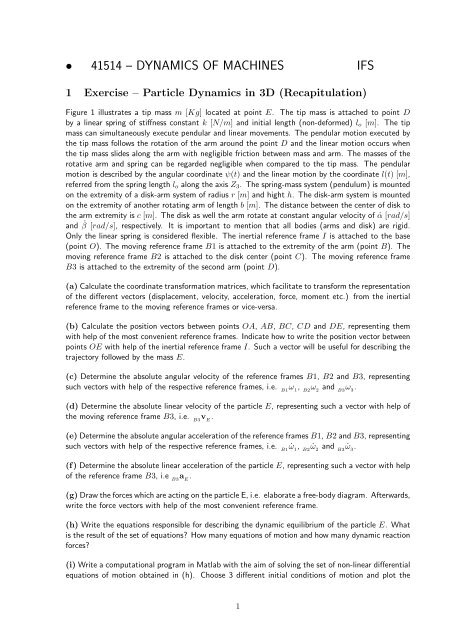
Figure 1 illustrates a tip mass m [Kg] located at point E. The tip mass is attached to point D
by a linear spring of stiffness constant k [N/m] and initial length (non-deformed) lo [m]. The tip
mass can simultaneously execute pendular and linear movements. The pendular motion executed by
the tip mass follows the rotation of the arm around the point D and the linear motion occurs when
the tip mass slides along the arm with negligible friction between mass and arm. The masses of the
rotative arm and spring can be regarded negligible when compared to the tip mass. The pendular
motion is described by the angular coordinate ψ(t) and the linear motion by the coordinate l(t) [m],
referred from the spring length lo along the axis Z3. The spring-mass system (pendulum) is mounted
on the extremity of a disk-arm system of radius r [m] and hight h. The disk-arm system is mounted
on the extremity of another rotating arm of length b [m]. The distance between the center of disk to
the arm extremity is c [m]. The disk as well the arm rotate at constant angular velocity of ˙α [rad/s]
and ˙ β [rad/s], respectively. It is important to mention that all bodies (arms and disk) are rigid.
Only the linear spring is considered flexible. The inertial reference frame I is attached to the base
(point O). The moving reference frame B1 is attached to the extremity of the arm (point B). The
moving reference frame B2 is attached to the disk center (point C). The moving reference frame
B3 is attached to the extremity of the second arm (point D).
(a)Calculatethecoordinatetransformationmatrices, whichfacilitatetotransformtherepresentation
of the different vectors (displacement, velocity, acceleration, force, moment etc.) from the inertial
reference frame to the moving reference frames or vice-versa.
(b) Calculate the position vectors between points OA, AB, BC, CD and DE, representing them
with help of the most convenient reference frames. Indicate how to write the position vector between
points OE with help of the inertial reference frame I. Such a vector will be useful for describing the
trajectory followed by the mass E.
(c) Determine the absolute angular velocity of the reference frames B1, B2 and B3, representing
such vectors with help of the respective reference frames, i.e. B1 ω 1 , B2 ω 2 and B3 ω 3 .
(d) Determine the absolute linear velocity of the particle E, representing such a vector with help of
the moving reference frame B3, i.e. B3 v E .
(e)DeterminetheabsoluteangularaccelerationofthereferenceframesB1, B2andB3, representing
such vectors with help of the respective reference frames, i.e. B1 ˙ω 1 , B2 ˙ω 2 and B3 ˙ω 3 .
(f) Determine the absolute linear acceleration of the particle E, representing such a vector with help
of the reference frame B3, i.e B3 a E .
(g)DrawtheforceswhichareactingontheparticleE,i.e. elaborateafree-bodydiagram. Afterwards,
write the force vectors with help of the most convenient reference frame.
(h) Write the equations responsible for describing the dynamic equilibrium of the particle E. What
is the result of the set of equations? How many equations of motion and how many dynamic reaction
forces?
(i) Write a computational program in Matlab with the aim of solving the set of non-linear differential
equations of motion obtained in (h). Choose 3 different initial conditions of motion and plot the
1

variables l(t) and ψ(t) as a function of time. Plot the trajectory of the particle for the different initial
conditions. Plot the dynamic reaction force as a function of time for the 3 different initial conditions.
Figure1: Spring-mass system (pendulum) attached to the rotating reference frame B3 performing
three consecutive rotations.
2

SOLUTION:
(a) Coordinate transformation matrices.
First rotation around the Z-axis of inertial reference
frame.
Second rotation around the Z1-axis of the moving
reference frame B1.
3
• Coordinate transformation matrices between
I and B1:
⎡ ⎤
cosα sinα 0
Tα = ⎣ −sinα cosα 0 ⎦
0 0 1
B1 s = Tα · I s
I s = TT α · B1 s
• Coordinate transformation matrices between
B1 and B2:
⎡ ⎤
cosβ sinβ 0
Tβ = ⎣ −sinβ cosβ 0 ⎦
0 0 1
B2 s = Tβ · B1 s
B1 s = TT β · B2 s

Third rotation around the X2-axis of the moving
reference frame B2.
(b) Position vectors.
• position vector I r OA :
IrOA = 0 0 a ⎧ ⎫
⎨ 0 ⎬
T
= 0
⎩ ⎭
a
• position vector B1 r AB :
B1 r AB = 0 b 0 T
• position vector B2 r BC :
B2 r BC = 0 0 c T
• position vector B2 r CD :
B2 r CD = 0 r h T
• position vector B3 r DE :
B3 r DE = 0 0 −(l0 +l) T
• Coordinate transformation matrices between
B2 and B3:
⎡
Tψ = ⎣
B3 s = Tψ · B2 s
1 0 0
0 cosψ sinψ
0 −sinψ cosψ
B2 s = TT ψ · B3 s
The position vectors were written with help of the most convenient reference frames, it means using
the reference frame in which their representation are the most compact one. For describing the
particle trajectory is necessary to write the vector I r OE , i.e.
I r OE = I r OA + I r AB + I r BC + I r CD + I r DE
4
⎤
⎦

or
I r OE = I r OA +TT α · B1 r AB +T T α · T T β · ( B2 r BC + B2 r CD )+TT α · T T β · TT ψ · B3 r DE
(c) Absolute angular velocity of the moving reference frames.
• Absolute angular velocity of the moving reference frame B1:
B1ω1 = Tα
⎡ ⎤⎧
⎫
cosα sinα 0 ⎨ 0 ⎬
I ˙α = ⎣ −sinα cosα 0 ⎦ 0
⎩ ⎭
0 0 1 ˙α
⇒B1 ω1 =
⎧ ⎫
⎨ 0 ⎬
0
⎩ ⎭
˙α
[rad/s]
• Absolute angular velocity of the moving reference frame B2:
B2 ω 2 = TβTα I ˙α+Tβ B1 ˙ β =
⎡
= ⎣
B2 ω 2 =
cos(α+β) sin(α+β) 0
−sin(α+β) cos(α+β) 0
0 0 1
⎧
⎨
⎩
0
0
˙α+ ˙ β
⎫
⎬
⎭ [rad/s]
⎤⎧
⎨
⎦
⎩
0
0
˙α
⎫
⎬
⎭ +
⎡
⎣
cosβ sinβ 0
−sinβ cosβ 0
0 0 1
• Absolute angular velocity of the moving reference frame B3:
B3 ω 3 = TψTβTα I ˙α+TψTβ B1 ˙ β +Tψ B2 ˙ ψ
= Tψ( B2 ω 2 + B2 ˙ ψ) =
⎡
⎣
1 0 0
0 cosψ sinψ
0 −sinψ cosψ
(d) Absolute linear velocity of the particle E.
• Absolute linear velocity of point B
B1 v B = B1 ω 1 × B1 r AB
⎤⎧
⎨
⎦
⎩
⎤⎧
⎨
⎦
⎩
0
0
˙β
⎫
⎬
⎭
˙ψ
0
˙α+ ˙ ⎫
⎬
⎭
β
=
⎧
⎨ ˙ψ
(˙α+
⎩
˙ β)sinψ
(˙α+ ˙ ⎫
⎬
⎭
β)cosψ
[rad/s]
5

=
i 1 j 1 k 1
0 0 ˙α
0 b 0
=
⎧
⎨
⎩
−b˙α
0
0
⎫
⎬
⎭ [rad/s]
•Absolute linear velocity of point C
B1 v C = B1 v B ⇒ B2 v C = Tβ B1 v B
⎡
= ⎣
cosβ sinβ 0
−sinβ cosβ 0
0 0 1
⎤⎧
⎨
⎦
⎩
−b˙α
0
0
•Absolute linear velocity of point D
B2vD = B2 vC + B2 ω2 × B2 rCD + B2vrel
=0
⎧
⎨
=
⎩
−b˙αcosβ
b˙αsinβ
0
⎫
⎬
⎭ +
i 2 j 2 k 2
0 0 ˙α+ ˙ β
0 r h
•Absolute linear velocity of the particle E
B3vE = B3vD + B3ω3 × B3 rDE • (I)
I
B3 v D = Tψ B2 v D
B3 v D =
• (II)
⎡
⎣
B3 ω 3 × B3 r DE
II
1 0 0
0 cosψ sinψ
0 −sinψ cosψ
⎫
⎬
⎭ ⇒B2 vC =
⎧
⎨
⎩
+ B3 v rel
III
⎤⎧
⎨
⎦
⎩
=
⎧
⎨
⎩
−b˙αcosβ
b˙αsinβ
0
⎫
⎬
−b˙αcosβ −r(˙α+ ˙ β)
b˙αsinβ
0
−b˙αcosβ −r(˙α+ ˙ β)
b˙αsinβ
0
6
⎫
⎬
⎭ =
⎧
⎨
⎩
⎭ [m/s]
⎫
⎬
⎭ [m/s]
−b˙αcosβ −r(˙α+ ˙ β)
b˙αsinβcosψ
−b˙αsinβsinψ
⎫
⎬
⎭ [m/s]

=
i 3 j 3 k 3
˙ψ (˙α+ ˙ β)sinψ (˙α+ ˙ β)cosψ
0 0 −(l0 +l)
• (III)
B1 v rel =
⎧
⎨
⎩
0
0
− ˙ l
⎫
⎬
⎭
• (I)+(II)+(III)
B3 v E =
⎧
⎨
⎩
=
⎧
⎨
⎩
−(l0 +l)(˙α+ ˙ β)sinψ
(l0 +l) ˙ ψ
0
−b˙αcosβ −r(˙α+ ˙ β)−(l0 +l)(˙α+ ˙ β)sinψ
b˙αsinβcosψ +(l0 +l) ˙ ψ
−b˙αsinβsinψ − ˙ l
⎫
⎬
⎭ [m/s]
(e) Absolute angular acceleration of the moving reference frames.
• Absolute angular acceleration of the moving reference frame B1:
B1 ˙ω d
1 =
dt ( B1ω1 )+ B1ω1 × B1 ω ⎧ ⎫
⎨ 0 ⎬
1 = 0
⎩ ⎭
=0 ¨α
⇒B1 ˙ω 1 =
⎧ ⎫
⎨ 0 ⎬
0
⎩ ⎭
0
[rad/s2 ]
• Absolute angular acceleration of the moving reference frame B2:
B2 ˙ω d
2 =
dt ( B2ω2 )+ B2ω2 × B2 ω ⎧
⎨ 0
2 = 0
⎩
=0 ¨α+ ¨ ⎫
⎬
⎭
β
⇒B2 ˙ω 2 =
⎧ ⎫
⎨ 0 ⎬
0
⎩ ⎭
0
[rad/s2 ]
• Absolute angular acceleration of the moving reference frame B3:
B3 ˙ω 3
B3 ˙ω 3 =
d
=
dt ( B3ω3 )+ B3ω3 × B3 ω3 =
=0
⎧
⎨
⎩
¨ψ
(¨α+ ¨ β)sinψ +(˙α+ ˙ β) ˙ ψcosψ
(¨α+ ¨ β)cosψ −(˙α+ ˙ β) ˙ ψsinψ
⎫
⎬
⎫
⎬
⎭ ⇒B3 ˙ω 3 =
⎧
⎨ ¨ψ
(˙α+
⎩
˙ β) ˙ ψcosψ
−(˙α+ ˙ β) ˙ ⎫
⎬
⎭
ψsinψ
[rad/s2 ]
It is important to point out that ¨α = ¨ β = 0! It is given in the beginning of the example, when the
7
⎭

problem was formulated.
(f) Absolute linear acceleration of the point B.
B1aB = B1aO + B1ω1 ×( B1ω1 × B1rOB )+ B1 ˙ω 1 × B1rOB +2 · B1ω1 × B1vrel
=0
=0
B1 ω 1 ×
B1 a B =
⎧
⎨
⎩
i 1 j 1 k 1
0 0 ˙α
0 b a
0
−b˙α 2
0
⎫
⎬
=
⎭ [m/s2 ]
i 1 j 1 k 1
0 0 ˙α
−b˙α 0 0
(g) Absolute linear acceleration of the point C.
B1 a C = B1 a B ⇒ B2 a C = Tβ B1 a B
⎡
= ⎣
cosβ sinβ 0
−sinβ cosβ 0
0 0 1
⎤⎧
⎨
⎦
⎩
0
−b˙α 2
0
=
⎧
⎨ 0
−b˙α
⎩
2
⎫
⎬
⎭
0
⎫
⎬
⎭ ⇒B2 aC =
⎧
⎨
⎩
(g) Absolute linear acceleration of the particle E.
−b˙α 2 sinβ
−b˙α 2 cosβ
0
⎫
⎬
⎭ [m/s2 ]
=0
B3aE = B3aD + B3ω3 × ( B3ω3 × B3rDE ) + B3 ˙ω 3 × B3rDE + 2 · B3ω3 × B3vrel
(I) (II)
(III)
• (I)
B2aD = B2aC
see item (f)
(IV)
+ B1 a rel
=0
+ B3 a rel
(V)
+ B2ω2 × ( B2ω2 × B2rCD ) + B2 ˙ω 2 × B2rCD +2 · B2ω2 × B2vrel
(VI)
8
=0
=0
+ B2 a rel
=0

• (VI)
B2 ω 2 ×
⇒ B2 a D =
i 2 j 2 k 2
0 0 (˙α+ ˙ β)
0 r h
⎧
⎨
⎩
B3 a D = Tψ B2 a D =
B3 a D =
• (II)
B3 ω 3 ×
⇒
⎧
⎨
⎩
=
−b˙α 2 sinβ
−b˙α 2 cosβ −r(˙α+ ˙ β) 2
0
⎡
⎣
i 2 j 2 k 2
0 0 (˙α+ ˙ β)
−r(˙α+ ˙ β) 0 0
1 0 0
0 cosψ sinψ
0 −sinψ cosψ
⎫
⎬
−b˙α 2 sinβ
−(b˙α 2 cosβ +r(˙α+ ˙ β) 2 )cosψ
(b˙α 2 cosβ +r(˙α+ ˙ β) 2 )sinψ
i 3 j 3 k 3
˙ψ (˙α+ ˙ β)sinψ (˙α+ ˙ β)cosψ
0 0 −(l0 +l)
⎭ [rad/s2 ]
⎤⎧
⎨
⎦
⎩
⎫
⎬
=
⎧
⎨ 0
−r(˙α+
⎩
˙ β) 2
⎫
⎬
⎭
0
−b˙α 2 sinβ
−b˙α 2 cosβ −r(˙α+ ˙ β) 2
0
⎭ [rad/s2 ]
=
i 3 j 3 k 3
˙ψ (˙α+ ˙ β)sinψ (˙α+ ˙ β)cosψ
−(l0 +l)(˙α+ ˙ β)sinψ (l0 +l) ˙ ψ 0
• (III)
B3 ˙ω 3 × B3 r DE =
2 ·
• (IV)
i 3 j 3 k 3
¨ψ (˙α+ ˙ β) ˙ ψcosψ −(˙α+ ˙ β) ˙ ψsinψ
0 0 −(l0 +l)
i 3 j 3 k 3
˙ψ (˙α+ ˙ β)sinψ (˙α+ ˙ β)cosψ
0 0 − ˙ l
=
⎧
⎨
⎩
=
⎧
⎨
⎩
=
⎧
⎨
⎩
−2 ˙ l(˙α+ ˙ β) ˙ ψsinψ
2 ˙ l ˙ ψ
0
9
⎫
⎬
⎭
−(l0 +l) ˙ ψ(˙α+ ˙ β)cosψ
−(l0 +l)(˙α+ ˙ β) 2 sinψcosψ
(l0 +l)( ˙ ψ 2 +(˙α+ ˙ β) 2 sin 2 ψ)
−(l0 +l)(˙α+ ˙ β) ˙ ψcosψ
(l0 +l) ¨ ψ
0
⎫
⎬
⎭
⎫
⎬
⎭
⎫
⎬
⎭

B3
B3P =
• (V)
B3 a rel =
⎧
⎨
⎩
0
0
− ¨ l
⎫
⎬
⎭ [m/s2 ]
Adding the terms determined in (I), (II), (III), (IV) and (V), one achieves the absolute linear acceleration
of the particle E represented in the reference frame B3:
B3 a E =
⎧
⎨
⎩
−b˙α 2 sinβ −2(l0 +l) ˙ ψ(˙α+ ˙ β)cosψ −2 ˙ l(˙α+ ˙ β)sinψ
−(b˙α 2 cosβ +r(˙α+ ˙ β) 2 )cosψ −(l0 +l)(˙α+ ˙ β) 2 sinψcosψ +(l0 +l) ¨ ψ +2 ˙ l ˙ ψ
(b˙α 2 cosβ +r(˙α+ ˙ β) 2 )sinψ +(l0 +l)( ˙ ψ 2 +(˙α+ ˙ β) 2 sin 2 ψ)− ¨ l
(g) Free-body diagram of the particle E.
⎫
⎬
⎭ [rad/s2 ]
• Vector representation of the forces acting on the particle E :
I P = 0 0 −mg T
• Force in the direction of the pendulum rod
B3 T = 0 0 kl T
• Forces perpendicular to the pendulum rod:
B3 R = −R 0 0 T
(h) Dynamic equilibrium of the particle E according to the second Newton’s law:
d
F = TψTβTα
dt (m I v E ) = TψTβTα( ˙m
=0
B3 F = m B3 a E = B3 R + B3 T+TψTβTα I P
⎡
⎣
1 0 0
0 cosψ sinψ
0 −sinψ cosψ
⎤⎡
⎦⎣
cosβ sinβ 0
−sinβ cosβ 0
0 0 1
I v E +m I a E )
⎤⎡
⎦⎣
10
cosα sinα 0
−sinα cosα 0
0 0 1
⎤⎧
⎨
⎦
⎩
0
⎫
⎬
0
⎭
−mg
=
⎧
⎨ 0
⎫
⎬
−mgsinψ
⎩ ⎭
−mgcosψ

⎧
⎨
⎩
⎧
⎨
m
⎩
−R
−mgsinψ
−mgcosψ +kl
⎫
⎬
⎭ =
−b˙α 2 sinβ −2(l0 +l) ˙ ψ(˙α+ ˙ β)cosψ −2 ˙ l(˙α+ ˙ β)sinψ
−(b˙α 2 cosβ +r(˙α+ ˙ β) 2 )cosψ −(l0 +l)(˙α+ ˙ β) 2 sinψcosψ +(l0 +l) ¨ ψ +2 ˙ l ˙ ψ
(b˙α 2 cosβ +r(˙α+ ˙ β) 2 )sinψ +(l0 +l)( ˙ ψ 2 +(˙α+ ˙ β) 2 sin 2 ψ)− ¨ l
The final result of the application of the second Newton’s law is the achievement of three equations,
i.e. one for calculating the dynamic reaction forces R and two additional equations responsible for
describing the movement of the particle E as a function of the time, ¨ ψ(t) and ¨ l(t).
• Dynamic reaction force (direction X 3 ) :
R = m(b˙α 2 sinβ +2(l0 +l) ˙ ψ(˙α+ ˙ β)cosψ +2 ˙ l(˙α+ ˙ β)sinψ)
• Equations of motion for the particle E (directions Y 3 and Z 3 )
¨ψ = − g
(l0 +l) sinψ + (b˙α2 cosβ +r(˙α+ ˙ β) 2 )
(l0 +l)
cosψ +(˙α+ ˙ β) 2 sinψcosψ − 2˙ l ˙ ψ
(l0 +l)
¨ l = − k
m l+gcosψ +[b˙α2 cosβ +r(˙α+ ˙ β) 2 ]sinψ +(l0 +l)[ ˙ ψ 2 +(˙α+ ˙ β) 2 sin 2 ψ]
(i) Computational routine implemented using Matlab and numerical results.
clear all close all
% parameters of the mechanical system
a = 0.05; % [m]
b = 0.5; % [m]
c = 0.05; % [m]
r = 0.1; % [m]
h = 0.20; % [m]
lo= 0.1; % [m]
m = 0.2; % [kg]
k = 2000; % [N/m]
g = 9.82; % [m/s^2]
% initial conditions
alfa(1) = 0 % [rad]
beta(1) = 0 % [rad]
alfad = 2*pi/2 % [rad/s]
betad = 2*pi*4 % [rad/s]
l(1) = 0.000; % [m]
ld(1) = 0; % [m/s]
psi(1) = pi/6; % [rad]
psid(1) = 0; % [rad/s]
11
⎫
⎬
⎭

% defining the position vectors with respect to desired reference frames
Iroa = [0; 0; a];
B1rab = [0; b; 0];
B2rbc = [0; 0; c];
B2rcd = [0; r; h];
B3rde = [0; 0; -(lo+l(1))];
% defining the transformation matrices
Talfa = [cos(alfa(1)) sin(alfa(1)) 0
-sin(alfa(1)) cos(alfa(1)) 0
0 0 1];
Tbeta = [cos(beta(1)) sin(beta(1)) 0
-sin(beta(1)) cos(beta(1)) 0
0 0 1];
Tpsi = [1 0 0
0 cos(psi(1)) sin(psi(1));
0 -sin(psi(1)) cos(psi(1))];
% creating the position vector which describes mass m’s trajectory in the inertial frame
roe = Iroa + Talfa’*B1rab + Talfa’*Tbeta’*(B2rbc+B2rcd) + Talfa’*Tbeta’*Tpsi’*B3rde;
rx(1)= roe(1);
ry(1)= roe(2);
rz(1)= roe(3);
% calculating the reaction force R represented in the X3 direction
Reaction(1) = m*( b*alfad^2*sin(beta(1)) ...
+ 2*(lo+l(1))*psid(1)*(alfad+betad)*cos(psi(1)) ...
+ 2*ld(1)*(alfad+betad)*sin(psi(1)));
% numerical solution
% time step
deltaT = 0.00005;
% number of integration points
n_int = 60000;
for i=2:n_int,
%tempo=(i-2)*deltaT
t_int(i-1) = (i-2)*deltaT;
% accelerations
psidd(i-1) = -g/(lo+l(i-1))*sin(psi(i-1)) + ...
(b*alfad^2*cos(beta(i-1))+r*(alfad+betad)^2)/(lo+l(i-1))*cos(psi(i-1)) + ...
(alfad+betad)^2*sin(psi(i-1))*cos(psi(i-1)) - ...
2*ld(i-1)*psid(i-1)/(lo+l(i-1));
ldd(i-1) = -k/m*l(i-1) ...
+ (g*cos(psi(i-1))+(b*alfad^2*cos(beta(i-1))) ...
+ r*(alfad+betad)^2)*sin(psi(i-1)) ...
+ (lo+l(i-1))*(psid(i-1)^2+(alfad+betad)^2*sin(psi(i-1))^2);
% velocities
12

end
alfa(i) = alfa(i-1) + alfad*deltaT;
beta(i) = beta(i-1) + betad*deltaT;
psid(i) = psid(i-1) + psidd(i-1)*deltaT;
ld(i) = ld(i-1) + ldd(i-1)*deltaT;
% displacements
psi(i) = psi(i-1) + psid(i-1)*deltaT;
l(i) = l(i-1) + ld(i-1)*deltaT;
% reaction force
Reaction(i) = m*( b*alfad^2*sin(beta(i)) ...
+ 2*(lo+l(i))*psid(i)*(alfad+betad)*cos(psi(i)) ...
- 2*ld(i)*(alfad+betad)*sin(psi(i)));
% transformation matrices
Talfa = [ cos(alfa(i)) sin(alfa(i)) 0
-sin(alfa(i)) cos(alfa(i)) 0
0 0 1];
Tbeta = [ cos(beta(i)) sin(beta(i)) 0
-sin(beta(i)) cos(beta(i)) 0
0 0 1];
Tpsi = [1 0 0
0 cos(psi(i)) sin(psi(i))
0 -sin(psi(i)) cos(psi(i))];
% defining the position vectors with respect to desired reference frames
Iroa = [0; 0; a];
B1rab = [0; b; 0];
B2rbc = [0; 0; c];
B2rcd = [0; r; h];
B3rde = [0; 0; -(lo+l(i))]; % observe that only B3rde is time dependent!
% creating the position vector which describes mass m’s trajectory in the inertial frame
roe = Iroa + Talfa’*B1rab + Talfa’*Tbeta’*(B2rbc+B2rcd) + Talfa’*Tbeta’*Tpsi’*B3rde;
rx(i)= roe(1);
ry(i)= roe(2);
rz(i)= roe(3);
nplot=n_int-1;
figure(1)
plot(t_int(1:nplot),l(1:nplot))
grid
xlabel(’time [s]’)
ylabel(’l(t) [s]’)
figure(2)
plot(t_int(1:nplot),psi(1:nplot))
grid
xlabel(’time [s]’)
ylabel(’\psi(t) [s]’)
figure(3)
plot3(rx,ry,rz)
axis([-0.8 0.8 -0.8 0.8 0 0.4])
13

xlabel(’x [m]’)
ylabel(’y [m]’)
zlabel(’z [m]’)
grid
figure(4)
plot(t_int(1:nplot),Reaction(1:nplot))
grid
xlabel(’time [s]’)
ylabel(’R(t) [N]’)
Figure 1 illustrates the results obtained aided by the computational routine implemented using Matlab.
(a)
l(t) [s]
0.04
0.035
0.03
0.025
0.02
0.015
0.01
0.005
0
−0.005
−0.01
0 0.5 1 1.5
time [s]
2 2.5 3
(c) (d)
(b)
ψ(t) [s]
3
2.5
2
1.5
1
0.5
0
0 0.5 1 1.5
time [s]
2 2.5 3
Figure 2: (a) Angle ψ(t) as function of time; (b) displacement l(t) as function of time; (c)
trajectory described by the particle E when the arm and the disk rotate with a constant angular
velocity given in the Matlab routine; (d) reaction force R(t) as function of time.
14