Lexical variation in aggregate perspective

More documents

Recommendations

Info

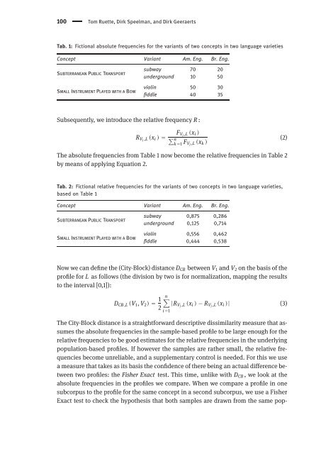
100 Tom Ruette, Dirk Speelman, and Dirk Geeraerts Tab. 1: Fictional absolute frequencies for the variants of two concepts in two language varieties Concept Variant Am. Eng. Br. Eng. SUBTERRANEAN PUBLIC TRANSPORT SMALL INSTRUMENT PLAYED WITH A BOW subway 70 20 underground 10 50 violin 50 30 fiddle 40 35 Subsequently, we introduce the relative frequency R : RVj ,L (xi ) = FVj ,L (xi ) n k =1 FVj ,L (xk ) The absolute frequencies from Table 1 now become the relative frequencies in Table 2 by means of applying Equation 2. Tab. 2: Fictional relative frequencies for the variants of two concepts in two language varieties, based on Table 1 Concept Variant Am. Eng. Br. Eng. SUBTERRANEAN PUBLIC TRANSPORT SMALL INSTRUMENT PLAYED WITH A BOW subway 0,875 0,286 underground 0,125 0,714 violin 0,556 0,462 fiddle 0,444 0,538 Now we can define the (City-Block) distance DCB between V1 and V2 on the basis of the profile for L as follows (the division by two is for normalization, mapping the results to the interval [0,1]): DCB ,L (V1, V2) = 1 2 n i =1 (2) |RVj ,L (xi ) − RVj ,L (xi )| (3) The City-Block distance is a straightforward descriptive dissimilarity measure that assumes the absolute frequencies in the sample-based profile to be large enough for the relative frequencies to be good estimates for the relative frequencies in the underlying population-based profiles. If however the samples are rather small, the relative frequencies become unreliable, and a supplementary control is needed. For this we use a measure that takes as its basis the confidence of there being an actual difference between two profiles: the Fisher Exact test. This time, unlike with DCB , we look at the absolute frequencies in the profiles we compare. When we compare a profile in one subcorpus to the profile for the same concept in a second subcorpus, we use a Fisher Exact test to check the hypothesis that both samples are drawn from the same pop-
Lexical variation in aggregate perspective 101 ulation. We use the p-value from the Fisher Exact test as a filter for DCB .Wesetthe dissimilarity between subcorpora at zero if p > 0.05, and we use DCB if p < 0.05. 2 If we now apply this step to the fictional data from Table 1 and 2, we must first calculate the Fisher Exact p value for every concept, verifying that the absolute frequencies for American and British English are sampled from different populations. For SUBTERRANEAN PUBLIC TRANSPORT,thepvalueismuchsmallerthan0.05,sowecanac cept that British English is different from American English when it comes to this concept. Therefore, we calculate the City-Block distance by means of Equation 5 for SUB- TERRANEAN PUBLIC TRANSPORT. Filling in the equation, we get 0.5 × [(|0.875–0.286|) + (|0.125–0.714|)] = 0.589. For the concept of a SMALL INSTRUMENT PLAYED WITH A BOW we find a p value for the Fisher Exact test larger than 0.05, so we can say that British English is statistically speaking not a different population than American English. Therefore, we can set the distance between these varieties for this concept at zero. To calculate the dissimilarity between subcorpora on the basis of many profiles, we just sum the dissimilarities for the individual profiles. In other words, given a set of profiles L1 to Lm , then the global dissimilarity D between two subcorpora V1 and VL2 on the basis of L1 up to Lm can be calculated as: DCB (V1, V2) = m (L −i (V1, V2)W (Li )) (4) i =1 The W in the formula is a weighting factor. We use weights to ensure that concepts which have a relatively higher frequency (summed over the size of the two subcorpora that are being compared) 3 also have a greater impact on the distance measurement. In other words, in the case of a weighted calculation, concepts that are more common in everyday life and language are treated as more important. Applying this to the fictional example from Table 1, we can calculate the W per concept by dividing the sum of the absolute frequencies of all variants for one concept by the sum of simply all variations. For SUBTERRANEAN PUBLIC TRANSPORT this equals to (70+10+20+50)/(70+10+20+50+ 50 + 40 + 30 + 35) = 0.492. There is no need to calculate the W for SMALL INSTRUMENT PLAYED WITH A BOW as its distance is already set to zero. Filling out equation 4, we find that the distance between British English and American English aggregated over both concepts is (0.589 × 0.492) + 0 = 0.29. Now, we put text categorization in contrast with the profile-based approach, which incorporates probabilistic information of word choice. In text categorization, noncategorical (probabilistic) word choice is well accounted for (unlike dialectometric ap- 2 If the frequency of the profile was lower than 30 in the two varieties that are being compared, that profile was excluded from the comparison. 3 The size of the two subcorpora is not the actual amount of words in the two subcorpora, but the sum of all profiles in these two subcorpora with a frequency higher than 30.
Page 1 and 2: Tom Ruette, Dirk Speelman, and Dirk
Page 3 and 4: Lexical variation in aggregate pers
Page 5: Lexical variation in aggregate pers
Page 19 and 20: Appendix Lexical variation in aggre
Page 21 and 22: qnp.be.e.0 qnp.be.e.1 qnp.be.p.0 qn

Lexical variation in aggregate perspective

You also want an ePaper? Increase the reach of your titles

Delete template?

Save as template?