Hilding Elmqvist, Hubertus Tummescheit and Martin Otter ... - Modelica

More documents

Recommendations

Info

H. Elmqvist, H. Tummescheit, M. Otter Object-Oriented Modeling of Thermo-Fluid Systems 6.1 High Accuracy Water Model IF97 The Modelica_Media library contains a very detailed medium model of water in the liquid, gas and two phase region based on the IF97 standard [6]. It is an adapted and slightly improved version from the ThermoFluid library (Tummescheit and Eborn (2001), Tummescheit (2002)). High accuracy thermodynamic properties of fluids are modeled with two kinds of multiparameter, fundamental equations of state: • An equation for the specific Helmholtz free energy f(ρ,T) or f(v=1/ρ,T) • An equation for the Gibbs free enthalpy g(p,T) For numerical reasons the fundamental equations use dimensionless variables which are most often scaled with the critical parameters. The IF97 industrial steam tables uses both equation types and furthermore divides the overall fluid state into 5 regions in order to achieve high accuracy everywhere with a lower number of parameters. In spite of the complexities of the underlying formulation, the user interface for calling the properties is very simple. The medium interface is implemented with utility functions that have a simple interface, e.g. rho = Water.IF97.rho_ph(p,h); //density T = WaterIF97.T(p,h); //temperature s = WaterIF97.s_ph(p,h); //specific entropy Common sub-expression elimination and nested inlining of function calls ensure that the computationally expensive call to one of the fundamental equations happens only once. A record containing the fundamental derivatives of the equation of states is used by Dymola in the common sub-expression elimination and is thus only computed once. The fundamental derivatives for the free Helmholtz energy f(ρ,T) are: p = ρ f s p = − T f 2 = ρ ρ T 2 fTρ 2 ∂f = ρ ∂ρ 2 T pρ = 2ρf ρ + ρ f ρρ cv = −TfTT Here the short subscript notation is used for partial derivatives, see explanation above. A similar set of fundamental derivatives exists for the Gibbs free enthalpy g(p,T): s = −g v = g v v c T p p p = g = g T pT pp = −Tg pp From these fundamental derivatives, all other partial derivatives of thermodynamic properties with respect to other properties can be computed using thermodynamic determinants, e.g. 2 ρ ρ( cvρ + pT ) ∂ρ ρ pT = , = 2 2 2 p ρ pρcv + TpT ∂h ρ pρcv + ∂ 2 ∂ h p TpT When needed, e.g. for index reduction to change the states to numerically favorable ones, these partial derivatives can be computed with minimal effort from the fundamental derivatives in the property record. In order to add other Helmholtz-or Gibbsbased equations of state to Modelica_Media, only the fundamental derivatives need to be computed, the functions to compute the standard properties are part of the library. The partial derivatives are used in two situations where the Modelica_Media properties provide unique features for efficiency and model order reduction. For all property calls that may have to be differentiated for index reduction, efficient derivative functions are provided. A very useful model order reduction for large two-phase heat exchangers is to equate the metal mass and boiling water temperatures, e.g. as in the drum Boiler model in [3]. Equating the temperatures leads to an index reduction problem. The algorithm for index reduction needs to compute the time derivative of temperature as a function of the time derivatives of the states. When pressure p and specific enthalpy h are the states, the expansion reads: dT dt ∂T = ∂p h ∂T + ∂h p if in single phase dT ∂Tsat = if in the two phase region dt ∂p These derivatives are automatically computed when needed without user interaction. This allows writing the equations in the most natural form, as demonstrated in [3]. The same algorithmic procedure is used to transform the “natural” form of the mass- and energy balances into equations using the input to the property routines as states. The Modelica Association Modelica 2003, November 3-4, 2003
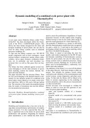
H. Elmqvist, H. Tummescheit, M. Otter Object-Oriented Modeling of Thermo-Fluid Systems Density [kg/m3] 1000 100 10 0.1 200 1 400 1000 Density as a Function of Enthalpy and Pressure x = 0 2000 Enthalpy [kJ/kg] 4000 1 x = 1 10 Pressure [bar] 100 Figure 7: log.-plot of ρ(p,h) for IF97 water 1000 6.2 High Accuracy Ideal Gas Models Ideal gas properties cover a broad range of interesting engineering applications: air conditioning and climate control, industrial and aerospace gas turbines, combustion processes, automotive engines, fuel cells and many chemical processes. Critically evaluated parameter sets are available for a large number of substances. The coefficients and data used in the Modelica_Media library are from [9]. Care has been taken to enable users to create their own gas mixtures with minimal effort. For most gases, the region of validity is from 200 K to 6000 K, sufficient for most technical applications. The equation of state consists of the well-known ideal gas law p = ρ ⋅ R ⋅T with R the specific gas constant, and polynomials for the specific heat capacity cp (T ) , the specific enthalpy h(T ) and the specific entropy s ( T, p) : cp( T ) = R ∑ i= 1 ⎛ a h( T ) = RT⎜ ⎜ − ⎝ T 7 a T i 1 2 i−3 + a 2 log( T ) + T 7 ∑ i= 3 ⎛ a ⎜ 1 a2 s0 ( T ) = R ⎜ − − + a3 log( T ) + 2 ⎝ 2T T ⎛ p ⎞ s( T, p) = s − ⎜ ⎟ 0( T ) Rln ⎝ p0 ⎠ i−3 T b ⎞ 1 a + ⎟ i i − 2 T ⎟ ⎠ 7 ∑ i= 4 i−3 T ⎞ a + ⎟ i b2 i − 3 ⎟ ⎠ The polynomials for h (T ) and s0 ( T ) are derived via integration from the one for cp(T ) and contain the integration constants b 1,b2 that define the reference specific enthalpy and entropy. For entropy differences the reference pressure p0 is arbitrary, but not for absolute entropies. It is chosen as 1 standard atmosphere (101325 Pa). Depending on the intended use of the properties, users can choose between different reference enthalpies: 1. The enthalpy of formation Hf of the molecule can be included or excluded. 2. The value 0 for the specific enthalpy without Hf can be defined to be at 298.15 K (25 °C) or at 0 K. For some of the species, transport properties are also available. The form of the equations is: ⎛ ν ⎞ B C lg⎜ ⎟ = A⋅ lg( T ) + + + D k 2 ⎝10 ⎠ T T Bλ Cλ lg( λ) = Aλ ⋅ lg( T ) + + + D 2 λ T T η = ν ⋅ ρ with the kinematic viscosity ν , dynamic viscosity η , thermal conductivity λ and parameters A,B,C,D and k. Note, though, that the thermal conductivity is only the “frozen” thermal conductivity, i.e., not valid for fast reactions. 6.3 Ideal Gas Mixtures For mixtures of ideal gases, the standard, ideal mixing rules apply: h s mix mix ( T ) = ( T ) = nspecies ∑ i= 1 nspecies ∑ i= 1 h ( T ) x i ⎛ p ⎞ ⎜ ⎟ ⎝ p0 ⎠ ( s ( T ) − R ln( y ) ) x − Rln⎜ ⎟, i i where the xi are the mass fractions, the Ri are the specific gas constants and the yi are the molar fractions of the components of the mixture. Most other properties are then computed just as for single species media. Dynamic viscosity and thermal conductivity for mixtures require interaction parameters of a similar functional form as the viscosity itself and are (not yet) implemented. For mixtures of ideal gases, three usage scenarios can be distinguished: 1. The composition is fixed and is the same throughout the system. This means that a new data record can be computed by preprocessing the component property data that can be treated as a new, single species data record (assuming ideal mixing). 2. The composition is variable, but changes in composition occur only through convection, i.e. slowly. 3. The composition is variable and may change through reactions too, i.e. composition changes are possibly very fast. Case 1 and 2 above can be handled within a single model with a Boolean switch, case 3 needs to extend from that model because usually a number of The Modelica Association Modelica 2003, November 3-4, 2003 i i i
Page 1 and 2: Proceedings of the 3 rd Internation
Page 3 and 4: H. Elmqvist, H. Tummescheit, M. Ott
Page 15: H. Elmqvist, H. Tummescheit, M. Ott
Page 19: H. Elmqvist, H. Tummescheit, M. Ott

Hilding Elmqvist, Hubertus Tummescheit and Martin Otter ... - Modelica

You also want an ePaper? Increase the reach of your titles

Delete template?

Save as template?