Hilding Elmqvist, Hubertus Tummescheit and Martin Otter ... - Modelica
Hilding Elmqvist, Hubertus Tummescheit and Martin Otter ... - Modelica
Hilding Elmqvist, Hubertus Tummescheit and Martin Otter ... - Modelica

You also want an ePaper? Increase the reach of your titles
YUMPU automatically turns print PDFs into web optimized ePapers that Google loves.
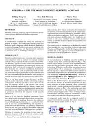
H. <strong>Elmqvist</strong>, H. <strong>Tummescheit</strong>, M. <strong>Otter</strong> Object-Oriented Modeling of Thermo-Fluid Systems<br />
correspondingly. In a future version, this selection<br />
might be performed automatically by a tool.<br />
The user can currently choose between three<br />
variants of the pressure loss model:<br />
1. Constant Laminar: pLoss = k ⋅ m&<br />
It is assumed that the flow is only laminar. The<br />
constant k is defined by providing p Loss <strong>and</strong> m&<br />
for nominal flow conditions that, for example,<br />
are determined by measurements.<br />
2. Constant Turbulent: pLoss = k ⋅ m&<br />
⋅ m&<br />
.<br />
It is assumed that the flow is only turbulent.<br />
Again, the constant k is defined by providing<br />
p Loss <strong>and</strong> m& for nominal flow conditions. For<br />
small mass flow rates, the quadratic, or in the<br />
inverse case the square root, characteristic is<br />
replaced by a cubic polynomial. This avoids the<br />
usual problems at small mass flow rates.<br />
3. Detailed Friction: provides a detailed model of<br />
frictional losses for commercial pipes with nonuniform<br />
roughness (including the smooth pipe<br />
as a special case) according to.:<br />
L<br />
pLoss = λ(Re,<br />
∆)<br />
⋅ ⋅ ρ ⋅ v⋅|<br />
v |<br />
2D<br />
2<br />
Lη<br />
= λ2<br />
(Re, ∆)<br />
⋅ = λ (Re, ∆)<br />
⋅ k<br />
3 3 2<br />
2<br />
2D<br />
ρ<br />
v ⋅ D ⋅ ρ D<br />
Re = = ⋅ m&<br />
η A⋅η<br />
with<br />
λ : friction coefficient (= 4·fm)<br />
λ2 : used friction coefficient (= λ·Re·|Re|)<br />
Re : Reynolds number.<br />
L : length of pipe<br />
A : cross-sectional area of pipe<br />
D : hydraulic diameter of pipe<br />
= 4*A/wetted perimeter<br />
(circular cross Section: D = diameter)<br />
δ : Absolute roughness of inner pipe wall<br />
(= averaged height of asperities)<br />
∆ : Relative roughness (=δ/D)<br />
ρ : density<br />
η : dynamic viscosity<br />
v : Mean velocity<br />
k2 abbreviation for Lη 2 /(2D 3 ρ 3 )<br />
Note that the Reynolds number might be negative if<br />
the velocity or the mass flow rate is negative. The<br />
"Detailed Friction" variant will be discussed in more<br />
detail, since several implementation choices are<br />
non-st<strong>and</strong>ard: The first equation above to compute<br />
the pressure loss as a function of the friction<br />
coefficient λ <strong>and</strong> the mean velocity v is usually used<br />
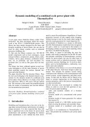
<strong>and</strong> presented in textbooks, see Figure 4. This form<br />
is not suited for a simulation program since λ =<br />
64/|Re| if |Re| < 2000, i.e., a division by zero occurs<br />
for zero mass flow rate because Re = 0 in this case.<br />
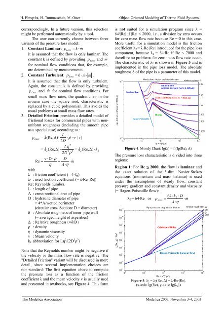
More useful for a simulation model is the friction<br />
coefficient λ2 = λ·Re·|Re| introduced for the pipe loss<br />
component, because λ2 = 64·Re if Re < 2000 <strong>and</strong><br />
therefore no problems for zero mass flow rate occur.<br />
The characteristic of λ2 is shown in Figure 5 <strong>and</strong> is<br />
implemented in the pipe loss model. The absolute<br />
roughness δ of the pipe is a parameter of this model.<br />
Figure 4. Moody Chart: lg(λ) = f (lg(Re), ∆)<br />
The pressure loss characteristic is divided into three<br />
regions:<br />
Region 1: For Re ≤ 2000, the flow is laminar <strong>and</strong><br />
the exact solution of the 3-dim. Navier-Stokes<br />
equations (momentum <strong>and</strong> mass balance) is used<br />
under the assumptions of steady flow, constant<br />
pressure gradient <strong>and</strong> constant density <strong>and</strong> viscosity<br />
(= Hagen-Poiseuille flow):<br />
64 ⋅ k2<br />
⋅ D<br />
λ2 = 64·Re or pLoss = ⋅ m&<br />
A⋅η<br />
Figure 5. λ2 = λ2(Re, ∆) = λ·Re·|Re|.<br />
(x-axis: lg(Re), y-axis: lg(λ2))<br />
The <strong>Modelica</strong> Association <strong>Modelica</strong> 2003, November 3-4, 2003