Chapter 16--Properties of Stars
Chapter 16--Properties of Stars
Chapter 16--Properties of Stars

Create successful ePaper yourself
Turn your PDF publications into a flip-book with our unique Google optimized e-Paper software.
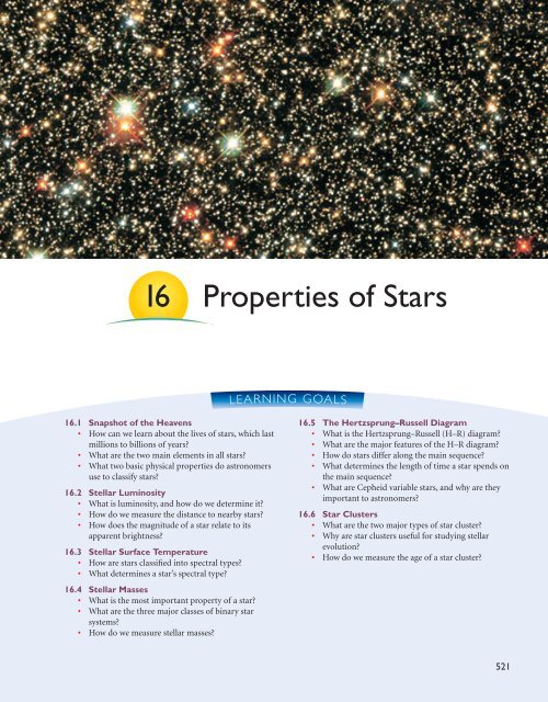
<strong>16</strong> <strong>Properties</strong> <strong>of</strong> <strong>Stars</strong><br />
<strong>16</strong>.1 Snapshot <strong>of</strong> the Heavens<br />
• How can we learn about the lives <strong>of</strong> stars, which last<br />
millions to billions <strong>of</strong> years?<br />
• What are the two main elements in all stars?<br />
• What two basic physical properties do astronomers<br />
use to classify stars?<br />
<strong>16</strong>.2 Stellar Luminosity<br />
• What is luminosity, and how do we determine it?<br />
• How do we measure the distance to nearby stars?<br />
• How does the magnitude <strong>of</strong> a star relate to its<br />
apparent brightness?<br />
<strong>16</strong>.3 Stellar Surface Temperature<br />
• How are stars classified into spectral types?<br />
• What determines a star’s spectral type?<br />
<strong>16</strong>.4 Stellar Masses<br />
• What is the most important property <strong>of</strong> a star?<br />
• What are the three major classes <strong>of</strong> binary star<br />
systems?<br />
• How do we measure stellar masses?<br />
LEARNING GOALS<br />
<strong>16</strong>.5 The Hertzsprung–Russell Diagram<br />
• What is the Hertzsprung–Russell (H–R) diagram?<br />
• What are the major features <strong>of</strong> the H–R diagram?<br />
• How do stars differ along the main sequence?<br />
• What determines the length <strong>of</strong> time a star spends on<br />
the main sequence?<br />
• What are Cepheid variable stars, and why are they<br />
important to astronomers?<br />
<strong>16</strong>.6 Star Clusters<br />
• What are the two major types <strong>of</strong> star cluster?<br />
• Why are star clusters useful for studying stellar<br />
evolution?<br />
• How do we measure the age <strong>of</strong> a star cluster?<br />
521
“All men have the stars,” he answered,<br />
“but they are not the same things for<br />
different people. For some, who are<br />
travelers, the stars are guides. For others<br />
they are no more than little lights in the<br />
sky. For others, who are scholars, they<br />
are problems. For my businessman they<br />
were wealth. But all these stars are<br />
silent. You—you alone—will have the<br />
stars as no one else has them.”<br />
Antoine de Saint-Exupéry, from The Little Prince<br />
On a clear, dark night, a few thousand stars<br />
are visible to the naked eye. Many more<br />
become visible through binoculars, and<br />
with a powerful telescope we can see so many stars<br />
that we could never hope to count them. Like individual<br />
people, each individual star is unique. Like the<br />
human family, all stars share much in common.<br />
Today, we know that stars are born from clouds<br />
<strong>of</strong> interstellar gas, shine brilliantly by nuclear fusion<br />
for millions or billions <strong>of</strong> years, and then die, sometimes<br />
in dramatic ways. This chapter outlines how<br />
we study and categorize stars and how we have come<br />
to realize that stars, like people, change over their<br />
lifetime.<br />
<strong>16</strong>.1 Snapshot <strong>of</strong> the Heavens<br />
Imagine that an alien spaceship flies by Earth on a simple<br />
but short mission: The visitors have just 1 minute to learn<br />
everything they can about the human race. In 60 seconds,<br />
they will see next to nothing <strong>of</strong> each individual person’s<br />
life. Instead, they will obtain a collective “snapshot” <strong>of</strong> humanity<br />
that shows people from all stages <strong>of</strong> life engaged in<br />
their daily activities. From this snapshot alone, they must<br />
piece together their entire understanding <strong>of</strong> human beings<br />
and their lives, from birth to death.<br />
We face a similar problem when we look at the stars.<br />
Compared with stellar lifetimes <strong>of</strong> millions or billions<br />
<strong>of</strong> years, the few hundred years humans have spent studying<br />
stars with telescopes is rather like the aliens’ 1-minute<br />
glimpse <strong>of</strong> humanity. We see only a brief moment in any<br />
star’s life, and our collective snapshot <strong>of</strong> the heavens consists<br />
<strong>of</strong> such frozen moments for billions <strong>of</strong> stars. From this<br />
snapshot, we try to reconstruct the life cycles <strong>of</strong> stars while<br />
also analyzing what makes one star different from another.<br />
Thanks to the efforts <strong>of</strong> hundreds <strong>of</strong> astronomers<br />
studying this snapshot <strong>of</strong> the heavens, stars are no longer<br />
522 part V • Stellar Alchemy<br />
mysterious points <strong>of</strong> light in the sky. We now know that all<br />
stars form in great clouds <strong>of</strong> gas and dust. Each star begins<br />
its life with roughly the same chemical composition: About<br />
three-quarters <strong>of</strong> the star’s mass at birth is hydrogen, and<br />
about one-quarter is helium, with no more than about 2%<br />
consisting <strong>of</strong> elements heavier than helium. During most<br />
<strong>of</strong> any star’s life, the rate at which it generates energy depends<br />
on the same type <strong>of</strong> balance between the inward pull<br />
<strong>of</strong> gravity and the outward push <strong>of</strong> internal pressure that<br />
governs the rate <strong>of</strong> fusion in our Sun.<br />
Despite these similarities, stars appear different from<br />
one another for two primary reasons: They differ in mass,<br />
and we see different stars at different stages <strong>of</strong> their lives.<br />
The key that finally unlocked these secrets <strong>of</strong> stars was<br />
an appropriate classification system. Before the twentieth<br />
century, humans classified stars primarily by their brightness<br />
and location in our sky. The names <strong>of</strong> the brightest<br />
stars within each constellation still bear Greek letters designating<br />
their order <strong>of</strong> brightness. For example, the brightest<br />
star in the constellation Centaurus is Alpha Centauri, the<br />
second brightest is Beta Centauri, the third brightest is<br />
Gamma Centauri, and so on. However, a star’s brightness<br />
and membership in a constellation tell us little about its true<br />
nature. A star that appears bright could be either extremely<br />
luminous or unusually nearby, and two stars that appear<br />
right next to each other in our sky might not be true neighbors<br />
if they lie at significantly different distances from Earth.<br />
Today, astronomers classify a star primarily according<br />
to its luminosity and surface temperature. Our task in this<br />
chapter is to learn how this extraordinarily effective classification<br />
system reveals the true natures <strong>of</strong> stars and their<br />
life cycles. We begin by investigating how to determine a star’s<br />
luminosity, surface temperature, and mass.<br />
astronomyplace.com<br />
Measuring Cosmic Distances Tutorial, Lesson 2<br />
<strong>16</strong>.2 Stellar Luminosity<br />
A star’s luminosity is the total amount <strong>of</strong> power it radiates<br />
into space, which can be stated in watts. For example, the<br />
Sun’s luminosity is 3.8 10 26 watts [Section 15.2].We cannot<br />
measure a star’s luminosity directly, because its brightness<br />
in our sky depends on its distance as well as its true<br />
luminosity. For example, our Sun and Alpha Centauri A<br />
(the brightest <strong>of</strong> three stars in the Alpha Centauri system)<br />
are similar in luminosity, but Alpha Centauri A is a feeble<br />
point <strong>of</strong> light in the night sky, while our Sun provides<br />
enough light and heat to sustain life on Earth. The difference<br />
in brightness arises because Alpha Centauri A is<br />
about 270,000 times farther from Earth than is the Sun.<br />
More precisely, we define the apparent brightness <strong>of</strong><br />
any star in our sky as the amount <strong>of</strong> light reaching us per<br />
unit area (Figure <strong>16</strong>.1). (A more technical term for apparent<br />
brightness is flux.) The apparent brightness <strong>of</strong> any light<br />
source obeys an inverse square law with distance, similar<br />
to the inverse square law that describes the force <strong>of</strong> gravity<br />
[Section 5.3].Ifwe viewed the Sun from twice Earth’s
distance, it would appear dimmer by a factor <strong>of</strong> 22 4. If<br />
we viewed it from 10 times Earth’s distance, it would appear<br />
102 100 times dimmer. From 270,000 times Earth’s<br />
distance, it would look like Alpha Centauri A—dimmer<br />
by a factor <strong>of</strong> 270,0002 ,or about 70 billion.<br />
Figure <strong>16</strong>.2 shows why apparent brightness follows an<br />
inverse square law. The same total amount <strong>of</strong> light must<br />
pass through each imaginary sphere surrounding the star.<br />
If we focus our attention on the light passing through a<br />
small square on the sphere located at 1 AU, we see that the<br />
same amount <strong>of</strong> light must pass through four squares <strong>of</strong><br />
the same size on the sphere located at 2 AU. Thus, each<br />
1<br />
square on the sphere at 2 AU receives only <br />
22<br />
1<br />
4<br />
as much<br />
light as the square on the sphere at 1 AU. Similarly, the same<br />
amount <strong>of</strong> light passes through nine squares <strong>of</strong> the same<br />
size on the sphere located at 3 AU. Thus, each <strong>of</strong> these<br />
1<br />
squares receives only <br />
32<br />
1<br />
9<br />
CO MON MISCONCEPTIONS<br />
Photos <strong>of</strong> <strong>Stars</strong><br />
Photographs <strong>of</strong> stars, star clusters, and galaxies convey a<br />
great deal <strong>of</strong> information, but they also contain a few artifacts<br />
that are not real. For example, different stars seem<br />
to have different sizes in photographs, but stars are so<br />
far away that they should all appear as mere points <strong>of</strong><br />
light. Stellar sizes in photographs are an artifact <strong>of</strong> how<br />
our instruments record light. Because <strong>of</strong> the problem <strong>of</strong><br />
overexposure, brighter stars tend to appear larger than<br />
dimmer stars.<br />
Overexposure can be a particular problem for photographs<br />
<strong>of</strong> globular clusters <strong>of</strong> stars and photographs <strong>of</strong><br />
galaxies. These objects are so much brighter near their<br />
centers than in their outskirts that the centers are almost<br />
always overexposed in photographs that show the<br />
outskirts. That is why globular clusters and galaxies <strong>of</strong>ten<br />
look in photographs as if their central regions contain a<br />
single bright blob, when in fact the centers contain many<br />
individual stars separated by vast amounts <strong>of</strong> space.<br />
Spikes around bright stars in photographs, <strong>of</strong>ten<br />
making the pattern <strong>of</strong> a cross with a star at the center,<br />
are another such artifact. These spikes are not real but<br />
rather are created by the interaction <strong>of</strong> starlight with the<br />
supports holding the secondary mirror in the telescope<br />
[Section 7.2]. The spikes generally occur only with point<br />
sources <strong>of</strong> light like stars, and not with larger objects like<br />
galaxies. When you look at a photograph showing many<br />
galaxies (for example, Figure 20.1), you can tell which<br />
objects are stars by looking for the spikes.<br />
as much light as the square<br />
on the sphere at 1 AU. Generalizing, we see that the amount<br />
<strong>of</strong> light received per unit area decreases with increasing distance<br />
by the square <strong>of</strong> the distance—an inverse square law.<br />
This inverse square law leads to a very simple and<br />
important formula relating the apparent brightness, lumi-<br />
Luminosity is the total amount<br />
<strong>of</strong> power (energy per second)<br />
the star radiates into space.<br />
Apparent brightness is<br />
the amount <strong>of</strong> starlight<br />
Not to scale!<br />
reaching Earth (energy<br />
per second per square<br />
meter).<br />
Figure <strong>16</strong>.1 Luminosity is a measure <strong>of</strong> power, and apparent<br />
brightness is a measure <strong>of</strong> power per unit area.<br />
1 AU<br />
2 AU<br />
3 AU<br />
Figure <strong>16</strong>.2 The inverse square law for light. At greater distances<br />
from a star, the same amount <strong>of</strong> light passes through an area that<br />
gets larger with the square <strong>of</strong> the distance. The amount <strong>of</strong> light<br />
per unit area therefore declines with the square <strong>of</strong> the distance.<br />
nosity, and distance <strong>of</strong> any light source. We will call it the<br />
luminosity–distance formula:<br />
luminosity<br />
apparent brightness <br />
4p (distance)<br />
2 <br />
Because the standard units <strong>of</strong> luminosity are watts, the<br />
units <strong>of</strong> apparent brightness are watts per square meter.<br />
Because we can always measure the apparent brightness<br />
<strong>of</strong> a star, this formula provides a way to calculate a star’s<br />
chapter <strong>16</strong> • <strong>Properties</strong> <strong>of</strong> <strong>Stars</strong> 523
luminosity if we can first measure its distance or to calculate<br />
a star’s distance if we somehow know its luminosity.<br />
(The luminosity–distance formula is strictly correct only<br />
if interstellar dust does not absorb or scatter the starlight<br />
along its path to Earth.)<br />
Although watts are the standard units for luminosity,<br />
it’s <strong>of</strong>ten more meaningful to describe stellar luminosities<br />
in comparison to the Sun by using units <strong>of</strong> solar luminosity:<br />
L Sun 3.8 10 26 watts. For example, Proxima Centauri,<br />
the nearest <strong>of</strong> the three stars in the Alpha Centauri<br />
system and hence the nearest star besides our Sun, is only<br />
about 0.0006 times as luminous as the Sun, or 0.0006L Sun .<br />
Betelgeuse, the bright left-shoulder star <strong>of</strong> Orion, has a<br />
luminosity <strong>of</strong> 38,000L Sun , meaning that it is 38,000 times<br />
more luminous than the Sun.<br />
Measuring Apparent Brightness<br />
We can measure a star’s apparent brightness by using a<br />
detector, such as a CCD, that records how much energy<br />
strikes its light-sensitive surface each second. For example,<br />
such a detector would record an apparent brightness <strong>of</strong><br />
2.7 10 8 watt per square meter from Alpha Centauri A.<br />
The only difficulties involved in measuring apparent brightness<br />
are making sure the detector is properly calibrated<br />
and, for ground-based telescopes, taking into account the<br />
absorption <strong>of</strong> light by Earth’s atmosphere.<br />
No detector can record light <strong>of</strong> all wavelengths, so we<br />
necessarily measure apparent brightness in only some small<br />
range <strong>of</strong> the complete spectrum. For example, the human<br />
eye is sensitive to visible light but does not respond to<br />
ultraviolet or infrared photons. Thus, when we perceive<br />
a star’s brightness, our eyes are measuring the apparent<br />
brightness only in the visible region <strong>of</strong> the spectrum.<br />
We can derive the luminosity–distance formula by extending the<br />
idea illustrated in Figure <strong>16</strong>.2. Suppose we are located a distance d<br />
from a star with luminosity L. The apparent brightness <strong>of</strong> the star<br />
is the power per unit area that we receive at our distance d. We<br />
can find this apparent brightness by imagining that we are part<br />
<strong>of</strong> a giant sphere with radius d, similar to any one <strong>of</strong> the three<br />
spheres in Figure <strong>16</strong>.2. The surface area <strong>of</strong> this giant sphere is<br />
4p d 2 , and the star’s entire luminosity L must pass through<br />
this surface area. (The surface area <strong>of</strong> any sphere is 4p radius 2 .)<br />
Thus, the apparent brightness at distance d is the power per unit<br />
area passing through the sphere:<br />
apparent brightness <br />
L<br />
<br />
4p d 2 <br />
This is our luminosity–distance formula.<br />
524 part V • Stellar Alchemy<br />
When we measure the apparent brightness in visible<br />
light, we can calculate only the star’s visible-light luminosity.<br />
Similarly, when we observe a star with a spaceborne X-ray<br />
telescope, we measure only the apparent brightness in X rays<br />
and can calculate only the star’s X-ray luminosity. We will<br />
use the terms total luminosity and total apparent brightness<br />
to describe the luminosity and apparent brightness we<br />
would measure if we could detect photons across the entire<br />
electromagnetic spectrum. (Astronomers refer to the total<br />
luminosity as the bolometric luminosity.)<br />
Measuring Distance Through Stellar Parallax<br />
Once we have measured a star’s apparent brightness, the<br />
next step in determining its luminosity is to measure its<br />
distance. The most direct way to measure the distances<br />
to stars is with stellar parallax, the small annual shifts in<br />
a star’s apparent position caused by Earth’s motion around<br />
the Sun [Section 2.6].<br />
Recall that you can observe parallax <strong>of</strong> your finger by<br />
holding it at arm’s length and looking at it alternately with<br />
first one eye closed and then the other. Astronomers measure<br />
stellar parallax by comparing observations <strong>of</strong> a nearby<br />
star made 6 months apart (Figure <strong>16</strong>.3). The nearby star<br />
appears to shift against the background <strong>of</strong> more distant<br />
stars because we are observing it from two opposite points<br />
<strong>of</strong> Earth’s orbit. The star’s parallax angle is defined as half<br />
the star’s annual back-and-forth shift.<br />
Measuring stellar parallax is difficult because stars are<br />
so far away, making their parallax angles very small. Even<br />
the nearest star, Proxima Centauri, has a parallax angle <strong>of</strong><br />
only 0.77 arcsecond. For increasingly distant stars, the parallax<br />
angles quickly become too small to measure even with<br />
our highest-resolution telescopes. Current technology<br />
Mathematical Insight <strong>16</strong>.1 The Luminosity–Distance Formula<br />
star’s luminosity<br />
<br />
surface area <strong>of</strong> imaginary sphere<br />
Example: What is the Sun’s apparent brightness as seen from<br />
Earth?<br />
Solution: The Sun’s luminosity is LSun 3.8 1026 watts, and<br />
Earth’s distance from the Sun is d 1.5 1011 meters. Thus, the<br />
Sun’s apparent brightness is:<br />
L<br />
<br />
4p d 2 <br />
1.3 103 watts/m2 3.8 1026 watts<br />
<br />
4p (1.5 1011 m) 2<br />
The Sun’s apparent brightness is about 1,300 watts per square<br />
meter at Earth’s distance. It is the maximum power per unit area<br />
that could be collected by a detector on Earth that directly faces<br />
the Sun, such as a solar power (or photovoltaic) cell. In reality, solar<br />
collectors usually collect less power because Earth’s atmosphere<br />
absorbs some sunlight, particularly when it is cloudy.
Every January,<br />
we see this:<br />
July<br />
d<br />
1 AU<br />
nearby star<br />
distant stars<br />
Figure <strong>16</strong>.3 Parallax makes the apparent position <strong>of</strong> a nearby<br />
star shift back and forth with respect to distant stars over the<br />
course <strong>of</strong> each year. If we measure the parallax angle p in arc-<br />
seconds, the distance d to the star in parsecs is 1<br />
p<br />
. The angle in<br />
this figure is greatly exaggerated: All stars have parallax angles<br />
<strong>of</strong> less than 1 arcsecond.<br />
p<br />
Not to scale<br />
Every July,<br />
we see this:<br />
January<br />
allows us to measure parallax only for stars within a few<br />
hundred light-years—not much farther than what we call<br />
our local solar neighborhood in the vast, 100,000-light-yeardiameter<br />
Milky Way Galaxy.<br />
Here is one <strong>of</strong> several ways to derive the formula relating a star’s<br />
distance and parallax angle. Figure <strong>16</strong>.3 shows that the parallax<br />
angle p is part <strong>of</strong> a right triangle, the side opposite p is the Earth–<br />
Sun distance <strong>of</strong> 1 AU, and the hypotenuse is the distance d to the<br />
object. You may recall that the sine <strong>of</strong> an angle in a right triangle<br />
is the length <strong>of</strong> its opposite side divided by the length <strong>of</strong> the<br />
hypotenuse. In this case, we find:<br />
sin p 1AU<br />
<br />
d<br />
If we solve for d, the formula becomes:<br />
d 1 AU<br />
<br />
sin p<br />
By definition, 1 parsec is the distance to an object with<br />
a parallax angle <strong>of</strong> 1 arcsecond (1), or 1/3,600 degree (because<br />
that 1° 60 and <strong>16</strong>0). Substituting these numbers<br />
into the parallax formula and using a calculator to find that<br />
sin 14.84814 106 ,we get:<br />
1 AU<br />
1 AU<br />
1 pc <br />
sin<br />
1<br />
4.84814<br />
106 206,265 AU<br />
That is, 1 parsec 206,265 AU, which is equivalent to 3.09 <br />
1013 length <strong>of</strong> opposite side<br />
<br />
length <strong>of</strong> hypotenuse<br />
km or 3.26 light-years. (Recall that 1 AU 149.6 million km.)<br />
By definition, the distance to an object with a parallax<br />
angle <strong>of</strong> 1 arcsecond is 1 parsec,abbreviated pc.(The word<br />
parsec comes from the words parallax and arcsecond.) With<br />
a little geometry and Figure <strong>16</strong>.3 (see Mathematical Insight<br />
<strong>16</strong>.2), it is possible to show that:<br />
1 pc 3.26 light-years 3.09 10 13 km<br />
If we use units <strong>of</strong> arcseconds for the parallax angle, a simple<br />
formula allows us to calculate distances in parsecs:<br />
1<br />
d (in parsecs) <br />
p (in arcseconds)<br />
<br />
For example, the distance to a star with a parallax<br />
angle <strong>of</strong> 1<br />
<br />
2 arcsecond is 2 parsecs, the distance to a star with<br />
1<br />
a parallax angle <strong>of</strong> 10<br />
arcsecond is 10 parsecs, and the dis-<br />
1<br />
tance to a star with a parallax angle <strong>of</strong> 100<br />
arcsecond is<br />
100 parsecs. Astronomers <strong>of</strong>ten express distances in parsecs<br />
or light-years interchangeably. You can convert quickly<br />
between them by remembering that 1 pc 3.26 light-years.<br />
Thus, 10 parsecs is about 32.6 light-years; 1,000 parsecs,<br />
or 1 kiloparsec (1 kpc), is about 3,260 light-years; and 1 million<br />
parsecs, or 1 megaparsec (1 Mpc), is about 3.26 million<br />
light-years.<br />
Enough stars have measurable parallax to give us a<br />
fairly good sample <strong>of</strong> the many different types <strong>of</strong> stars.<br />
For example, we know <strong>of</strong> more than 300 stars within about<br />
33 light-years (10 parsecs) <strong>of</strong> the Sun. About half are<br />
binary star systems consisting <strong>of</strong> two orbiting stars or<br />
Mathematical Insight <strong>16</strong>.2 The Parallax Formula<br />
We need one more fact from geometry to derive the parallax<br />
formula given in the text. As long as the parallax angle, p, is small,<br />
sin p is proportional to p. For example, sin 2 is twice as large as<br />
sin 1, and sin 1 2 is half as large as sin 1.(You can verify these<br />
examples with your calculator.) Thus, if we use 1 2 instead <strong>of</strong> 1 for<br />
the parallax angle in the formula above, we get a distance <strong>of</strong> 2 pc<br />
1<br />
instead <strong>of</strong> 1 pc. Similarly, if we use a parallax angle <strong>of</strong> ,we 10<br />
get<br />
a distance <strong>of</strong> 10 pc. Generalizing, we get the simple parallax formula<br />
given in the text:<br />
1<br />
d (in parsecs) <br />
p (in arcseconds)<br />
<br />
Example: Sirius, the brightest star in our night sky, has a measured<br />
parallax angle <strong>of</strong> 0.379.How far away is Sirius in parsecs?<br />
In light-years?<br />
Solution: From the formula, the distance to Sirius in parsecs is:<br />
1<br />
d (in pc) 2.64 pc<br />
0.379<br />
Because 1 pc 3.26 light-years, this distance is equivalent to:<br />
2.64 pc 3.26 light-years<br />
8.60 light-years<br />
pc<br />
chapter <strong>16</strong> • <strong>Properties</strong> <strong>of</strong> <strong>Stars</strong> 525
multiple star systems containing three or more stars. Most<br />
are tiny, dim red stars such as Proxima Centauri—so dim<br />
that we cannot see them with the naked eye, despite the<br />
fact that they are relatively close. A few nearby stars, such<br />
as Sirius (2.6 parsecs), Vega (8 parsecs), Altair (5 parsecs),<br />
and Fomalhaut (7 parsecs), are white in color and bright<br />
in our sky, but most <strong>of</strong> the brightest stars in the sky lie farther<br />
away. Because so many nearby stars appear dim while<br />
many more distant stars appear bright, their luminosities<br />
must span a wide range.<br />
The Magnitude System<br />
Many amateur and pr<strong>of</strong>essional astronomers describe stellar<br />
brightness using the ancient magnitude system devised by<br />
the Greek astronomer Hipparchus (c. 190–120 B.C.). The<br />
magnitude system originally classified stars according to how<br />
bright they look to our eyes—the only instruments available<br />
in ancient times. The brightest stars received the designation<br />
“first magnitude,” the next brightest “second magnitude,”<br />
and so on. The faintest visible stars were magnitude 6.<br />
We call these descriptions apparent magnitudes because<br />
they compare how bright different stars appear in the sky.<br />
Star charts (such as those in Appendix J) <strong>of</strong>ten use dots <strong>of</strong><br />
different sizes to represent the apparent magnitudes <strong>of</strong> stars.<br />
In modern times, the magnitude system has been extended<br />
and more precisely defined (see Mathematical Insight<br />
<strong>16</strong>.3). As a result, stars can have fractional apparent<br />
The modern magnitude system is defined so that each difference<br />
<strong>of</strong> 5 magnitudes corresponds to a factor <strong>of</strong> exactly 100 in brightness.<br />
For example, a magnitude 1 star is 100 times brighter than<br />
a magnitude 6 star, and a magnitude 3 star is 100 times brighter<br />
than a magnitude 8 star. Because 5 magnitudes corresponds to a<br />
factor <strong>of</strong> 100 in brightness, a single magnitude corresponds to a<br />
factor <strong>of</strong> (100) 1/5 2.512.<br />
The following formula summarizes the relationship between<br />
stars <strong>of</strong> different magnitudes:<br />
apparent brightness <strong>of</strong> Star 1<br />
<br />
apparent brightness <strong>of</strong> Star 2<br />
526 part V • Stellar Alchemy<br />
magnitudes, and a few bright stars have apparent magnitudes<br />
less than 1—which means brighter than magnitude 1.<br />
For example, the brightest star in the night sky, Sirius, has<br />
an apparent magnitude <strong>of</strong> 1.46. Appendix F gives the apparent<br />
magnitudes and solar luminosities for nearby stars<br />
and the brightest stars.<br />
The modern magnitude system also defines absolute<br />
magnitudes as a way <strong>of</strong> describing stellar luminosities. A<br />
star’s absolute magnitude is the apparent magnitude it<br />
would have if it were at a distance <strong>of</strong> 10 parsecs from Earth.<br />
For example, the Sun’s absolute magnitude is about 4.8,<br />
meaning that the Sun would have an apparent magnitude<br />
<strong>of</strong> 4.8 if it were 10 parsecs away from us—bright enough<br />
to be visible, but not conspicuous, on a dark night.<br />
Understanding the magnitude system is worthwhile<br />
because it is still commonly used. However, for the calculations<br />
in this book, it’s much easier to work with the<br />
luminosity–distance formula, so we will avoid using<br />
magnitude formulas in this book.<br />
astronomyplace.com<br />
The Hertzsprung–Russell Diagram Tutorial, Lessons 1–3<br />
<strong>16</strong>.3 Stellar Surface Temperature<br />
The second basic property <strong>of</strong> stars (besides luminosity)<br />
needed for modern stellar classification is surface temperature.<br />
Measuring a star’s surface temperature is somewhat<br />
easier than measuring its luminosity because the measure-<br />
Mathematical Insight <strong>16</strong>.3 The Modern Magnitude Scale<br />
(100 1/5 ) m 2 m 1<br />
where m 1 and m 2 are the apparent magnitudes <strong>of</strong> <strong>Stars</strong> 1 and 2,<br />
respectively. If we replace the apparent magnitudes with absolute<br />
magnitudes (designated M instead <strong>of</strong> m), the same formula applies<br />
to stellar luminosities:<br />
luminosity <strong>of</strong> Star 1<br />
<br />
luminosity <strong>of</strong> Star 2<br />
(100 1/5 ) M 2 M 1<br />
Example 1: On a clear night, stars dimmer than magnitude 5 are<br />
quite difficult to see. Today, sensitive instruments on large telescopes<br />
can detect objects as faint as magnitude 30. How much more<br />
sensitive are such telescopes than the human eye?<br />
Solution: We imagine that our eye sees “Star 1” with magnitude 5<br />
and the telescope detects “Star 2” with magnitude 30. Then we<br />
compare:<br />
apparent brightness <strong>of</strong> Star 1<br />
<br />
apparent brightness <strong>of</strong> Star 2<br />
(100 1/5 ) 305 (100 1/5 ) 25<br />
100 5 10 10<br />
The magnitude 5 star is 10 10 ,or 10 billion, times brighter than the<br />
magnitude 30 star, so the telescope is 10 billion times more sensitive<br />
than the human eye.<br />
Example 2: The Sun has an absolute magnitude <strong>of</strong> about 4.8.<br />
Polaris, the North Star, has an absolute magnitude <strong>of</strong> 3.6.<br />
How much more luminous is Polaris than the Sun?<br />
Solution: We use Polaris as Star 1 and the Sun as Star 2:<br />
luminosity <strong>of</strong> Polaris<br />
<br />
luminosity <strong>of</strong> Sun<br />
(100 1/5 ) 4.8(3.6) (100 1/5 ) 8.4<br />
100 1.7 2,500<br />
Polaris is about 2,500 times more luminous than the Sun.
ment is not affected by the star’s distance. Instead, we determine<br />
surface temperature directly from the star’s color<br />
or spectrum. One note <strong>of</strong> caution: We can measure only a<br />
star’s surface temperature, not its interior temperature. (Interior<br />
temperatures are calculated with theoretical models<br />
[Section 15.3].) When astronomers speak <strong>of</strong> the “temperature”<br />
<strong>of</strong> a star, they usually mean the surface temperature<br />
unless they say otherwise.<br />
A star’s surface temperature determines the color <strong>of</strong><br />
light it emits [Section 6.4].A red star is cooler than a yellow<br />
star, which in turn is cooler than a blue star. The naked<br />
eye can distinguish colors only for the brightest stars, but<br />
colors become more evident when we view stars through<br />
binoculars or a telescope (Figure <strong>16</strong>.4).<br />
Astronomers can determine the “color” <strong>of</strong> a star more<br />
precisely by comparing its apparent brightness as viewed<br />
through two different filters [Section 7.3].For example, a cool<br />
star such as Betelgeuse, with a surface temperature <strong>of</strong> about<br />
3,400 K, emits more red light than blue light and therefore<br />
looks much brighter when viewed through a red filter than<br />
when viewed through a blue filter. In contrast, a hotter star<br />
such as Sirius, with a surface temperature <strong>of</strong> about 9,400 K,<br />
emits more blue light than red light and looks brighter<br />
through a blue filter than through a red filter.<br />
Spectral Type<br />
Figure <strong>16</strong>.4 This Hubble Space Telescope<br />
view through the heart <strong>of</strong> our Milky Way<br />
Galaxy reveals that stars emit light <strong>of</strong> many<br />
different colors.<br />
VIS<br />
The emission and absorption lines in a star’s spectrum<br />
provide an independent and more accurate way to measure<br />
its surface temperature. <strong>Stars</strong> displaying spectral lines <strong>of</strong><br />
highly ionized elements must be fairly hot, while stars displaying<br />
spectral lines <strong>of</strong> molecules must be relatively cool<br />
[Section 6.4].Astronomers classify stars according to surface<br />
temperature by assigning a spectral type determined from<br />
the spectral lines present in a star’s spectrum.<br />
The hottest stars, with the bluest colors, are called spectral<br />
type O, followed in order <strong>of</strong> declining surface temperature<br />
by spectral types B, A, F, G, K, and M. The time-honored<br />
mnemonic for remembering this sequence, OBAFGKM,<br />
is “Oh Be A Fine Girl/Guy, Kiss Me!” Table <strong>16</strong>.1 summarizes<br />
the characteristics <strong>of</strong> each spectral type.<br />
Each spectral type is subdivided into numbered subcategories<br />
(e.g., B0, B1,...,B9). The larger the number, the<br />
cooler the star. For example, the Sun is designated spectral<br />
type G2, which means it is slightly hotter than a G3 star but<br />
cooler than a G1 star.<br />
chapter <strong>16</strong> • <strong>Properties</strong> <strong>of</strong> <strong>Stars</strong> 527
THINK ABOUT IT<br />
Invent your own mnemonic for the OBAFGKM sequence. To<br />
help get you thinking, here are two examples: (1) Only Bungling<br />
Astronomers Forget Generally Known Mnemonics; and (2) Only<br />
Business Acts For Good, Karl Marx.<br />
History <strong>of</strong> the Spectral Sequence<br />
You may wonder why the spectral types follow the peculiar<br />
order <strong>of</strong> OBAFGKM. The answer lies in the history <strong>of</strong> stellar<br />
spectroscopy.<br />
Astronomical research never paid well, and many astronomers<br />
<strong>of</strong> the 1800s were able to do research only because<br />
<strong>of</strong> family wealth. One such astronomer was Henry Draper<br />
(1837–1882), an early pioneer <strong>of</strong> stellar spectroscopy. After<br />
Draper died in 1882, his widow made a series <strong>of</strong> large donations<br />
to Harvard College Observatory for the purpose <strong>of</strong><br />
building upon his work. The observatory director, Edward<br />
Pickering (1846–1919), used the gifts to improve the facilities<br />
and to hire numerous assistants, whom he called “computers.”<br />
Pickering added money <strong>of</strong> his own, as did other<br />
wealthy donors.<br />
Most <strong>of</strong> Pickering’s hired computers were women who<br />
had studied physics or astronomy at women’s colleges such<br />
as Wellesley and Radcliffe. Women had few opportunities to<br />
advance in science at the time. Harvard, for example, did not<br />
allow women as either students or faculty. Pickering’s project<br />
<strong>of</strong> studying and classifying stellar spectra provided plenty<br />
<strong>of</strong> work and opportunity for his computers, and many <strong>of</strong><br />
the Harvard Observatory women ended up among the most<br />
prominent astronomers <strong>of</strong> the late 1800s and early 1900s.<br />
One <strong>of</strong> the first computers was Williamina Fleming<br />
(1857–1911). Following Pickering’s suggestion, Fleming classified<br />
stellar spectra according to the strength <strong>of</strong> their hydrogen<br />
lines: type A for the strongest hydrogen lines, type B<br />
for slightly weaker hydrogen lines, and so on to type O, for<br />
stars with the weakest hydrogen lines. Pickering published<br />
Fleming’s classifications <strong>of</strong> more than 10,000 stars in 1890.<br />
As more stellar spectra were obtained and the spectra<br />
were studied in greater detail, it became clear that the<br />
classification scheme based solely on hydrogen lines was<br />
inadequate. Ultimately, the task <strong>of</strong> finding a better classification<br />
scheme fell to Annie Jump Cannon (1863–1941), who<br />
joined Pickering’s team in 1896 (Figure <strong>16</strong>.5). Building on<br />
the work <strong>of</strong> Fleming and another <strong>of</strong> Pickering’s computers,<br />
Antonia Maury (1866–1952), Cannon soon realized that<br />
the spectral classes fell into a natural order—but not the<br />
alphabetical order determined by hydrogen lines alone.<br />
Moreover, she found that some <strong>of</strong> the original classes overlapped<br />
others and could be eliminated. Cannon discovered<br />
that the natural sequence consisted <strong>of</strong> just a few <strong>of</strong> Pickering’s<br />
original classes in the order OBAFGKM and also<br />
added the subdivisions by number.<br />
Cannon became so adept that she could properly classify<br />
a stellar spectrum with little more than a momentary<br />
528 part V • Stellar Alchemy<br />
Table <strong>16</strong>.1 The Spectral Sequence<br />
Spectral Temperature<br />
Type Example(s) Range<br />
O <strong>Stars</strong> <strong>of</strong> >30,000 K<br />
Orion’s Belt<br />
B Rigel 30,000 K–10,000 K<br />
A Sirius 10,000 K–7,500 K<br />
F Polaris 7,500 K–6,000 K<br />
G Sun, Alpha 6,000 K–5,000 K<br />
Centauri A<br />
K Arcturus 5,000 K–3,500 K<br />
M Betelgeuse,
Brightest<br />
Key Absorption Wavelength<br />
Line Features (color) Typical Spectrum<br />
Lines <strong>of</strong> ionized 830 nm<br />
strong (infrared)<br />
*All stars above 6,000 K look more or less white to the human eye because they emit plenty <strong>of</strong> radiation at all visible wavelengths.<br />
The astronomical community adopted Cannon’s<br />
system <strong>of</strong> stellar classification in 1910. However, no one<br />
at that time knew why spectra followed the OBAFGKM<br />
sequence. Many astronomers guessed, incorrectly, that<br />
the different sets <strong>of</strong> spectral lines reflected different compositions<br />
for the stars. The correct answer—that all stars<br />
are made primarily <strong>of</strong> hydrogen and helium and that a star’s<br />
surface temperature determines the strength <strong>of</strong> its spectral<br />
lines—was discovered by Cecilia Payne-Gaposchkin<br />
(1900–1979), another woman working at Harvard<br />
Observatory.<br />
Relying on insights from what<br />
was then the newly developing<br />
science <strong>of</strong> quantum mechanics,<br />
Payne-Gaposchkin<br />
showed that the differences in<br />
spectral lines from star to star<br />
merely reflected changes in the<br />
ionization level <strong>of</strong> the emitting<br />
atoms. For example, O stars have<br />
weak hydrogen lines because,<br />
at their high surface tempera- Cecilia Payne-Gaposchkin<br />
tures, nearly all their hydrogen<br />
is ionized. Without an electron to “jump” between energy<br />
O<br />
B<br />
A<br />
F<br />
G<br />
K<br />
M<br />
ionized<br />
calcium<br />
levels, ionized hydrogen can neither emit nor absorb its<br />
usual specific wavelengths <strong>of</strong> light. At the other end <strong>of</strong> the<br />
spectral sequence, M stars are cool enough for some particularly<br />
stable molecules to form, explaining their strong<br />
molecular absorption lines. Payne-Gaposchkin described<br />
her work and her conclusions in a dissertation published in<br />
1925. A later review <strong>of</strong> twentieth-century astronomy called<br />
her work “undoubtedly the most brilliant Ph.D. thesis ever<br />
written in astronomy.”<br />
astronomyplace.com<br />
hydrogen<br />
titanium<br />
oxide<br />
sodium<br />
The Hertzsprung–Russell Diagram Tutorial, Lessons 1–3<br />
<strong>16</strong>.4 Stellar Masses<br />
titanium<br />
oxide<br />
The most important property <strong>of</strong> a star is its mass, but stellar<br />
masses are harder to measure than luminosities or surface<br />
temperatures. The most dependable method for “weighing”<br />
a star relies on Newton’s version <strong>of</strong> Kepler’s third law<br />
[Section 5.3].This law can be applied only when we can<br />
measure both the orbital period and the average distance<br />
between the stars (semimajor axis) <strong>of</strong> the orbiting star<br />
system. Thus, in most cases we can measure stellar masses<br />
only in binary star systems in which we have determined<br />
the orbital properties <strong>of</strong> the two stars.<br />
chapter <strong>16</strong> • <strong>Properties</strong> <strong>of</strong> <strong>Stars</strong> 529
Alcor<br />
Types <strong>of</strong> Binary Star Systems<br />
About half <strong>of</strong> all stars orbit a companion star <strong>of</strong> some kind.<br />
These star systems fall into three classes:<br />
● A visual binary is a pair <strong>of</strong> stars that we can see distinctly<br />
(with a telescope) as the stars orbit each other.<br />
Mizar, the second star in the handle <strong>of</strong> the Big Dipper,<br />
is one example <strong>of</strong> a visual binary (Figure <strong>16</strong>.6). Sometimes<br />
we observe a star slowly shifting position in the<br />
Figure <strong>16</strong>.8 The apparent brightness <strong>of</strong><br />
an eclipsing binary system drops when either<br />
star eclipses the other.<br />
apparent brightness<br />
Mizar is a visual binary.<br />
Mizar B<br />
Mizar Spectroscopy shows that each <strong>of</strong><br />
the visual “stars” is itself a binary.<br />
Figure <strong>16</strong>.6 Mizar looks like one star to the naked eye but is actually a system <strong>of</strong> four stars. Through a<br />
telescope Mizar appears to be a visual binary made up <strong>of</strong> two stars, Mizar A and Mizar B, that gradually<br />
change positions, indicating that they orbit every few thousand years. However, each <strong>of</strong> these two “stars”<br />
is actually a spectroscopic binary, making a total <strong>of</strong> four stars. (The star Alcor appears very close to Mizar<br />
to the naked eye but does not orbit it.)<br />
A<br />
B<br />
1900 1910 1920<br />
Mizar A<br />
Figure <strong>16</strong>.7 Each frame represents the relative positions <strong>of</strong> Sirius A and Sirius B at 10-year intervals<br />
from 1900 to 1970. The back-and-forth “wobble” <strong>of</strong> Sirius A allowed astronomers to infer the existence<br />
<strong>of</strong> Sirius B even before the two stars could be resolved in telescopic photos.<br />
530 part V • Stellar Alchemy<br />
We see light<br />
from both<br />
A and B.<br />
1930 1940 1950 1960 1970<br />
B<br />
A<br />
sky as if it were a member <strong>of</strong> a visual binary, but its<br />
companion is too dim to be seen. For example, slow<br />
shifts in the position <strong>of</strong> Sirius, the brightest star in the<br />
sky, revealed it to be a binary star long before its companion<br />
was discovered (Figure <strong>16</strong>.7).<br />
● An eclipsing binary is a pair <strong>of</strong> stars that orbit in the<br />
plane <strong>of</strong> our line <strong>of</strong> sight (Figure <strong>16</strong>.8). When neither<br />
star is eclipsed, we see the combined light <strong>of</strong> both stars.<br />
When one star eclipses the other, the apparent bright-<br />
We see light<br />
from all <strong>of</strong> B,<br />
some <strong>of</strong> A.<br />
B<br />
A<br />
time<br />
We see light<br />
from both<br />
A and B.<br />
B<br />
We see light<br />
only from A.<br />
A A
ness <strong>of</strong> the system drops because some <strong>of</strong> the light is<br />
blocked from our view. A light curve, or graph <strong>of</strong> apparent<br />
brightness against time, reveals the pattern <strong>of</strong><br />
the eclipses. The most famous example <strong>of</strong> an eclipsing<br />
binary is Algol, the “demon star” in the constellation<br />
Perseus (algol is Arabic for “the ghoul”). Algol becomes<br />
three times dimmer for a few hours about every 3 days<br />
as the brighter <strong>of</strong> its two stars is eclipsed by its dimmer<br />
companion.<br />
● If a binary system is neither visual nor eclipsing, we<br />
may be able to detect its binary nature by observing<br />
Doppler shifts in its spectral lines [Section 6.5].Such<br />
systems are called spectroscopic binary systems. If one<br />
star is orbiting another, it periodically moves toward<br />
us and away from us in its orbit. Its spectral lines show<br />
blueshifts and redshifts as a result <strong>of</strong> this motion (Figure<br />
<strong>16</strong>.9). Sometimes we see two sets <strong>of</strong> lines shifting<br />
back and forth—one set from each <strong>of</strong> the two stars<br />
in the system (a double-lined spectroscopic binary).<br />
Other times we see a set <strong>of</strong> shifting lines from only one<br />
star because its companion is too dim to be detected<br />
(a single-lined spectroscopic binary). Each <strong>of</strong> the two<br />
stars in the visual binary Mizar is itself a spectroscopic<br />
binary (see Figure <strong>16</strong>.6).<br />
Measurements <strong>of</strong> stellar masses rely on Newton’s version <strong>of</strong> Kepler’s<br />
third law [Section 5.3],for which we need to know the orbital<br />
period p and semimajor axis a. As described in the text, it’s generally<br />
easy to measure p for binary star systems. We can rarely<br />
measure a directly, but we can calculate it in cases in which we<br />
can measure the orbital velocity <strong>of</strong> one star relative to the other.<br />
If we assume that the first star traces a circle <strong>of</strong> radius a<br />
around its companion, the circumference <strong>of</strong> its orbit is 2pa. Because<br />
the star makes one circuit <strong>of</strong> this circumference in one orbital<br />
period p, its velocity relative to its companion is:<br />
v 2p<br />
distance traveled in one orbit a<br />
<br />
period <strong>of</strong> one orbit p<br />
Solving for a, we find:<br />
pv<br />
a 2p<br />
Mathematical Insight <strong>16</strong>.4<br />
Once we know both p and a, we can use Newton’s version<br />
<strong>of</strong> Kepler’s third law to calculate the sum <strong>of</strong> the masses <strong>of</strong> the two<br />
stars (M1 M2 ). We can then calculate the individual masses<br />
<strong>of</strong> the two stars by taking advantage <strong>of</strong> the fact that the relative<br />
velocities <strong>of</strong> the two stars around their common center <strong>of</strong> mass<br />
are inversely proportional to their relative masses.<br />
Example: The spectral lines <strong>of</strong> two stars in a particular eclipsing<br />
binary system shift back and forth with a period <strong>of</strong> 2 years (p <br />
6.2 107 seconds). The lines <strong>of</strong> one star (Star 1) shift twice as far<br />
as the lines <strong>of</strong> the other (Star 2). The amount <strong>of</strong> Doppler shift<br />
indicates an orbital speed <strong>of</strong> v 100,000 m/s for Star 1 relative to<br />
Star B spectrum at time 1:<br />
approaching, therefore blueshifted<br />
to Earth<br />
Star B spectrum at time 2:<br />
receding, therefore redshifted<br />
Figure <strong>16</strong>.9 The spectral lines <strong>of</strong> a star in a binary system are<br />
alternately blueshifted as it comes toward us in its orbit and redshifted<br />
as it moves away from us.<br />
Measuring Masses in Binary Systems<br />
1<br />
approaching us<br />
Even for a binary system, we can apply Newton’s version <strong>of</strong><br />
Kepler’s third law only if we can measure both the orbital<br />
period and the separation <strong>of</strong> the two stars. Measuring orbital<br />
period is fairly easy. In a visual binary, we simply observe<br />
how long each orbit takes (or extrapolate from part <strong>of</strong> an<br />
chapter <strong>16</strong> • <strong>Properties</strong> <strong>of</strong> <strong>Stars</strong> 531<br />
B<br />
B<br />
A<br />
2<br />
receding from us<br />
Orbital Separation and Newton’s Version<br />
<strong>of</strong> Kepler’s Third Law<br />
Star 2. What are the masses <strong>of</strong> the two stars? Assume that each <strong>of</strong><br />
the two stars traces a circular orbit around their center <strong>of</strong> mass.<br />
Solution: We will find the masses by using Newton’s version <strong>of</strong><br />
Kepler’s third law, solved for the masses:<br />
p2 4p2<br />
a G(M1<br />
M2 )<br />
3 ⇒ (M1 M2 ) 4p<br />
G<br />
2 a<br />
<br />
p<br />
3<br />
2<br />
We are given the orbital period p 6.2 107 s, and we find the<br />
semimajor axis a <strong>of</strong> the system from the given orbital velocity v:<br />
pv<br />
(6.2 10<br />
a <br />
2p<br />
7 s) (100,000 m/s)<br />
<br />
2p<br />
9.9 1011 m<br />
Now we calculate the sum <strong>of</strong> the stellar masses by substituting the<br />
values <strong>of</strong> p, a, and the gravitational constant G [Section 5.3] into<br />
the mass equation above:<br />
(M1 M2 ) (9.9<br />
1011<br />
m<br />
(6.2<br />
107<br />
s) 2<br />
) 3<br />
4p<br />
<br />
2<br />
<br />
6.67 1011 m3<br />
<br />
kg s2 <br />
1.5 1032 kg<br />
Because the lines <strong>of</strong> Star 1 shift twice as far as those <strong>of</strong> Star 2,<br />
we know that Star 1 moves twice as fast as Star 2, and hence that<br />
Star 1 is half as massive as Star 2. In other words, Star 2 is twice<br />
as massive as Star 1. Using this fact and their combined mass <strong>of</strong><br />
1.5 1032 kg, we conclude that the mass <strong>of</strong> Star 2 is 1.0 1032 kg<br />
and the mass <strong>of</strong> Star 1 is 0.5 1032 kg.
orbit). In an eclipsing binary, we measure the time between<br />
eclipses. In a spectroscopic binary, we measure the time it<br />
takes the spectral lines to shift back and forth.<br />
Determining the average separation <strong>of</strong> the stars in a<br />
binary system is usually much more difficult. Except in rare<br />
cases in which we can measure the separation directly, we can<br />
calculate the separation only if we know the actual orbital<br />
speeds <strong>of</strong> the stars from their Doppler shifts. Unfortunately,<br />
a Doppler shift tells us only the portion <strong>of</strong> a star’s velocity<br />
that is directly toward us or away from us [Section 6.5].Because<br />
orbiting stars generally do not move directly along<br />
our line <strong>of</strong> sight, their actual velocities can be significantly<br />
greater than those we measure through the Doppler effect.<br />
The exceptions are eclipsing binary stars. Because these<br />
stars orbit in the plane <strong>of</strong> our line <strong>of</strong> sight, their Doppler<br />
shifts can tell us their true orbital velocities.* Eclipsing<br />
binaries are therefore particularly important to the study<br />
<strong>of</strong> stellar masses. As an added bonus, eclipsing binaries<br />
allow us to measure stellar radii directly. Because we know<br />
how fast the stars are moving across our line <strong>of</strong> sight as one<br />
eclipses the other, we can determine their radii by timing<br />
how long each eclipse lasts.<br />
Suppose two orbiting stars are moving in a plane perpendicular<br />
to our line <strong>of</strong> sight. Would the spectral features <strong>of</strong> these stars<br />
appear shifted in any way? Explain.<br />
astronomyplace.com<br />
The Hertzsprung–Russell Diagram Tutorial, Lessons 1–3<br />
<strong>16</strong>.5 The Hertzsprung–Russell<br />
Diagram<br />
During the first decade <strong>of</strong> the twentieth century, a similar<br />
thought occurred independently to astronomers Ejnar Hertzsprung,<br />
working in Denmark, and Henry Norris Russell,<br />
working in the United States at Princeton University: Each<br />
decided to make a graph plotting stellar luminosities on one<br />
axis and spectral types on the other. Such graphs are now<br />
called Hertzsprung–Russell (H–R) diagrams.Soon after<br />
they began making their graphs, Hertzsprung and Russell<br />
uncovered some previously unsuspected patterns in the properties<br />
<strong>of</strong> stars. As we will see shortly, understanding these<br />
patterns and the H–R diagram is central to the study <strong>of</strong> stars.<br />
A Basic H–R Diagram<br />
THINK ABOUT IT<br />
Figure <strong>16</strong>.10 displays an example <strong>of</strong> an H–R diagram.<br />
● The horizontal axis represents stellar surface temperature,<br />
which, as we’ve discussed, corresponds to spectral<br />
type. Temperature increases from right to left because<br />
*In other binaries, we can calculate an actual orbital velocity from the<br />
velocity obtained by the Doppler effect if we also know the system’s orbital<br />
inclination. Astronomers have developed techniques for determining<br />
orbital inclination in a relatively small number <strong>of</strong> cases.<br />
532 part V • Stellar Alchemy<br />
Hertzsprung and Russell based their diagrams on the<br />
spectral sequence OBAFGKM.<br />
● The vertical axis represents stellar luminosity, in units<br />
<strong>of</strong> the Sun’s luminosity (LSun ). Stellar luminosities<br />
span a wide range, so we keep the graph compact by<br />
making each tick mark represent a luminosity 10 times<br />
larger than the prior tick mark.<br />
Each location on the diagram represents a unique<br />
combination <strong>of</strong> spectral type and luminosity. For example,<br />
the dot representing the Sun in Figure <strong>16</strong>.10 corresponds<br />
to the Sun’s spectral type, G2, and its luminosity, 1LSun .<br />
Because luminosity increases upward on the diagram and<br />
surface temperature increases leftward, stars near the upper<br />
left are hot and luminous. Similarly, stars near the upper<br />
right are cool and luminous, stars near the lower right are<br />
cool and dim, and stars near the lower left are hot and dim.<br />
THINK ABOUT IT<br />
Explain how the colors <strong>of</strong> the stars in Figure <strong>16</strong>.10 help indicate<br />
stellar surface temperature. Do these colors tell us anything<br />
about interior temperatures? Why or why not?<br />
The H–R diagram also provides direct information<br />
about stellar radii, because a star’s luminosity depends on<br />
both its surface temperature and its surface area or radius.<br />
Recall that surface temperature determines the amount<br />
<strong>of</strong> power emitted by the star per unit area: Higher temperature<br />
means greater power output per unit area [Section 6.4].<br />
Thus, if two stars have the same surface temperature, one<br />
can be more luminous than the other only if it is larger in<br />
size. Stellar radii therefore must increase as we go from the<br />
high-temperature, low-luminosity corner on the lower left<br />
<strong>of</strong> the H–R diagram to the low-temperature, high-luminosity<br />
corner on the upper right.<br />
Patterns in the H–R Diagram<br />
Figure <strong>16</strong>.10 also shows that stars do not fall randomly<br />
throughout the H–R diagram but instead fall into several<br />
distinct groups:<br />
● Most stars fall somewhere along the main sequence,<br />
the prominent streak running from the upper left to<br />
the lower right on the H–R diagram. Our Sun is a mainsequence<br />
star.<br />
● The stars along the top are called supergiants because<br />
they are very large in addition to being very bright.<br />
● Just below the supergiants are the giants,which are<br />
somewhat smaller in radius and lower in luminosity<br />
(but still much larger and brighter than mainsequence<br />
stars <strong>of</strong> the same spectral type).<br />
● The stars near the lower left are small in radius and<br />
appear white in color because <strong>of</strong> their high temperature.<br />
We call these stars white dwarfs.
When classifying a star, astronomers generally report<br />
both the star’s spectral type and a luminosity class that<br />
describes the region <strong>of</strong> the H–R diagram in which the star<br />
falls. Table <strong>16</strong>.2 summarizes the luminosity classes: Luminosity<br />
class I represents supergiants, luminosity class III<br />
represents giants, luminosity class V represents main-<br />
luminosity (solar units)<br />
10 6<br />
10 5<br />
10 4<br />
10 3<br />
10 2<br />
10<br />
1<br />
0.1<br />
10 2<br />
10 3<br />
10 4<br />
10 5<br />
60M Sun<br />
10 Solar Radii<br />
Lifetime<br />
10 7 yrs<br />
1 Solar Radius<br />
30M Sun<br />
0.1 Solar Radius<br />
10 2 Solar Radius<br />
10 3 Solar Radius<br />
Sirius B<br />
increasing temperature<br />
10 2 Solar Radii<br />
Centauri<br />
Spica<br />
10MSun MAIN<br />
Lifetime<br />
10 8 yrs<br />
Bellatrix<br />
6MSun Achernar<br />
Lifetime<br />
10 9 yrs<br />
Figure <strong>16</strong>.10 An H–R diagram, one <strong>of</strong> astronomy’s most important tools, shows how the surface temperatures<br />
<strong>of</strong> stars (plotted along the horizontal axis) relate to their luminosities (plotted along the vertical<br />
axis). Several <strong>of</strong> the brightest stars in the sky are plotted here, along with a few <strong>of</strong> those closest to<br />
Earth. They are not drawn to scale—the diagonal lines, labeled in solar radii, indicate how large they are<br />
compared to the Sun. The lifetime and mass labels apply only to main-sequence stars (see Figure <strong>16</strong>.11).<br />
(Star positions on this diagram are based on data from the Hipparcos satellite.)<br />
Rigel<br />
Sirius<br />
Deneb<br />
SEQUENCE<br />
sequence stars, and luminosity classes II and IV are intermediate<br />
to the others. For example, the complete spectral<br />
classification <strong>of</strong> our Sun is G2 V. The G2 spectral type means<br />
it is yellow in color, and the luminosity class V means it is<br />
a main-sequence star. Betelgeuse is M2 I, making it a red<br />
supergiant. Proxima Centauri is M5 V—similar in color and<br />
3MSun Vega<br />
Procyon B<br />
30,000 10,000<br />
Sirius<br />
Altair<br />
Lifetime<br />
10 10 yrs<br />
WHITE<br />
DWARFS<br />
10 3 Solar Radii<br />
SUPERGIANTS<br />
Canopus<br />
Polaris<br />
Arcturus<br />
Procyon<br />
1.5MSun GIANTS<br />
Pollux<br />
Aldebaran<br />
Lifetime<br />
10 11 Sun<br />
Centauri A<br />
1MSun Centauri B<br />
Ceti Eridani<br />
61 Cygni A<br />
61 Cygni B<br />
Lacaille 9352<br />
0.3MSun Gliese 725 A<br />
Gliese 725 B<br />
yrs<br />
Barnard’s Star 0.1MSun Ross 128<br />
Wolf 359<br />
Proxima Centauri<br />
DX Cancri<br />
Betelgeuse<br />
Antares<br />
6,000 3,000<br />
surface temperature (Kelvin) decreasing temperature<br />
chapter <strong>16</strong> • <strong>Properties</strong> <strong>of</strong> <strong>Stars</strong> 533
surface temperature to Betelgeuse, but far dimmer because<br />
<strong>of</strong> its much smaller size. White dwarfs are usually designated<br />
with the letters wd rather than with a Roman numeral.<br />
The Main Sequence<br />
The common trait <strong>of</strong> main-sequence stars is that, like our<br />
Sun, they are fusing hydrogen into helium in their cores.<br />
Because stars spend the majority <strong>of</strong> their lives fusing hydrogen,<br />
most stars fall somewhere along the main sequence<br />
<strong>of</strong> the H–R diagram.<br />
Why do main-sequence stars span such a wide range<br />
<strong>of</strong> luminosities and surface temperatures? By measuring<br />
the masses <strong>of</strong> stars in binary systems, astronomers have discovered<br />
that stellar masses decrease downward along the<br />
main sequence (Figure <strong>16</strong>.11). At the upper end <strong>of</strong> the main<br />
sequence, the hot, luminous O stars can have masses as<br />
high as 100 times that <strong>of</strong> the Sun (100M Sun ). On the lower<br />
end, cool, dim M stars may have as little as 0.08 times the<br />
mass <strong>of</strong> the Sun (0.08M Sun ). Many more stars fall on the<br />
lower end <strong>of</strong> the main sequence than on the upper end,<br />
which tells us that low-mass stars are much more common<br />
than high-mass stars.<br />
The orderly arrangement <strong>of</strong> stellar masses along the<br />
main sequence tells us that mass is the most important<br />
attribute <strong>of</strong> a hydrogen-burning star. Luminosity depends<br />
directly on mass because the weight <strong>of</strong> a star’s outer layers<br />
determines the nuclear burning rate in its core. More weight<br />
means the star must sustain a higher nuclear burning rate<br />
in order to maintain gravitational equilibrium [Section 15.3].<br />
Almost all stars are too distant for us to measure their radii directly.<br />
However, we can calculate a star’s radius from its luminosity with<br />
the aid <strong>of</strong> the thermal radiation laws. As given in Mathematical<br />
Insight 6.2, the amount <strong>of</strong> thermal radiation emitted by a star <strong>of</strong><br />
surface temperature T is:<br />
emitted power per unit area sT 4<br />
where the constant s 5.7 108 watt/(m2 Kelvin 4 ).<br />
The luminosity L <strong>of</strong> a star is its power per unit area multiplied<br />
by its total surface area. If the star has radius r, its surface<br />
area is given by the formula 4pr 2 .Thus:<br />
L 4pr 2 sT 4<br />
With a bit <strong>of</strong> algebra, we can solve this formula for the star’s<br />
radius r:<br />
r L<br />
4 4psT<br />
<br />
Example: Betelgeuse has a luminosity <strong>of</strong> 38,000LSun and a surface<br />
temperature <strong>of</strong> about 3,400 K. What is its radius?<br />
Solution: First, we must make our units consistent by converting<br />
the luminosity <strong>of</strong> Betelgeuse into watts. Remembering that<br />
LSun 3.8 1026 watts, we find:<br />
534 part V • Stellar Alchemy<br />
Table <strong>16</strong>.2 Stellar Luminosity Classes<br />
Class Description<br />
I Supergiants<br />
II Bright giants<br />
III Giants<br />
IV Subgiants<br />
V Main sequence<br />
The nuclear burning rate, and hence the luminosity, is very<br />
sensitive to mass. For example, a 10M Sun star on the main<br />
sequence is about 10,000 times more luminous than the Sun.<br />
The relationship between mass and surface temperature<br />
is a little subtler. In general, a very luminous star must<br />
either be very large or have a very high surface temperature,<br />
or some combination <strong>of</strong> both. <strong>Stars</strong> on the upper end<br />
<strong>of</strong> the main sequence are thousands <strong>of</strong> times more luminous<br />
than the Sun but only about 10 times larger than the<br />
Sun in radius. Thus, their surfaces must be significantly<br />
hotter than the Sun’s surface to account for their high luminosities.<br />
Main-sequence stars more massive than the<br />
Sun therefore have higher surface temperatures than the<br />
Sun, and those less massive than the Sun have lower surface<br />
temperatures. That is why the main sequence slices<br />
diagonally from the upper left to the lower right on the<br />
H–R diagram.<br />
Mathematical Insight <strong>16</strong>.5 Calculating Stellar Radii<br />
LBet 38,000 LSun 38,000 3.8 1026 watts<br />
1.4 1031 watts<br />
Now we can use the formula derived above to calculate the radius<br />
<strong>of</strong> Betelgeuse:<br />
<br />
r L<br />
4psT<br />
<br />
4<br />
1.4 1031 watts<br />
<br />
4p 5.7 108 watt<br />
<br />
m2 (3,400 K)4<br />
3.8 1011 1.4 10<br />
m<br />
31 watts<br />
<br />
9.6 107 watts<br />
<br />
m2<br />
The radius <strong>of</strong> Betelgeuse is about 380 billion meters or, equivalently,<br />
380 million kilometers. Note that this is more than twice<br />
the Earth–Sun distance <strong>of</strong> 150 million kilometers.<br />
<br />
K 4
Main-Sequence Lifetimes<br />
A star has a limited supply <strong>of</strong> core hydrogen and therefore<br />
can remain as a hydrogen-fusing main-sequence star for<br />
only a limited time—the star’s main-sequence lifetime<br />
(or hydrogen-burning lifetime). Because stars spend the<br />
vast majority <strong>of</strong> their lives fusing hydrogen into helium,<br />
we sometimes refer to the main-sequence lifetime as simply<br />
the “lifetime.” Like masses, stellar lifetimes vary in an<br />
orderly way as we move up the main sequence: Massive<br />
stars near the upper end <strong>of</strong> the main sequence have shorter<br />
lives than less massive stars near the lower end (see Figure<br />
<strong>16</strong>.11).<br />
Why do more massive stars live shorter lives? A star’s<br />
lifetime depends on both its mass and its luminosity. Its<br />
mass determines how much hydrogen fuel the star initially<br />
contains in its core. Its luminosity determines how rapidly<br />
the star uses up its fuel. Massive stars live shorter lives<br />
because, even though they start their lives with a larger<br />
supply <strong>of</strong> hydrogen, they consume their hydrogen at a prodigious<br />
rate.<br />
The main-sequence lifetime <strong>of</strong> our Sun is about 10 billion<br />
years [Section 15.1].A 30-solar-mass star has 30 times<br />
more hydrogen than the Sun but burns it with a luminosity<br />
some 300,000 times greater. Consequently, its lifetime is<br />
roughly 30/300,000 1/10,000 as long as the Sun’s—corresponding<br />
to a lifetime <strong>of</strong> only a few million years. Cosmically<br />
speaking, a few million years is a remarkably short<br />
time, which is one reason why massive stars are so rare:<br />
Most <strong>of</strong> the massive stars that have ever been born are long<br />
since dead. (A second reason is that lower-mass stars form<br />
in larger numbers than higher-mass stars [Section 17.2].)<br />
luminosity (solar units)<br />
10 6<br />
10 5<br />
10 4<br />
10 3<br />
10 2<br />
10<br />
1<br />
0.1<br />
10 2<br />
10 3<br />
10 4<br />
10 5<br />
60M Sun<br />
30M Sun<br />
Lifetime<br />
10 7 yrs<br />
Spica<br />
10M Sun<br />
MAIN<br />
Lifetime<br />
10 8 yrs<br />
6M Sun<br />
Achernar<br />
SEQUENCE<br />
Sirius<br />
Lifetime<br />
10 9 yrs<br />
3M Sun<br />
Lifetime<br />
10 10 yrs<br />
Sun<br />
1.5M Sun<br />
1M Sun<br />
Lifetime<br />
10<br />
Proxima Centauri<br />
11 yrs<br />
30,000 10,000 6,000 3,000<br />
surface temperature (Kelvin)<br />
0.3M Sun<br />
0.1M Sun<br />
Figure <strong>16</strong>.11 Along the main sequence, more massive stars are<br />
brighter and hotter but have shorter lifetimes. (Stellar masses are<br />
given in units <strong>of</strong> solar masses: 1M Sun 2 10 30 kg.)<br />
The fact that massive stars exist at all at the present<br />
time tells us that stars must form continuously in our<br />
galaxy. The massive, bright O stars in our galaxy today<br />
formed only recently and will die long before they have<br />
a chance to complete even one orbit around the center <strong>of</strong><br />
the galaxy.<br />
THINK ABOUT IT<br />
Would you expect to find life on planets orbiting massive<br />
O stars? Why or why not? (Hint: Compare the lifetime <strong>of</strong> an<br />
O star to the amount <strong>of</strong> time that passed from the formation<br />
<strong>of</strong> our solar system to the origin <strong>of</strong> life on Earth.)<br />
On the other end <strong>of</strong> the scale, a 0.3-solar-mass star<br />
emits a luminosity just 0.01 times that <strong>of</strong> the Sun and consequently<br />
lives roughly 0.3/0.01 30 times longer than<br />
the Sun. In a universe that is now about 14 billion years<br />
old, even the most ancient <strong>of</strong> these small, dim M stars still<br />
survive and will continue to shine faintly for hundreds <strong>of</strong><br />
billions <strong>of</strong> years to come.<br />
Giants, Supergiants, and White Dwarfs<br />
Giants and supergiants are stars nearing the ends <strong>of</strong> their<br />
lives because they have already exhausted their core hydrogen.<br />
Surprisingly, stars grow more luminous when they<br />
begin to run out <strong>of</strong> fuel. As we will discuss in the next chapter,<br />
a star generates energy furiously during the last stages<br />
<strong>of</strong> its life as it tries to stave <strong>of</strong>f the inevitable crushing force<br />
<strong>of</strong> gravity. As ever-greater amounts <strong>of</strong> power well up from<br />
the core, the outer layers <strong>of</strong> the star expand, making it a<br />
giant or supergiant. The largest <strong>of</strong> these celestial behemoths<br />
have radii more than 1,000 times the radius <strong>of</strong> the Sun. If<br />
our Sun were this big, it would engulf the planets out to<br />
Jupiter.<br />
Because they are so bright, we can see giants and supergiants<br />
even if they are not especially close to us. Many <strong>of</strong><br />
the brightest stars visible to the naked eye are giants or<br />
supergiants. They are <strong>of</strong>ten identifiable by their reddish<br />
color. Nevertheless, giants and supergiants are rarer than<br />
main-sequence stars. In our snapshot <strong>of</strong> the heavens, we<br />
catch most stars in the act <strong>of</strong> hydrogen burning and relatively<br />
few in a later stage <strong>of</strong> life.<br />
Giants and supergiants eventually run out <strong>of</strong> fuel entirely.<br />
A giant with a mass similar to that <strong>of</strong> our Sun ultimately<br />
ejects its outer layers, leaving behind a “dead” core<br />
in which all nuclear fusion has ceased. White dwarfs are<br />
these remaining embers <strong>of</strong> former giants. They are hot<br />
because they are essentially exposed stellar cores, but they<br />
are dim because they lack an energy source and radiate<br />
only their leftover heat into space. A typical white dwarf<br />
is no larger in size than Earth, although it may have a mass<br />
as great as that <strong>of</strong> our Sun. (Giants and supergiants with<br />
masses much larger than that <strong>of</strong> the Sun ultimately explode,<br />
leaving behind neutron stars or black holes as corpses<br />
[Section 17.4].)<br />
chapter <strong>16</strong> • <strong>Properties</strong> <strong>of</strong> <strong>Stars</strong> 535
apparent brightness<br />
period<br />
0 25 50 75 100 125 150 175 200<br />
Pulsating Variable <strong>Stars</strong><br />
time (days)<br />
Figure <strong>16</strong>.12 A typical light curve for a Cepheid variable star.<br />
Cepheids are giant, whitish stars whose luminosities regularly pulsate<br />
over periods <strong>of</strong> a few days to about a hundred days. The pulsation<br />
period <strong>of</strong> this Cepheid is about 50 days.<br />
Not all stars shine steadily like our Sun. Any star that significantly<br />
varies in brightness with time is called a variable<br />
star. A particularly important type <strong>of</strong> variable star has a peculiar<br />
problem with achieving the proper balance between<br />
the power welling up from its core and the power being<br />
radiated from its surface. Sometimes the upper layers <strong>of</strong><br />
such a star are too opaque, so energy and pressure build up<br />
beneath the photosphere and the star expands in size. However,<br />
this expansion puffs the upper layers outward, making<br />
them too transparent. So much energy then escapes that<br />
the underlying pressure drops, and the star contracts again.<br />
In a futile quest for a steady equilibrium, the atmosphere<br />
<strong>of</strong> such a pulsating variable star alternately expands<br />
and contracts, causing the star to rise and fall in luminosity.<br />
Figure <strong>16</strong>.12 shows a typical light curve for a pulsating<br />
variable star, with the star’s brightness graphed against time.<br />
Any pulsating variable star has its own particular period<br />
between peaks in luminosity, which we can discover easily<br />
from its light curve. These periods can range from as short<br />
as several hours to as long as several years.<br />
Most pulsating variable stars inhabit a strip (called the<br />
instability strip) on the H–R diagram that lies between the<br />
main sequence and the red giants (Figure <strong>16</strong>.13). A special<br />
category <strong>of</strong> very luminous pulsating variables lies in the<br />
upper portion <strong>of</strong> this strip: the Cepheid variables,or<br />
Cepheids (so named because the first identified star <strong>of</strong><br />
this type was the star Delta Cephei).<br />
Cepheids fluctuate in luminosity with periods <strong>of</strong> a few<br />
days to a few months. In 1912, another woman astronomer<br />
at Harvard, Henrietta Leavitt, discovered that the periods <strong>of</strong><br />
these stars are very closely related to their luminosities: The<br />
longer the period, the more luminous the star. This period–<br />
luminosity relation holds because larger (and hence more<br />
luminous) Cepheids take longer to pulsate in and out in size.<br />
Once we have measured the period <strong>of</strong> a Cepheid variable,<br />
we can use the period–luminosity relation to determine<br />
its luminosity. We can then calculate its distance with<br />
536 part V • Stellar Alchemy<br />
luminosity (solar units)<br />
10 6<br />
10 5<br />
10 4<br />
10 3<br />
10 2<br />
10<br />
10 2<br />
Figure <strong>16</strong>.13 An H–R diagram with the instability strip highlighted.<br />
the luminosity–distance formula. In fact, as we’ll discuss in<br />
<strong>Chapter</strong> 20, Cepheids provide our primary means <strong>of</strong> measuring<br />
distances to other galaxies and thus teach us the true<br />
scale <strong>of</strong> the cosmos. The next time you look at the North<br />
Star, Polaris, gaze upon it with renewed appreciation. Not<br />
only has it guided generations <strong>of</strong> navigators in the Northern<br />
Hemisphere, but it is also one <strong>of</strong> these special Cepheid<br />
variable stars.<br />
astronomyplace.com<br />
1<br />
0.1<br />
10 3<br />
10 4<br />
10 5<br />
10 Solar Radii<br />
1 Solar Radius<br />
0.1 Solar Radius<br />
10 2 Solar Radius<br />
10 3 Solar Radius<br />
10 2 Solar Radii<br />
Stellar Evolution Tutorial, Lessons 1, 4<br />
<strong>16</strong>.6 Star Clusters<br />
Cepheids with<br />
periods <strong>of</strong> days<br />
instability strip<br />
All stars are born from giant clouds <strong>of</strong> gas. Because a single<br />
interstellar cloud can contain enough material to form many<br />
stars, stars almost inevitably form in groups. In our snapshot<br />
<strong>of</strong> the heavens, many stars still congregate in the groups<br />
in which they formed. These groups are <strong>of</strong> two basic types:<br />
modest-size open clusters and densely packed globular<br />
clusters.<br />
Open clusters <strong>of</strong> stars are always found in the disk <strong>of</strong><br />
the galaxy (see Figure 1.18). They can contain up to several<br />
thousand stars and typically span about 30 light-years<br />
(10 parsecs). The most famous open cluster is the Pleiades, a<br />
prominent clump <strong>of</strong> stars in the constellation Taurus (Figure<br />
<strong>16</strong>.14). The Pleiades are <strong>of</strong>ten called the Seven Sisters,<br />
although only six <strong>of</strong> the cluster’s several thousand stars are<br />
easily visible to the naked eye. Other cultures have other<br />
names for this beautiful group <strong>of</strong> stars. In Japanese it is<br />
called Subaru, which is why the logo for Subaru automobiles<br />
is a diagram <strong>of</strong> the Pleiades.<br />
Globular clusters are found primarily in the halo <strong>of</strong><br />
our galaxy, although some are in the disk. A globular clus-<br />
Sun<br />
Polaris<br />
surface temperature (Kelvin)<br />
10 3 Solar Radii<br />
variable stars with<br />
periods <strong>of</strong> hours<br />
(called RR Lyrae<br />
variables)<br />
30,000 10,000 6,000 3,000
ter can contain more than a million stars concentrated in a<br />
ball typically from 60 to 150 light-years across (20 to 50 parsecs).<br />
Its innermost part can have 10,000 stars packed<br />
within a region just a few light-years across (Figure <strong>16</strong>.15).<br />
The view from a planet in a globular cluster would be marvelous,<br />
with thousands <strong>of</strong> stars lying closer than Alpha<br />
Centauri is to the Sun.<br />
Because a globular cluster’s stars nestle so closely, they<br />
engage in an intricate and complex dance choreographed<br />
by gravity. Some stars zoom from the cluster’s core to its<br />
outskirts and back again at speeds approaching the escape<br />
velocity from the cluster, while others orbit the dense core<br />
more closely. When two stars pass especially close to each<br />
other, the gravitational pull between them deflects their<br />
trajectories, altering their speeds and sending them careening<br />
<strong>of</strong>f in new directions. Occasionally, a close encounter<br />
boosts one star’s velocity enough to eject it from the cluster.<br />
Through such ejections, globular clusters gradually lose<br />
stars and grow more compact.<br />
Star clusters are extremely useful to astronomers for<br />
two key reasons:<br />
1. All the stars in a cluster lie at about the same distance<br />
from Earth.<br />
2. Cosmically speaking, all the stars in a cluster formed<br />
at about the same time (i.e., within a few million years<br />
<strong>of</strong> one another).<br />
Astronomers can therefore use star clusters as laboratories<br />
for comparing the properties <strong>of</strong> stars, as yardsticks for<br />
measuring distances in the universe [Section 20.3], and as<br />
timepieces for measuring the age <strong>of</strong> our galaxy.<br />
We can use clusters as timepieces because we can determine<br />
their ages from H–R diagrams <strong>of</strong> cluster stars.<br />
Figure <strong>16</strong>.14 A photo <strong>of</strong> the Pleiades,<br />
a nearby open cluster <strong>of</strong> stars. The most<br />
prominent stars in this open cluster are <strong>of</strong><br />
spectral type B, indicating that the Pleiades<br />
are no more than 100 million years old,<br />
relatively young for a star cluster. The region<br />
shown here is about 11 light-years across.<br />
Figure <strong>16</strong>.15 This globular<br />
VIS<br />
cluster, known as M 80, is over<br />
12 billion years old. The prominent<br />
reddish stars in this Hubble Space<br />
Telescope photo are red giant stars nearing the ends <strong>of</strong> their<br />
lives. The region pictured here is about 15 light-years across.<br />
VIS<br />
chapter <strong>16</strong> • <strong>Properties</strong> <strong>of</strong> <strong>Stars</strong> 537
luminosity (solar units)<br />
10 6<br />
10 5<br />
10 4<br />
10 3<br />
10 2<br />
10<br />
1<br />
0.1<br />
10 2<br />
10 3<br />
10 4<br />
10 5<br />
10 Solar Radii<br />
1 Solar Radius<br />
0.1 Solar Radius<br />
10 2 Solar Radii<br />
Figure <strong>16</strong>.<strong>16</strong> An H–R diagram for the stars <strong>of</strong> the Pleiades.<br />
Triangles represent individual stars. The Pleiades cluster is missing<br />
its upper main-sequence stars, indicating that these stars have<br />
already ended their hydrogen-burning lives. The main-sequence<br />
turn<strong>of</strong>f point at about spectral type B6 tells us that the Pleiades<br />
are about 100 million years old.<br />
To understand how the process works, consider Figure <strong>16</strong>.<strong>16</strong>,<br />
which shows an H–R diagram for the Pleiades. Most <strong>of</strong><br />
the stars in the Pleiades fall along the standard main sequence,<br />
with one important exception: The Pleiades’ stars<br />
trail away to the right <strong>of</strong> the main sequence at the upper<br />
end. That is, the hot, short-lived O stars are missing from<br />
the main sequence. Apparently, the Pleiades are old enough<br />
for its O stars to have already ended their hydrogen-burning<br />
lives. At the same time, they are young enough for some<br />
B stars to still survive on the main sequence.<br />
The precise point on the H–R diagram at which the<br />
Pleiades’ main sequence diverges from the standard main<br />
sequence is called the main-sequence turn<strong>of</strong>f point. In<br />
this cluster, it occurs around spectral type B6. The mainsequence<br />
lifetime <strong>of</strong> a B6 star is roughly 100 million years,<br />
so this must be the age <strong>of</strong> the Pleiades. Any star in the<br />
Pleiades that was born with a main-sequence spectral type<br />
hotter than B6 had a lifetime shorter than 100 million years<br />
and hence is no longer found on the main sequence. <strong>Stars</strong><br />
with lifetimes longer than 100 million years are still fusing<br />
hydrogen and hence remain as main-sequence stars. Over<br />
the next few billion years, the B stars in the Pleiades will<br />
die out, followed by the A stars and the F stars. Thus, if we<br />
could make an H–R diagram for the Pleiades every few<br />
million years, we would find that the main sequence gradually<br />
grows shorter.<br />
Comparing the H–R diagrams <strong>of</strong> other open clusters<br />
makes this effect more apparent (Figure <strong>16</strong>.17). In each<br />
538 part V • Stellar Alchemy<br />
10 3 Solar Radii<br />
30,000 10,000 6,000 3,000<br />
surface temperature (Kelvin)<br />
luminosity (solar units)<br />
10 6<br />
10 5<br />
10 4<br />
10 3<br />
10 2<br />
10<br />
1<br />
0.1<br />
10 2<br />
10 3<br />
10 4<br />
10 5<br />
10 Solar Radii<br />
Lifetime<br />
107 yrs<br />
1 Solar Radius<br />
0.1 Solar Radius<br />
Lifetime<br />
10 8 yrs<br />
10 2 Solar Radii<br />
Lifetime<br />
10 9 yrs<br />
Pleiades – 100 million years<br />
Hyades – 650 million years<br />
NGC 188 – 7 billion years<br />
Figure <strong>16</strong>.17 This H–R diagram shows stars from four clusters<br />
with very different ages. Each star cluster has a different mainsequence<br />
turn<strong>of</strong>f point. The youngest cluster, h Persei, still<br />
contains main-sequence O and B stars (only the most massive<br />
stars are shown), indicating that it is only about 14 million years<br />
old. <strong>Stars</strong> at the main-sequence turn<strong>of</strong>f point for the oldest cluster,<br />
NGC 188, are only slightly more luminous and massive than the<br />
Sun, indicating an age <strong>of</strong> 7 billion years.<br />
case, we determine the cluster’s age from the lifetimes <strong>of</strong><br />
the stars at its main-sequence turn<strong>of</strong>f point:<br />
age <strong>of</strong> the cluster lifetime <strong>of</strong> stars at mainsequence<br />
turn<strong>of</strong>f point<br />
<strong>Stars</strong> in a particular cluster that once resided above the<br />
turn<strong>of</strong>f point on the main sequence have already exhausted<br />
their core supply <strong>of</strong> hydrogen, while stars below the turn<strong>of</strong>f<br />
point remain on the main sequence.<br />
THINK ABOUT IT<br />
10 3 Solar Radii<br />
Lifetime<br />
10<br />
h + Persei – 14 million years<br />
10 yrs<br />
Lifetime<br />
10 11 yrs<br />
30,000 10,000 6,000 3,000<br />
surface temperature (Kelvin)<br />
Suppose a star cluster is precisely 10 billion years old. On<br />
an H–R diagram, where would you expect to find its mainsequence<br />
turn<strong>of</strong>f point? Would you expect this cluster to have<br />
any main-sequence stars <strong>of</strong> spectral type A? Would you expect<br />
it to have main-sequence stars <strong>of</strong> spectral type K? Explain.<br />
(Hint: What is the lifetime <strong>of</strong> our Sun?)<br />
The technique <strong>of</strong> identifying main-sequence turn<strong>of</strong>f<br />
points is our most powerful tool for evaluating the ages <strong>of</strong><br />
star clusters. We’ve learned, for example, that most open<br />
clusters are relatively young and that very few are older than<br />
about 5 billion years. In contrast, the stars at the mainsequence<br />
turn<strong>of</strong>f points in globular clusters are usually<br />
less massive than our Sun (Figure <strong>16</strong>.18). Because stars like<br />
our Sun have a lifetime <strong>of</strong> about 10 billion years and these
luminosity (solar units)<br />
10 6<br />
10 5<br />
10 4<br />
10 3<br />
10 2<br />
10<br />
1<br />
0.1<br />
10 2<br />
10 3<br />
10 4<br />
10 5<br />
10 Solar Radii<br />
1 Solar Radius<br />
0.1 Solar Radius<br />
10 2 Solar Radius<br />
10 2 Solar Radii<br />
Lifetime<br />
10 10 yrs<br />
10 3 Solar Radii<br />
Figure <strong>16</strong>.18 This H–R diagram shows stars from the globular<br />
cluster Palomar 3. The main-sequence turn<strong>of</strong>f point is in the vicinity<br />
<strong>of</strong> stars like our Sun, indicating an age for this cluster <strong>of</strong> around<br />
10 billion years. A more technical analysis <strong>of</strong> this cluster places its<br />
age at around 12–14 billion years. (<strong>Stars</strong> in globular clusters tend<br />
to contain virtually no elements other than hydrogen and helium.<br />
Because <strong>of</strong> their different composition, these stars are somewhat<br />
bluer and more luminous than stars <strong>of</strong> the same mass and composition<br />
as our Sun.)<br />
Sun<br />
30,000 10,000 6,000 3,000<br />
surface temperature (Kelvin)<br />
stars have already died in globular clusters, we conclude<br />
that globular-cluster stars are older than 10 billion years.<br />
More precise studies <strong>of</strong> the turn<strong>of</strong>f points in globular<br />
clusters, coupled with theoretical calculations <strong>of</strong> stellar<br />
lifetimes, place the ages <strong>of</strong> these clusters at between 12 and<br />
<strong>16</strong>.1 Snapshot <strong>of</strong> the Heavens<br />
• How can we learn about the lives <strong>of</strong> stars, which last<br />
millions to billions <strong>of</strong> years? By taking observations<br />
<strong>of</strong> many stars, we can study stars in many phases <strong>of</strong><br />
their life, just as we might study how humans age<br />
by observing all the humans living in a particular<br />
village at one time.<br />
• What are the two main elements in all stars? All stars<br />
are made primarily <strong>of</strong> hydrogen and helium at birth.<br />
• What two basic physical properties do astronomers<br />
use to classify stars? <strong>Stars</strong> are classified by their luminosity<br />
and surface temperature, which depend primarily<br />
on a star’s mass and its stage <strong>of</strong> life.<br />
SUMMARY OF KEY CONCEPTS<br />
<strong>16</strong> billion years, making them the oldest known objects in<br />
the galaxy. In fact, globular clusters place a constraint on<br />
the possible age <strong>of</strong> the universe: If stars in globular clusters<br />
are 12 billion years old, then the universe must be at least<br />
this old.<br />
THE BIG PICTURE<br />
Putting <strong>Chapter</strong> <strong>16</strong> into Context<br />
We have classified the diverse families <strong>of</strong> stars visible in<br />
the night sky. Much <strong>of</strong> what we know about stars, galaxies,<br />
and the universe itself is based on the fundamental<br />
properties <strong>of</strong> stars introduced in this chapter. Make sure<br />
you understand the following “big picture” ideas:<br />
● All stars are made primarily <strong>of</strong> hydrogen and helium,<br />
at least at the time they form. The differences between<br />
stars come about primarily because <strong>of</strong> differences in<br />
mass and age.<br />
● Much <strong>of</strong> what we know about stars comes from studying<br />
the patterns that appear when we plot stellar surface<br />
temperatures and luminosities in an H–R diagram.<br />
Thus, the H–R diagram is one <strong>of</strong> the most important<br />
tools <strong>of</strong> astronomers.<br />
● <strong>Stars</strong> spend most <strong>of</strong> their lives as main-sequence stars,<br />
fusing hydrogen into helium in their cores. The most<br />
massive stars live only a few million years, while the<br />
least massive stars will survive until the universe is many<br />
times its present age.<br />
● Much <strong>of</strong> what we know about the universe comes from<br />
studies <strong>of</strong> star clusters. Here again, H–R diagrams<br />
play a vital role. For example, H–R diagrams <strong>of</strong> star<br />
clusters allow us to determine their ages.<br />
<strong>16</strong>.2 Stellar Luminosity<br />
• What is luminosity, and how do we determine it? A<br />
star’s luminosity is the total power (energy per unit<br />
time) that it radiates into space. It can be calculated<br />
from a star’s measured apparent brightness and distance,<br />
using the luminosity–distance formula:<br />
luminosity<br />
apparent brightness <br />
4p (distance)<br />
2 <br />
• How do we measure the distance to nearby stars? The<br />
distance to nearby stars can be measured by parallax,<br />
the shift in the apparent position <strong>of</strong> a star with<br />
respect to more distant stars as Earth moves around<br />
the Sun.<br />
continued <br />
chapter <strong>16</strong> • <strong>Properties</strong> <strong>of</strong> <strong>Stars</strong> 539
• How does the magnitude <strong>of</strong> a star relate to its apparent<br />
brightness? The magnitude scale runs backward,<br />
so a star <strong>of</strong> magnitude 5 is brighter than a star <strong>of</strong> magnitude<br />
18.<br />
<strong>16</strong>.3 Stellar Surface Temperature<br />
• How are stars classified into spectral types? From<br />
hottest to coolest, the major spectral types are O, B,<br />
A, F, G, K, and M. These types are futher subdivided<br />
into numbered categories. For example, the hottest<br />
A stars are type A0 and the coolest A stars are type<br />
A9, which is slightly hotter than F0.<br />
• What determines a star’s spectral type? The main<br />
factor in determining a star’s spectral type is its surface<br />
temperature. Spectral type does not depend<br />
much on composition, because the compositions <strong>of</strong><br />
stars—primarily hydrogen and helium—are nearly<br />
the same.<br />
<strong>16</strong>.4 Stellar Masses<br />
• What is the most important property <strong>of</strong> a star? A star’s<br />
most important property is its mass, which determines<br />
its luminosity and spectral type at each stage<br />
<strong>of</strong> its life.<br />
• What are the three major classes <strong>of</strong> binary star systems?<br />
A visual binary is a pair <strong>of</strong> orbiting stars that<br />
we can see distinctly through a telescope. An eclipsing<br />
binary reveals its binary nature because <strong>of</strong> periodic<br />
dimming that occurs when one star eclipses the<br />
other as viewed from Earth. A spectroscopic binary<br />
reveals its binary nature when we see the spectral<br />
lines <strong>of</strong> one or both stars shifting back and forth as<br />
the stars orbit each other.<br />
• How do we measure stellar masses? We can directly<br />
measure stellar mass only in binary systems for which<br />
we are able to determine the period and separation<br />
<strong>of</strong> the two orbiting stars. We can then calculate the<br />
system’s mass using Newton’s version <strong>of</strong> Kepler’s<br />
third law.<br />
<strong>16</strong>.5 The Hertzsprung–Russell Diagram<br />
• What is the Hertzsprung–Russell (H–R) diagram?<br />
The H–R diagram is the most important classification<br />
tool in stellar astronomy. <strong>Stars</strong> are located on<br />
the H–R diagram by their surface temperature (or<br />
spectral type) along the horizontal axis and their<br />
luminosity along the vertical axis. Surface temperature<br />
decreases from left to right on the H–R diagram.<br />
• What are the major features <strong>of</strong> the H–R diagram?<br />
Most stars occupy the main sequence, which extends<br />
540 part V • Stellar Alchemy<br />
diagonally from lower right to upper left. The giants<br />
and supergiants inhabit the upper-right region <strong>of</strong><br />
the diagram, above the main sequence. The white<br />
dwarfs are found near the lower left, below the main<br />
sequence.<br />
• How do stars differ along the main sequence? All<br />
main-sequence stars are fusing hydrogen to helium<br />
in their cores. <strong>Stars</strong> near the lower right <strong>of</strong> the main<br />
sequence are lower in mass and have longer lifetimes<br />
than stars further up the main sequence. Lower-mass<br />
main-sequence stars are much more common than<br />
higher-mass stars.<br />
• What determines the length <strong>of</strong> time a star spends on<br />
the main sequence? A star’s mass determines how<br />
much hydrogen fuel it has and how fast it fuses that<br />
hydrogen into helium. The most massive stars have<br />
the shortest lifetimes because they fuse their hydrogen<br />
at a much faster rate than do lower-mass stars.<br />
• What are Cepheid variable stars, and why are they<br />
important to astronomers? Cepheid variables are<br />
very luminous pulsating variable stars that follow<br />
a period–luminosity relation, which means we can<br />
calculate luminosity by measuring pulsation period.<br />
Once we know a Cepheid’s luminosity, we can calculate<br />
its distance with the luminosity–distance<br />
formula. This technique enables us to measure distances<br />
to many other galaxies in which we have<br />
observed these variable stars.<br />
<strong>16</strong>.6 Star Clusters<br />
• What are the two major types <strong>of</strong> star cluster? Open<br />
clusters contain up to several thousand stars and<br />
are found in the disk <strong>of</strong> the galaxy. Globular clusters<br />
are much denser, containing hundreds <strong>of</strong> thousands<br />
<strong>of</strong> stars, and are found mainly in the halo <strong>of</strong> the galaxy.<br />
Globular-cluster stars are among the oldest stars<br />
known, with estimated ages <strong>of</strong> up to 12–14 billion<br />
years. Open clusters are generally much younger<br />
than globular clusters.<br />
• Why are star clusters useful for studying stellar evolution?<br />
The stars in star clusters are all at roughly the<br />
same distance and, because they were born at about<br />
the same time, are all about the same age.<br />
• How do we measure the age <strong>of</strong> a star cluster? The age<br />
<strong>of</strong> a cluster is equal to the main-sequence lifetime<br />
<strong>of</strong> the hottest, most luminous main-sequence stars<br />
remaining in the cluster. On an H–R diagram <strong>of</strong><br />
the cluster, these stars sit farthest to the upper left<br />
and define the main-sequence turn<strong>of</strong>f point <strong>of</strong> the<br />
cluster.
True Statements?<br />
Decide whether each <strong>of</strong> the following statements is true or false<br />
and clearly explain how you know.<br />
1. Two stars that look very different must be made <strong>of</strong> different<br />
kinds <strong>of</strong> elements.<br />
2. Sirius is the brightest star in the night sky, but if we moved<br />
it 10 times farther away it would look only one-tenth as<br />
bright.<br />
3. Sirius looks brighter than Alpha Centauri, but we know<br />
that Alpha Centauri is closer because its apparent position<br />
in the sky shifts by a larger amount as Earth orbits the Sun.<br />
4. <strong>Stars</strong> that look red-hot have hotter surfaces than stars that<br />
look blue.<br />
5. Some <strong>of</strong> the stars on the main sequence <strong>of</strong> the H–R diagram<br />
are not converting hydrogen into helium.<br />
6. The smallest, hottest stars are plotted in the lower left-hand<br />
portion <strong>of</strong> the H–R diagram.<br />
7. <strong>Stars</strong> that begin their lives with the most mass live longer<br />
than less massive stars because it takes them a lot longer to<br />
use up their hydrogen fuel.<br />
8. Star clusters with lots <strong>of</strong> bright, blue stars are generally<br />
younger than clusters that don’t have any such stars.<br />
9. All giants, supergiants, and white dwarfs were once mainsequence<br />
stars.<br />
10. Most <strong>of</strong> the stars in the sky are more massive than the Sun.<br />
Problems<br />
11. Similarities and Differences. What basic composition are all<br />
stars born with? Why do stars differ from one another?<br />
12. Across the Spectrum. Explain why we sometimes talk about<br />
wavelength-specific (e.g., visible-light or X-ray) luminosity<br />
or apparent brightness, rather than total luminosity and<br />
total apparent brightness.<br />
13. Determining Parallax. Briefly explain how we calculate a<br />
star’s distance in parsecs by measuring its parallax angle in<br />
arcseconds.<br />
14. Magnitudes. What is the magnitude system? Briefly explain<br />
what we mean by the apparent magnitude and absolute<br />
magnitude <strong>of</strong> a star.<br />
15. Deciphering Stellar Spectra. Briefly summarize the roles <strong>of</strong><br />
Annie Jump Cannon and Cecilia Payne-Gaposchkin in discovering<br />
the spectral sequence and its meaning.<br />
<strong>16</strong>. Eclipsing Binaries. Describe why eclipsing binaries are so<br />
important for measuring masses <strong>of</strong> stars.<br />
17. Basic H–R Diagram. Draw a sketch <strong>of</strong> a basic Hertzsprung–<br />
Russell (H–R) diagram. Label the main sequence, giants,<br />
supergiants, and white dwarfs. Where on this diagram do<br />
we find stars that are cool and dim? Cool and luminous?<br />
Hot and dim? Hot and bright?<br />
18. Luminosity Classes. What do we mean by a star’s luminosity<br />
class? On your sketch <strong>of</strong> the H–R diagram from problem<br />
17, identify the regions for luminosity classes I, III, and V.<br />
19. Pulsating Variables. What are pulsating variable stars? Why<br />
do they vary periodically in brightness?<br />
20. H–R Diagrams <strong>of</strong> Star Clusters. Explain why H–R diagrams<br />
look different for star clusters <strong>of</strong> different ages. How does<br />
the location <strong>of</strong> the main-sequence turn<strong>of</strong>f point tell us the<br />
age <strong>of</strong> the star cluster?<br />
21. Stellar Data. Consider the following data table for several<br />
bright stars. M v is absolute magnitude, and m v is apparent<br />
magnitude.<br />
Spectral Luminosity<br />
Star M v m v Type Class<br />
Aldebaran 0.2 0.9 K5 III<br />
Alpha Centauri A 4.4 0.0 G2 V<br />
Antares 4.5 0.9 M1 I<br />
Canopus 3.1 0.7 F0 II<br />
Fomalhaut 2.0 1.2 A3 V<br />
Regulus 0.6 1.4 B7 V<br />
Sirius 1.4 1.4 A1 V<br />
Spica 3.6 0.9 B1 V<br />
Answer each <strong>of</strong> the following questions, including a brief<br />
explanation with each answer.<br />
a. Which star appears brightest in our sky?<br />
b. Which star appears faintest in our sky?<br />
c. Which star has the greatest luminosity?<br />
d. Which star has the least luminosity?<br />
e. Which star has the highest surface temperature?<br />
f. Which star has the lowest surface temperature?<br />
g. Which star is most similar to the Sun?<br />
h. Which star is a red supergiant?<br />
i. Which star has the largest radius?<br />
j. Which stars have finished burning hydrogen in their<br />
cores?<br />
k. Among the main-sequence stars listed, which one is the<br />
most massive?<br />
l. Among the main-sequence stars listed, which one has<br />
the longest lifetime?<br />
22. Data Tables. Study the spectral types listed in Appendix F<br />
for the 20 brightest stars and for the stars within 12 lightyears.<br />
Why do you think the two lists are so different? Explain.<br />
*23. The Inverse Square Law for Light. Earth is about 150 million<br />
km from the Sun, and the apparent brightness <strong>of</strong> the Sun<br />
chapter <strong>16</strong> • <strong>Properties</strong> <strong>of</strong> <strong>Stars</strong> 541
in our sky is about 1,300 watts/m2 .Using these two facts<br />
and the inverse square law for light, determine the apparent<br />
brightness we would measure for the Sun if we were located<br />
at the following positions.<br />
a. Half Earth’s distance from the Sun.<br />
b. Twice Earth’s distance from the Sun.<br />
c. Five times Earth’s distance from the Sun.<br />
*24. The Luminosity <strong>of</strong> Alpha Centauri A. Alpha Centauri A lies<br />
at a distance <strong>of</strong> 4.4 light-years and has an apparent brightness<br />
in our night sky <strong>of</strong> 2.7 108 watt/m2 .Recall that<br />
1 light-year 9.5 1012 km 9.5 1015 m.<br />
a. Use the luminosity–distance formula to calculate the<br />
luminosity <strong>of</strong> Alpha Centauri A.<br />
b. Suppose you have a light bulb that emits 100 watts <strong>of</strong><br />
visible light. (Note: This is not the case for a standard<br />
100-watt light bulb, in which most <strong>of</strong> the 100 watts goes<br />
to heat and only about 10–15 watts is emitted as visible<br />
light.) How far away would you have to put the light<br />
bulb for it to have the same apparent brightness as Alpha<br />
Centauri A in our sky? (Hint: Use 100 watts as L in the<br />
luminosity–distance formula, and use the apparent<br />
brightness given above for Alpha Centauri A. Then solve<br />
for the distance.)<br />
*25. More Practice with the Luminosity–Distance Formula. Use<br />
the luminosity–distance formula to answer each <strong>of</strong> the<br />
following questions.<br />
a. Suppose a star has the same luminosity as our Sun<br />
(3.8 1026 watts) but is located at a distance <strong>of</strong> 10 lightyears.<br />
What is its apparent brightness?<br />
b. Suppose a star has the same apparent brightness as<br />
Alpha Centauri A (2.7 10 8 watt/m 2 ) but is located<br />
at a distance <strong>of</strong> 200 light-years. What is its luminosity?<br />
c. Suppose a star has a luminosity <strong>of</strong> 8 10 26 watts and<br />
an apparent brightness <strong>of</strong> 3.5 10 12 watt/m 2 .How<br />
far away is it? Give your answer in both kilometers and<br />
light-years.<br />
d. Suppose a star has a luminosity <strong>of</strong> 5 10 29 watts and<br />
an apparent brightness <strong>of</strong> 9 10 15 watt/m 2 .How far<br />
away is it? Give your answer in both kilometers and<br />
light-years.<br />
542 part V • Stellar Alchemy<br />
*26. Parallax and Distance. Use the parallax formula to calculate<br />
the distance to each <strong>of</strong> the following stars. Give your answers<br />
in both parsecs and light-years.<br />
a. Alpha Centauri: parallax angle <strong>of</strong> 0.742.<br />
b. Procyon: parallax angle <strong>of</strong> 0.286.<br />
*27. The Magnitude System. Use the definitions <strong>of</strong> the magnitude<br />
system to answer each <strong>of</strong> the following questions.<br />
a. Which is brighter in our sky, a star with apparent magnitude<br />
2 or a star with apparent magnitude 7? By how<br />
much?<br />
b. Which has a greater luminosity, a star with absolute<br />
magnitude 4 or a star with absolute magnitude 6?<br />
By how much?<br />
*28. Measuring Stellar Mass. The spectral lines <strong>of</strong> two stars in a<br />
particular eclipsing binary system shift back and forth with<br />
a period <strong>of</strong> 6 months. The lines <strong>of</strong> both stars shift by equal<br />
amounts, and the amount <strong>of</strong> the Doppler shift indicates<br />
that each star has an orbital speed <strong>of</strong> 80,000 m/s. What are<br />
the masses <strong>of</strong> the two stars? Assume that each <strong>of</strong> the two<br />
stars traces a circular orbit around their center <strong>of</strong> mass.<br />
(Hint: See Mathematical Insight <strong>16</strong>.4.)<br />
*29. Calculating Stellar Radii. Sirius A has a luminosity <strong>of</strong><br />
26L Sun and a surface temperature <strong>of</strong> about 9,400 K. What<br />
is its radius? (Hint: See Mathematical Insight <strong>16</strong>.5.)<br />
Discussion Question<br />
30. Classification. Edward Pickering’s team <strong>of</strong> female “computers”<br />
at Harvard University made many important contributions<br />
to astronomy, particularly in the area <strong>of</strong> systematic<br />
stellar classification. Why do you think rapid advances in<br />
our understanding <strong>of</strong> stars followed so quickly on the heels<br />
<strong>of</strong> their efforts? Can you think <strong>of</strong> other areas in science<br />
where huge advances in understanding followed directly<br />
from improved systems <strong>of</strong> classification?
astronomyplace.com<br />
Astronomy Place Web Tutorials<br />
Tutorial Review <strong>of</strong> Key Concepts<br />
Use the interactive Tutorials at www.astronomyplace.com to<br />
review key concepts from this chapter.<br />
Hertzsprung–Russell Diagram Tutorial<br />
Lesson 1 The Hertzsprung–Russell (H–R) Diagram<br />
Lesson 2 Determining Stellar Radii<br />
Lesson 3 The Main Sequence<br />
Measuring Cosmic Distances Tutorial<br />
Lesson 2 Stellar Parallax<br />
Stellar Evolution Tutorial<br />
Lesson 1 Main-Sequence Lifetimes<br />
Lesson 4 Cluster Dating<br />
Supplementary Tutorial Exercises<br />
Use the interactive Tutorial Lessons to explore the following<br />
questions.<br />
Hertzsprung–Russell Diagram Tutorial, Lessons 1–3<br />
1. If one star appears brighter than another, can you be sure<br />
that it is more luminous? Why or why not?<br />
2. Answer each part <strong>of</strong> this question with either high, low,<br />
left, or right. On an H–R diagram, where will a star be if<br />
it is hot? Cool? Bright? Dim?<br />
3. Why is there a relationship between stellar radii and locations<br />
on the H–R diagram?<br />
MEDIA EXPLORATIONS<br />
For a complete list <strong>of</strong> media resources available, go to www.astronomyplace.com, and choose <strong>Chapter</strong> <strong>16</strong> from the pull-down menu.<br />
4. Why is there a relationship between luminosity and mass<br />
for main-sequence stars on the H–R diagram?<br />
Measuring Cosmic Distances Tutorial, Lesson 2<br />
1. Explain how we measure distances with stellar parallax.<br />
Give an example.<br />
2. Explain why we cannot use parallax to measure the distance<br />
to all stars.<br />
Stellar Evolution Tutorial, Lesson 4<br />
1. In the animation at the beginning <strong>of</strong> Lesson 4, list the order<br />
in which you saw the three differently colored stars in the<br />
cluster disappear, and explain why they disappeared in this<br />
order.<br />
2. In the second animation in Lesson 4, in what order did<br />
you see stars on the main sequence disappear? Explain the<br />
reason for this.<br />
3. How does the age <strong>of</strong> a dim star cluster <strong>of</strong> mostly small stars<br />
compare to a bright cluster with some giants in it? Explain<br />
your answer.<br />
Voyager: SkyGazer<br />
Exploring the Sky and Solar System<br />
Of the many activities available on the Voyager: SkyGazer CD-<br />
ROM accompanying your book, use the following files to observe<br />
key phenomena covered in this chapter.<br />
Go to the File: Basics folder for the following demonstrations:<br />
1. Large <strong>Stars</strong><br />
2. More <strong>Stars</strong><br />
3. Star Color and Size<br />
Go to the File: Demo folder for the following demonstrations:<br />
1. Circling the Hyades<br />
2. Flying Around Pleiades<br />
3. The Tail <strong>of</strong> Scorpius<br />
Web Projects<br />
Take advantage <strong>of</strong> the useful web links on www.astronomyplace.<br />
com to assist you with the following projects.<br />
1. Women in Astronomy. Until fairly recently, men greatly<br />
outnumbered women in pr<strong>of</strong>essional astronomy. Nevertheless,<br />
many women made crucial discoveries in astronomy<br />
throughout history. Do some research about the life and<br />
discoveries <strong>of</strong> a woman astronomer from any time period,<br />
and write a two- to three-page scientific biography.<br />
2. The Hipparcos Mission. The European Space Agency’s Hipparcos<br />
mission, which operated from 1989 to 1993, made<br />
precise parallax measurements for more than 40,000 stars.<br />
Learn about how Hipparcos allowed astronomers to measure<br />
smaller parallax angles than they could from the ground<br />
and how Hipparcos discoveries have affected our knowledge<br />
<strong>of</strong> the universe. Write a one- to two-page report on your<br />
findings.<br />
chapter <strong>16</strong> • <strong>Properties</strong> <strong>of</strong> <strong>Stars</strong> 543