Linear Time Series Models for Stationary data - Feweb

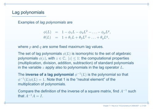
Lag polynomials
Examples of lag polynomials are
φ(L) = 1 − φ1L − φ2L 2 − . . . − φpL p ,
θ(L) = 1 + θ1L + θ2L 2 + . . . + θqL q ,
where p and q are some fixed maximum lag values.
The set of lag polynomials φ(L) is isomorphic to the set of algebraic
polynomials φ(z), with z ∈ C, |z| ≤ 1: the computational properties
(multiplication, division, addition, subtraction) of standard polynomials
in the variable z apply also to polynomials in the lag operator L.
The inverse of a lag polynomial φ −1 (L) is the polynomial so that
φ −1 (L)φ(L) = 1. Note that 1 is the “neutral element” of the
multiplication of polynomials.
Compare the definition of the inverse of a square matrix, find A −1 such
that A −1 A = I.
Chapter 7.1 Heij et al, TI Econometrics II 2006/2007 – p. 21/24