Hybridization of Multi-Objective Evolutionary Algorithms and Artificial ...

Hybridization of Multi-Objective Evolutionary Algorithms and Artificial
Neural Networks for Optimizing the Performance of Electrical Drives
Alexandru-Ciprian Zăvoianu a,c Gerd Bramerdorfer b,c Edwin Lughofer a Siegfried Silber b,c
Wolfgang Amrhein b,c Erich Peter Klement a,c
a Department of Knowledge-based Mathematical Systems/Fuzzy Logic Laboratory Linz-Hagenberg, Johannes Kepler University of Linz,
Austria
b Institute for Electrical Drives and Power Electronics, Johannes Kepler University of Linz, Austria
c ACCM, Austrian Center of Competence in Mechatronics, Linz, Austria
Abstract
Performance optimization of electrical drives implies a lot of degrees of freedom in the variation of design parameters, which in turn
makes the process overly complex and sometimes impossible to handle for classical analytical optimization approaches. This, and
the fact that multiple non-independent design parameter have to be optimized synchronously, makes a soft computing approach
based on multi-objective evolutionary algorithms (MOEAs) a feasible alternative. In this paper, we describe the application of
the well known Non-dominated Sorting Genetic Algorithm II (NSGA-II) in order to obtain high-quality Pareto-optimal solutions
for three optimization scenarios. The nature of these scenarios requires the usage of fitness evaluation functions that rely on very
time-intensive finite element (FE) simulations. The key and novel aspect of our optimization procedure is the on-the-fly automated
creation of highly accurate and stable surrogate fitness functions based on artificial neural networks (ANNs). We employ these
surrogate fitness functions in the middle and end parts of the NSGA-II run (→ hybridization) in order to significantly reduce
the very high computational effort required by the optimization process. The results show that by using this hybrid optimization
procedure, the computation time of a single optimization run can be reduced by 46% to 72% while achieving Pareto-optimal
solution sets with similar, or even slightly better, quality as those obtained when conducting NSGA-II runs that use FE simulations
over the whole run-time of the optimization process.
Key words: electrical drives, performance optimization, multi-objective evolutionary algorithms, feed-forward artificial neural networks,
surrogate fitness evaluation, hybridization
1. Introduction
1.1. Motivation
Today, electrical drives account for about 70% of the total
electrical energy consumption in industry and for about
40% of used global electricity [1]. In [2] it is stated that,
each year, in the European Union, the amount of wasted
energy that could be saved by increasing the efficiency of
electrical drives is around 200TWh and for this reason, in
2009, a European regulation was concluded forcing a gradual
increase of the energy efficiency of electrical drives [3].
However, manufacturers of electrical machines need to take
more than just the efficiency into account to hold their
own value in the global market. To be able to successfully
compete, the electrical drives should be fault-tolerant and
should offer easy to control operational characteristics and
compact dimensions. Apart from these, the most important
quality factor is the price. During the development of
an electrical machine, a multi-objective optimization approach
[4,5] is required in order to address all of the above
aspects and to find an appropriate tradeoff between the final
efficiency and the cost of the drive.
1.2. State-of-the-Art in Electrical Drive Design
In the past, electrical machines were designed by applying
a parameter sweep and calculating a maximum of
several hundred designs [6]. Calculating a design actually
means predicting the operational behavior of the electrical
drive for a concrete set of parameter settings. Because
of the nonlinear behavior of the materials involved, such
a prediction needs to be based on time intensive finite element
simulations. This, combined with the need to have
Preprint submitted to Engineering Application of Artificial Intelligence 1 July 2013

an acceptable duration of the overall analysis, imposed a
severe limitation in the number of designs to be calculated.
As such, only major design parameters could be taken into
consideration and only a rather coarse parameter step size
could be applied.
During the last decade, the use of response surface
methodology [7], genetic algorithms [8,9], particle swarm
optimization [10] and other techniques [11] for the design
of electrical machines and the associated electronics has
become state-of-the-art. For a detailed comparisons of
these modern approaches and additional reviews of the
state-of-the-art in electrical drive design, the reader is
kindly directed to consult [12–14].
Although the above mentioned search methods have
proved to be far more suitable for the task of multiobjective
optimization than basic parameter sweeps, they
are still plagued by the huge execution times incurred
by the need to rely on FE simulations throughout the
optimization procedure. The usage of computer clusters
where multiple FE simulations can be performed in parallel
can partially address this problem, but the following
drawbacks still remain severe:
– The FE evaluation of one particular design still takes
a long time and conventional methods need to evaluate
each individual design.
– There are high costs associated with the usage of computer
clustering architectures and various software licenses.
1.3. Our Approach
In our attempt to create an efficient optimization framework
for electrical drive design, we are exploiting well
known and widely applied genetic algorithms used for
multi-objective optimization. These specialized algorithms
are generally able to efficiently handle several optimization
objectives. For us, these objectives are electrical drive
target parameters like efficiency, cogging torque, total iron
losses, etc. In our implementation, the goal is to minimize
all the objectives. If a target needs to be maximized in the
design (e.g., efficiency), during the optimization, its negative
value is taken to be minimized. The FE simulations
required by each fitness function evaluation are distributed
over a high throughput computer cluster system. Although
it is able to evolve electrical drive designs of remarkable
high quality, the major drawback of this initial, and somewhat
conventional, optimization approach (ConvOpt)
is that it is quite slow as it exhibits overall optimization
run-times that vary from ≈ 44 to ≈ 70 hours. As a particular
multi-objective genetic algorithm, we employ the
well-known and widely used NSGA-II[15].
One main method aimed at improving the computational
time of a multi-objective evolutionary algorithm that has
a very time-intensive fitness function is to approximate the
actual function through means of metamodels / surrogate
models [16]. These surrogate models can provide a very
2
accurate estimation of the original fitness function at a
fraction of the computational effort required by the latter.
Three very well documented overviews on surrogate based
analysis and optimization can be found in [17], [18] and [19].
In our case, the idea is to substitute the time-intensive
fitness functions based on FE simulations with very-fastto-evaluate
surrogates based on highly accurate regression
models. The surrogate models act as direct mappings between
the design parameters (inputs) and the electric drive
target values which should be estimated (outputs). For us,
in order to be effective in their role to reduce overall optimization
run-time, the surrogate models need to be constructed
on-the-fly, automatically, during the run of the
evolutionary algorithm. This is because they are quite specific
for each optimization scenario and each target value
(i.e., optimization goal or optimization constraint) that we
consider.
In other words, we would like that only individuals (i.e.,
electrical drive designs) from the first N generations will
be evaluated with the time-intensive FE-based fitness function.
These initial, FE evaluated, electrical drive designs
will form a training set for constructing the surrogate models.
For the remaining generations, the surrogate models
will substitute the FE simulations as the basis of the fitness
function. As our tests show, this yields a significant
reduction in computation time.
The novelty of our research lies in the analysis of how
to efficiently integrate automatically created on-the-flysurrogate-models
in order to reduce the overall optimization
run-time without impacting the high quality of the
electrical drive designs produced by ConvOpt.
Artificial Neural Networks (ANNs) [20] are among the
popular methods used for constructing surrogate models
because they possess the universal approximation capability
[21] and they offer parameterization options that allow
for an adequate degree of control over the complexity of
the resulting model. Another advantage of ANNs is the fact
that they are known to perform well on non-linear and noisy
data [22] and that they have already been successfully applied
in evolutionary computation for designing surrogate
models on several instances [23,24]. For the purpose of this
research, the particular type of ANN we have chosen to use
is the multilayered perceptron (MLP). MLP is a popular
and widely used neural network paradigm that has been
successfully employed to create robust and compact prediction
models in many practical applications [25,26]. However,
our choice for the MLP is first and foremost motivated
by the fact that, for our specific modeling requirements,
MLP-bases surrogate models have proved to be both relatively
fast and easy to create as well as extremely accurate.
There is a wide choice of methods available for constructing
surrogate models. In this paper, we describe in details
how we created surrogates based on MLPs, but our hybridization
schema itself is general and suitable for a multitude
of modeling methods. In Section 5.1 we present results
obtained with other non-linear modeling methods that can
be used as alternatives for constructing the surrogate mod-

els. These modeling methods are, support vector regression
(SVR) [27], RBF networks [28] and a regression orientated
adaptation of the instance based learning algorithm IBk
[29]. In the aforementioned section, we also further motivate
our current preference for MLP surrogate models.
Regardless of the modeling method used, the automatic
surrogate model construction phase involves testing different
parameter settings (e.g. different number of neurons
and learning rates in the case of MLPs, different values of C
and γ in the case of SVR), yielding many models with different
complexities and prediction behaviors. Given a certain
target parameter we propose a new, automated model
selection criterion, aimed at selecting the best surrogate
to be integrated in the optimization process. The selected
surrogate model should deliver the best tradeoff between
smoothness, accuracy and sensitivity, i.e., the lowest possible
complexity with an above-average predictive quality.
The rest of this paper is organized in the following way:
Section 2 presents an overview of multi-objective optimization
problems (MOOPs) in general with a special focus
on the particular complexities associated with MOOPs encountered
in the design and prototyping of electrical drives.
Section 3 contains a description of our hybrid optimization
procedure (HybridOpt) focusing on the creation and integration
of the MLP surrogate models. Section 4 provides
the description of the experimental setup. Section 5 contains
an evaluation of the performance of the hybrid optimization
process with regards to the overall run-time of
the simulations and the quality of the obtained solutions.
Section 6 concludes the paper with a summary of achieved
and open issues.
2. Problem Statement
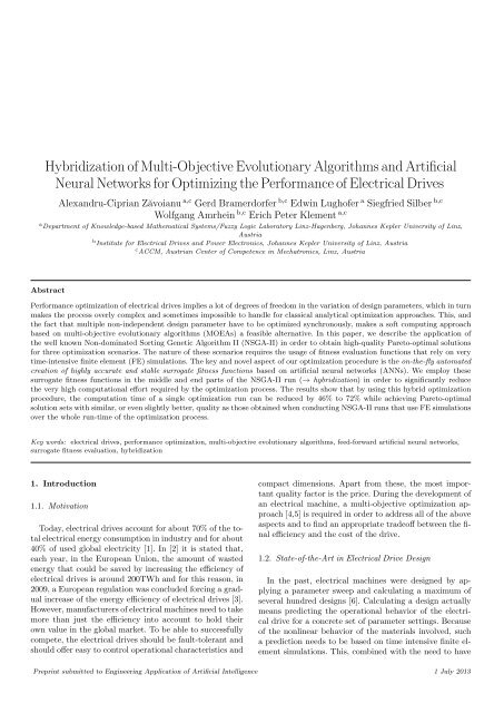
The design of an electrical machine usually comprises at
least the optimization of geometric dimensions for a preselected
topology. Figure 1 gives the cross-section of an
electrical drive featuring a slotted stator with concentrated
coils and an interior rotor with buried permanent magnets.
The geometric parameters of this assembly are depicted in
the figure (dsi, bst, bss. etc.). Depending on the actual problem
setting, usually, most of these parameters need to be
varied in order to achieve a cheap motor with good operational
behavior. Furthermore, due to the fast moving
global raw material market, companies tend to investigate
the quality of target parameters with regard to different
materials. Sometimes, the study of different topologies is
also required during the design stage. All these lead to a
relatively high number of input parameters for the optimization
procedure.
Furthermore, because the behavior of the materials used
to construct the electrical drive cannot be modeled linearly,
the evaluation of a given design has to be done by using
computationally expensive FE simulations. These are solving
non-linear differential equations in order to obtain the
values of the target parameters associated with the actual
3
(a) Stator
(b) Rotor
Fig. 1. Geometric dimensions of the stator and rotor for an interior
rotor topology with embedded magnets
design parameter vector. Specifically, we use the software
package FEMAG TM [30] for the calculation of 2D problems
on electro-magnetics.
As our main goal is the simultaneous minimization of all
the objectives (target values) involved, we are faced with
a multi-objective optimization problem which can be formally
defined by:
where
min (o1(X), o2(X), ..., ok(X)), (1)
o1(X), o2(X), ..., ok(X) (2)
are the objectives (i.e. target parameters) that we consider
and
X T
= x1 x2 . . . xn
(3)
is the design parameter vector (e.g. motor typology identifier,
geometric dimensions, material properties, etc).

Additionally, hard constraints like (4) can be specified
in order to make sure that the drive exhibits a valid operational
behavior (e.g. the torque ripple is upper bound).
Such constraints are also used for invalidating designs with
a very high price.
c(x) ≤ 0 ∈ R m
In order to characterize the solution of MOOPs it is helpful
to first explain the notion of Pareto dominance [31]:
Definition 1 Given a set of objectives, a solution A is said
to Pareto dominate another solution B if A is not inferior
to B with regards to any objectives and there is at least one
objective for which A is better than B.
The result of an optimization process for a MOOP is
usually a set of Pareto-optimal solutions named the Pareto
front [31] (a set where no solution is Pareto dominated by
any other solution in the set). The ideal result of the multiobjective
optimization is a Pareto front which is evenly
spread and situated as close as possible to the true Pareto
front of the problem (i.e., the set of all non-dominated solutions
in the search space).
3. Optimization Procedure
3.1. Conventional Optimization using Multi-Objective
Evolutionary Algorithms
As most evolutionary algorithms (EAs) work generationwise
for improving sets (populations) of solutions, various
extensions aimed at making EA populations store and efficiently
explore Pareto fronts have enabled these types of
algorithms to efficiently find multiple Pareto-optimal solutions
for MOOPs in one single run. Such algorithms are
referred to as multi-objective evolutionary algorithms or
MOEAs in short.
In our case, each individual from the MOEA population
will be represented as a fixed length real parameter vector
that is actually an instance of the design parameter vector
described in (3). Computing the fitness of every such
individual means computing the objective functions from
(2) and, at first, this can only be achieved by running FE
simulations.
The Non-dominated Sorting Genetic Algorithm II
(NSGA-II) [15] proposed by K. Deb in 2002 is, alongside
with the Strength Pareto Evolutionary Algorithm 2
(SPEA2) [32], one of the most successful and widely applied
MOEA algorithms in literature. A brief description of
NSGA-II is presented in Appendix A. On a close review, it
is easy to observe that both mentioned MOEAs are based
on the same two major design principles:
(i) an elitist approach to evolution implemented using a
secondary (archiving) population;
(ii) a two-tier selection for survival function that uses
a primary Pareto non-dominance metric and a secondary
density estimation metric;
(4)
4
In light of the above, it is not surprising that the respective
performance of these two algorithms is also quite similar
[32,33] with minor advantages towards either of the two
methods depending on the particularities of the concrete
MOOP problem to be solved [34,35]. Taking into account
the similarity of the two MOEAs and the very long execution
time required by a single optimization run, we mention
that all the tests reported on over the course of this research
have been carried out using NSGA-II. Our choice for
this method is also motivated by a few initial comparative
runs in which the inherent ability of NSGA-II to amplify
the search around the extreme Pareto front points enabled
it to find a higher number of very interesting solutions than
SPEA2 for two of our optimization scenarios.
3.2. Hybrid Optimization using a Fitness Function based
on Surrogate Models
3.2.1. Basic Idea
Our main approach to further improve the run time
of the our optimization process is centered on substituting
the original FE-based fitness function of the MOEAs
with a fitness function based on surrogate models. The
main challenge lies in the fact that these surrogate models,
which must be highly accurate, are scenario dependent
and as such, for any previously unknown optimization
scenario, they need to be constructed on-the-fly (i.e.,
during the run of the MOEA). A sketch of the surrogatebased
enhanced optimization process (HybridOpt) outlining
the several new stages it contains in order to incorporate
surrogate-based fitness evaluation is presented in Figure 2.
In the FE-based MOEA execution stage the first N generations
of each MOEA run are computed using FE simulations
and all the individuals evaluated at this stage will
form the training set used to construct the surrogate models.
Each sample in this training set contains the initial
electrical motor design parameter values (3) and the corresponding
objective function values (2) computed using
FEMAG TM . Please refer to Section 5.2 for a description
of the methodology we used in order to determine a good
value of N.
In the surrogate model construction stage, we use systematic
parameter variation and a selection process that takes
into consideration both accuracy and architectural simplicity
to find and train the most robust surrogate design for
each of the considered target variables.
The next step is to switch the MOEA to a surrogatebased
fitness function for the remaining generations that we
wish to compute (surrogate-based MOEA execution stage).
The surrogate-based fitness function is extremely fast when
compared to its FE-based counterpart, and it enables the
prediction of target values based on input variables within
milliseconds. Apart from improving the total run time of
the MOEA simulation, we can also take advantage of this
massive improvement in speed in two other ways:
(i) by increasing the total number of generations the

Fig. 2. Diagram of the conventional optimization process - ConvOpt and of the surrogate-enhanced optimization process - HybridOpt when
wishing to compute a total of M generations
MOEA will compute during the simulation;
(ii) by increasing the sizes of the populations with which
the MOEA operates;
Both options are extremely important as they generally
enable MOEAs to evolve Pareto fronts that are larger in
size and exhibit a better spread.
In the surrogate-based Pareto front computation stage
a preliminary surrogate-based Pareto front is extracted
only from the combined set of individuals evaluated using
the surrogate models. This secondary Pareto front is constructed
independently, i.e., without taking into consideration
the quality of the FE-evaluated individuals in the first
N generations. Initial tests have shown that this approach
makes the surrogate-based front less prone to instabilities
induced by inherent prediction errors and by the relative
differences between the qualities of the surrogate models.
We mention that, in the current stage of development,
at the end of the MOEA run (the FE-based reevaluation
stage), it is desired that all the Pareto-optimal solutions
found using the surrogate models are re-evaluated using FE
calculations. There are two main reasons for which we do
this. The first one is a consequence of the fact that in our
optimization framework, the check for geometry errors is
tightly coupled with the FE evaluation stage and as such
some of the Pareto optimal solutions found using the surrogate
models might actually be geometrically invalid. The
second reason for the re-evaluation is to assure that all the
simulation solutions presented as Pareto optimal have the
same approximation error (i.e., the internal estimation error
of the FEMAG TM software).
In the final Pareto front computation stage, the final
Pareto front of the simulation is extracted from the combined
set of all the individuals evaluated using FE simula-
5
tions, i.e., individuals from the initial N generations and
FE-reevaluated surrogate-based individuals.
It is important to note that our enhanced optimization
process basically redefines the role of the FE simulations.
These very accurate but extremely time intensive
operations are now used at the beginning of the MOEA
driven optimization process, when, generally, the qualityimprovement
over computation time ratio is the highest.
FE simulations are also used in the final stage of the optimization
process for analyzing only the most promising
individuals found using the surrogate models. In the middle
and in the last part of the optimization run, when
quality improvements would come at a much higher computational
cost, a surrogate-based fitness function is used
to steer the evolutionary algorithm.
In the results section, we will show that, using the surrogate
enhancement, Pareto fronts with similar quality to
the ones produced by ConvOpt can be obtained while significantly
reducing the overall simulation time.
3.2.2. The Structure and Training of ANN Surrogate
Models
Generally, the MLP architecture (Figure 3) consists of
one layer of input units (nodes), one layer of output units
and one or more intermediate (hidden) layers. MLPs implement
the feed-forward information flow which directs
data from the units in the input layer through the units
in the hidden layer to the unit(s) in the output layer. Any
connection between two units ui and uj has an associated
weight wij that represents the strength of that respective
connection. A concrete MLP prediction model is defined
by its specific architecture and by the values of the weights
between its units.

Given the unit ui, the set Pred(ui) contains all the units
uj that connect to node ui, i.e. all the units uj for which
wji exists. Similarly, the set Succ(ui) contains all the units
uk to which node ui connects to, i.e. for which wik exists.
Each unit ui in the network computes an output value
f(ui) based on a given set of inputs. Depending on how
this output is computed, one may distinguish between two
types of units in a MLP:
(i) Input units - all the units in the input layer. The role
of these units is to simply propagate into the network
the appropriate input values from the data sample we
wish to evaluate. In our case, f(ui) = xi where xi is
the i th variable of the design parameter vector from
(3).
(ii) Sigmoid units - all the units in the hidden and output
layers. These units first compute a weighted sum of
connections flowing into them (5) and then produce
an output using a non-linear logistic (sigmoid shaped)
activation function (6):
s(ui) =
uj∈Pred(ui)
wjif(uj) (5)
1
f(ui) = P (ui) =
1 + e−s(ui) (6)
In our modeling tasks, we use MLPs that are fully connected,
i.e. for every sigmoid unit ui, Pred ui exclusively
contains all the units in the previous layer of the network.
In the input layer, we use as many units as design variables
in the data sample. Also, as we construct a different surrogate
model for each target variable in the data sample,
the output layer contains just one unit and, at the end of
the feed-forward propagation, the output of this unit is the
predicted regression value of the elicited target (e.g. P (o1)
for the MLP presented in Figure 3).
The weights of the MLP are initialized with small random
values and then are subsequently adjusted during a training
process. In this training process we use a training set T
and every instance (data sample) −→ s ∈ T contains both the
values of the varied design parameters (i.e., XT ) as well as
the FE-computed value of the elicited target variable (e.g.,
syF E is the FE estimated value of o2(X) from (2) when
o2(X) is the target for which we wish to construct a MLP
surrogate model):
−→ s = (x1, x2, . . . , xn, yF E) (7)
The quality of the predictions made by the MLP can be
evaluated by passing every instance from the training set
through the network and then computing a cumulative error
metric (i.e., the batch learning approach). When considering
the MLP architecture presented in Figure 3 and
the squared-error loss function, the cumulative error metric
over training set T is:
E( −→ w ) = 1
2
(syF E − P (o1(sxi, −→ w ))) 2 , i = 1, m (8)
−→ s ∈T
6
Fig. 3. Multilayer perceptron model with one hidden layer and one
output unit
The goal of the training process is to adjust the weights
such as to minimize this error metric. The standard approach
in the field of ANNs for solving this task is the backpropagation
algorithm [36] which is in essence a gradientbased
iterative method that shows how to gradually adjust
the weights in order to reduce the training error of the MLP.
First, at each iteration t, the error metric Et ( −→ w ) is computed
using (8). Afterwards, each weight wt ij in the MLP
will be updated according to the following formulas:
∆w t ij = ηδ(uj)P (ui)
w t ij = w t ij + ∆w t ij if t = 1
w t ij = w t ij + ∆w t ij + α∆w t−1
ij
if t > 1
where η ∈ (0, 1] is a constant called the learning rate. By
α ∈ [0, 1), we mark the control parameter of the empirical
enhancement known as momentum, which can help the
gradient method to converge faster and to avoid some local
minima. The function δ(uj) shows the cumulated impact
that the weighted inputs coming into node uj have on
E t ( −→ w ) and is computed as:
(9)
δ(uj) = P (uj)(1 − P (uj))(y − P (uj)) (10)
if uj is the output unit and as:
δ(uj) = P (uj)(1 − P (uj))
uk∈Succ(uj)
δuk wjk
(11)
if uj is a hidden unit. The standard backpropagation
method proposes several stopping criteria: the number of
iterations exceeds a certain limit, E t ( −→ w ) becomes smaller
than a predefined ɛ, the overall computation time exceeds a
certain pre-defined threshold. We have chosen to adopt an
early stopping mechanism that terminates the execution
whenever the prediction error computed over a validation

subset V does not improve over 200 consecutive iterations.
This validation subset is constructed at the beginning of
the training process by randomly sampling 20% of the
instances from the training set T . This stopping criterion
may have a benefit in helping to prevent the overfitting of
MLP surrogate models.
3.2.3. The Evaluation and Automatic Model Selection of
ANN Surrogate Models
Usually, in MLP-based data modeling tasks the most important
design decision concerns the network architecture:
how many hidden layers to use and how many units to place
in each hidden layer. In order to construct a highly accurate
model, based on the previous architecture choice, one
should also experiment with several values for the learning
rate and momentum constants. In practice, this problem
is most often solved by experimentation usually combined
with some sort of expert knowledge.
It has been shown that MLPs with two hidden layers
can approximate any arbitrary function with arbitrary accuracy
[37] and that any bounded continuous function can
be approximated by a MLP with a single hidden layer and
a finite number of hidden sigmoid units [38]. The optimization
scenarios used in this research (see Section 4.1) do not
require the use of two hidden layers. Like with many other
interpolation methods, the quality of the MLP approximation
is dependent on the number of training samples that
are available and on how well they cover the input space. In
our application, we have the flexibility to select the number
of samples used for training the surrogate model according
to the complexity of the learning problem (i.e., number of
design parameters and their associated range values) and
this aspect is detailed in Section 5.2.
In order to automatically determine the number of hidden
units, the learning rate (η) and the momentum (α)
needed to construct the most robust MLP surrogate model,
we conduct a best parameter grid search, iterating over different
parameter value combinations (see Section 4.2 for
exact settings).
Our model selection strategy is aimed at finding the most
accurate and robust surrogate model where, by robust, we
understand a model that displays a rather low complexity
and a stable predictive behavior. Our tests have shown
that these two qualities are very important when striving
to construct surrogate models that enable the MOEAs to
successfully explore the entire search space.
The surrogate model selection process (Figure 4) is divided
in two stages. In the first stage, all the surrogates
are ranked according to a metric that takes into account
the accuracy of their predictions. Next, an accuracy threshold
is computed as the mean of the accuracies of the best
performing 2% of all surrogate models. The choice of the
final surrogate model is made using a complexity metric
that favors the least complex model that has a prediction
accuracy higher than the accuracy threshold. The general
idea is similar to that of a model selection strategy used for
7
Fig. 4. Diagram of the surrogate model selection process where the
predictive accuracy of the model is computed according to (12)
regression trees [39] with the noticeable difference that we
compute the accuracy threshold using a broader model basis
in order to increase stability (i.e., avoid the cases where
the accuracy threshold is solely set according to a highly
complex, and possibly overfit, model that is only marginally
more accurate than several much simpler ones).
The metric used to evaluate the prediction accuracy of
a surrogate model qm, is based on the coefficient of determination
(R 2 ). In order to evaluate the accuracy of a MLP
surrogate model we use a 10-fold cross-validation data partitioning
strategy [40] and we compute the value of R 2 over
each of the ten folds. The final accuracy assigned to the surrogate
model is the mean value of R 2 minus the standard
deviation of R 2 over the folds:
qm = µ(R 2 ) − σ(R 2 ) (12)
Using the standard deviation of R 2 over the cross-validation
folds as a penalty in (12) has the role of favoring models
that exhibit a more stable predictive behavior. The reason
for this is that a significant value of σ(R 2 ) indicates
that the surrogate model is biased toward specific regions
of the search space. The existence of locally-biased surrogate
models is quite probable because our training data is
rather unbalanced as it is the byproduct of a highly elitist
evolutionary process that disregards unfit individuals.
The second metric used in the surrogate model selection
process favours choosing less complex models. One MLP
surrogate model is considered to be more complex than
another if the former has more units in the hidden layer
(ties are broken in favor of the model that required more
computation time to train).
It is worth mentioning that this automatic surrogate
model selection strategy can easily be adapted when opting
for another surrogate modeling method. In this case,
one only needs to choose a different indicator (or set of indicators)
for measuring complexity (e.g. the C parameter
and/or the number of required support vectors in the case
of a SVR).

Algorithm 1 Description of the hybrid optimization process
1: procedure HybridOpt(Scenario, P opSizeini, P opSizeext, N, M)
2: P ← RandomlyInitializePopulation(Scenario, P opSizeini)
3: E ≡ FE-Evaluator(Scenario)
4: 〈P, V alidF E〉 ← NSGA-II-Search(N, P opSizeini, P, E)
5: Configurations ← InitializeMlpGridSearchConfigurations
6: for all target ∈ Scenario do
7: Map ← ∅
8: for all c ∈ Configurations do
9: Map ← Map∪ ConstructSurrogateModel(c, target, V alidF E)
10: end for
11: BestSurrogateModels(target) ← SelectBestSurrogateModel(Map)
12: end for
13: E ≡ SurrogateEvaluator(Scenario, BestSurrogateModels)
14: 〈P, V alidMLP 〉 ← NSGA-II-Search(M − N, P opSizeext, P, E)
15: OptimalSetMLP ← ExtractParetoFront(V alidMLP )
16: E ≡ FE-Evaluator(Scenario)
17: OptimalSetMLP ← EvaluateFitness(OptimalSetMLP , E)
18: return ExtractParetoFront(V alidF E ∩ OptimalSetMLP )
19: end procedure
20: function NSGA-II-Search(NrGen, P opSize, InitialP opulation, F itnessEvaluator)
21: t ← 1
22: V alidIndividuals ← ∅
23: P (t) ← InitialP opulation
24: P (t) ← EvaluateFitness(P (t), F itnessEvaluator)
25: while t ≤ NrGen do
26: O(t) ← CreateOffspring(P (t), P opSize)
27: O(t) ← EvaluateFitness(O(t), F itnessEvaluator)
28: V alidIndividuals ← V alidIndividuals ∪ O(t)
29: P (t + 1) ← ComputeNextPopulation(P (t), O(t), P opSize)
30: t ← t + 1
31: end while
32: return 〈P (t), V alidIndividuals〉
33: end function
3.2.4. Algorithmic Description of HybridOpt
Our hybrid optimization procedure is presented in Algorithm
1. Apart from method calls and the normal assignment
operator (←), we also use the operator ≡ in order to
mark the dynamic binding of a given object to a specific
method with the implied meaning that all future references
to the object are redirected to the corresponding targeted
method.
The main procedure, named HybridOpt, has five input
parameters:
– Scenario - the description of the scenario to be optimized
with information regarding design parameters and targets
– P opSizeini - the size of the NSGA-II population for the
FE-based part of the run
– P opSizeext - the size of the NSGA-II population for the
surrogate-based part of the run
– N - the number of generations to be computed in the
FE-based part of the run
– M - the total number of generations to be computed
8
during the optimization (i.e., M − N generations will be
computed in the surrogate-based part)
The NSGA-II implementation contained in the NSGA-
II-Search function differs from standard implementations
as it returns two results, the Pareto optimal set obtained
after constructing the last generation and a set containing
all the valid individuals generated during the search. This
function has four input parameters:
– NrGen - the number of generations to be computed
– P opSize - the size of the population
– InitialP opulation - a set containing the starting population
of the evolutionary search
– F itnessEvaluator - an object that is bound to a specific
fitness evaluation function
The method EvaluateFitness is of particular importance.
It receives as input a set of unevaluated individuals
and an object that is bound to a specific fitness evaluation
function. EvaluateFitness returns a filtered set containing
only the valid individuals. Each individual in the returned
set also stores information regarding its fitness over

the multiple objectives — note that the fitness is directly
associated with the values of the target parameters, which
are either predicted by the surrogate model or calculated
using differential equations in the FE simulation. If the concrete
fitness function used is FE-Evaluator, individuals
are checked for validity with regards to both geometrical
(meshing) errors and constraint satisfaction (4). Geometrical
errors may arise because of specific combinations of
design parameter values. When using the SurrogateEvaluator,
only constraint satisfaction validity checks can
be performed.
The other methods that we use in HybridOpt are:
– RandomlyInitializePopulation - this method randomly
initializes a set of individuals of a given size according
to the requirements of the optimization scenario
to be solved
– InitializeMlpGridSearchConfigurations - this
method constructs all the MLP training configurations
that are to be tested in a best parameter grid search (see
Section 4.2 for details)
– ConstructSurrogateModel - this method builds a
single MLP surrogate model for a given target based on
a preset MLP training configuration and a training set
of previously FE-evaluated individuals as described in
Section 3.2.2
– SelectBestSurrogateModel - this method selects
the most robust surrogate from a given set of models
according to the surrogate model selection process described
in Section 3.2.3
– ExtractParetoFront - this method extracts the
Pareto-optimal front from a given set of possible solutions
after the description in Section 3.1.
In the NSGA-II-Search method, the functions CreateOffspring
and ComputeNextPopulation are responsible
for implementing the evolutionary mechanism described
in Appendix A.
4. Experimental Setup
4.1. The Optimization Scenarios
We consider three multi-objective optimization scenarios
coming from the field of designing and prototyping electrical
drives:
The first scenario (Scenario OptS1 ) is on a motor for
which the rotor and stator topologies are shown in Figure
1. The design parameter vector has a size of six and is given
by
X T
=
,
hm αm er dsi bst bss
where all parameters are illustrated in Fig. 1 except for
αm, which denotes the ratio between the actual magnet
size and the maximum possible magnet size as a result of
all other geometric parameters of the rotor. The targets for
the MLP surrogate model construction stage are the four,
unconstrained, Pareto objectives:
9
– T 1 = −η - where η denotes the efficiency of the motor. In
order to minimize the losses of the motor, the efficiency
should be maximized and therefore −η is selected for
minimization.
– T 2 = TcogP P - the peak-to-peak-value of the motor
torque for no current excitation. This parameter denotes
the behavior of the motor at no-load operation
and should be as small as possible in order to minimize
vibrations and noise due to torque fluctuations.
– T 3 = T otalCosts- the material costs associated with a
particular motor. Obviously, minimizing this objective is
a very important task in most optimization scenarios.
– T 4 = TrippP P - the equivalent of Tcog,P P at load operation.
The values of this objective should also be as small
as possible.
The second problem (Scenario OptS2 ) is on an electrical
machine featuring an exterior rotor. The design parameter
vector contains seven geometric dimensions. The aim of
this optimization problem was to minimize the total losses
of the system at load operation and to minimize the total
mass of the assembly while simultaneously maintaining
other desired operational characteristics (e.q., efficiency,
cogging torque, costs, etc). In the case of this scenario, the
first target (T 1) is a hard-constrained Pareto optimization
goal, the second (T 2) is an unconstrained Pareto optimization
goal, whilst the third (T 3) is a secondary hard constraint
imposed on the evolved motor designs.
The third problem (Scenario OptS3 ) also concerns a motor
with an exterior rotor. The design parameter vector has
a size of ten. This scenario proposes four, hard-constrained,
Pareto optimization goals. All of them are considered targets
in the surrogate model construction phase:
– T 1 = ls - the total axial length of the assembly
– T 2 = T otalMass - the total mass of the assembly
– T 3 = PCu- the ohmic losses in the stator coils
– T 4 = Pfe - the total losses due to material hysteresis and
eddy currents in the ferromagnetic parts of the motor
4.2. The Testing Framework
In order to compare the performance of the two optimization
processes we are using optimization runs that compute
100 generations with a population size of 50. This rather
small choice of the population size is motivated by restrictions
regarding time and the available cluster computation
power for running the required simulations.
In order to illustrate some immediate benefits of using
the enhanced approach (see Section 3.2.1), we also performed
tests where, during the run of the MOEA, after the
construction of the mappings, we doubled the population
size and the number of generations to be evolved.
Our optimization framework uses the NSGA-II implementation
provided by the jMetal package [41]. For all tests
reported in Section 5, we used NSGA-II with a crossover
probability of 0.9, a crossover distribution index of 20, a
mutation probability of 1/|X T | and a mutation distribu-

tion index of 20. The high values of the distribution indexes
for the crossover and mutation operators (that are
recommended by literature [15] and set as default in jMetal)
force NSGA-II to generate near parent values for almost all
spawned offspring. While this parameter choice seems to
determine an overall search strategy that favors exploitation
over exploration, the highly elitist nature of NSGA-II
coupled with the high mutation probability, help to balance
the exploitation versus exploration ratio over the entire
run. Using ConvOpt, we have performed a tuning phase
to check whether smaller values (i.e., 15, 10, 5 and 2) for
the crossover and mutation distribution indexes would yield
better results when using a population size of 50 and a
limited number of evolved generations. The results showed
that using these smaller index values does not produce any
improvement.
In the case of HybridOpt, we perform the mapping training
stage after N = 25 generations (please see Section 5.2
for a detailed explanation of this parameter choice). As we
use a population size of 50, the maximum possible size of
the training sets is 1250 samples. The size of the actual
training sets we obtained was smaller because some of the
evolved design configurations were geometrically unfeasible
or invalid with regards to given optimization constraints.
When considering all the performed tests, the average sizes
and standard deviations of the obtained training sets is presented
in Table 1.
Table 1
The average size and standard deviations of the obtained training
sets.
Scenario Training set size µ Training set size σ
OptS1 1219.50 22.40
OptS2 813 123.59
OptS3 743.25 74.33
The MLP implementation we used for our tests is largely
based on the one provided by the WEKA open source machine
learning platform [42]. In the case of the best parameter
grid searches that we performed in order to create the
MLP surrogate models:
– the number of hidden units was varied between 2 and
double the number of design variables;
– η was varied between 0.05 and 0.40 with a step of 0.05
– α was varied between 0.0 and 0.7 with a step of 0.1
The search is quite fine grained as it involves building
between 704 (scenario OptS1 ) and 1216 (scenario OptS3 )
MLP surrogate models for each elicited target. This approach
is possible because we make use of the early stopping
mechanism in the MLP training process (see Section 3.2.2)
which in turn ensures an average surrogate model training
time of 356.70 seconds. We achieve a considerable speedup
in the surrogate model creation stage by distributing all the
MLP training tasks over the same high throughput cluster
computing environment that is used to run in parallel the
FE simulations. As a result, the surrogate model creation
10
stage took, on average, 146.33 minutes, over all performed
tests.
4.3. Considered Performance Metrics
In order to compare the performance and behavior of the
conventional and hybrid optimization processes we use four
performance metrics:
(i) the hypervolume metric H [43] measures the overall
coverage of the obtained Pareto set;
(ii) the generalized spread metric S [44] measures the relative
spatial distribution of the non-dominated solutions;
(iii) the FE utility metric U offers some insight on the
efficient usage of the FE evaluations throughout the
optimization;
(iv) the run-time metric T records the total runtime in
minutes required by one optimization;
The hypervolume and generalized spread metrics are
commonly used in MOEA literature when comparing between
different non-dominated solution sets. The H metric
has the added advantage that it is the only MOEA metric
for which we have theoretical proof [45] of a monotonic
behavior. This means that the maximization of the hypervolume
constitutes the necessary and sufficient condition
for the set of solutions to be “maximally diverse Pareto
optimal solutions of a discrete, multi-objective, optimization
problem”. By design, the upper bound of H is 1.00.
For any optimization problem, the true Pareto front yields
the highest H value. As we are not dealing with artificial
problems, for our considered scenarios, the best possible
value of H for each problem is unknown.
In the case of the S metric, a value closer to 0.0 indicates
that the solutions are evenly distributed in the search
space. Although this metric is not monotonic in showing
true Pareto front convergence, in our case, it is extremely
useful as it is a good indicator of the diversity of Paretooptimal
electrical drive designs that our optimization runs
are able to find.
The FE utility metric is constructed for the purpose of
illustrating how efficiently the optimization process is using
the very time intensive FE simulations over an entire
run. The U metric is computed as the ratio between the
total number of non-dominated solutions found during the
optimization (i.e. the size of the final Pareto front) and the
total number of performed FE simulations.
5. Results
5.1. Overview of MLP Surrogate Model Performance
In order to offer a quick insight into the characteristics of
the elicited target variables, Table 3 contains the comparative
results of trying to model the targets using linear regression,
MLPs and three other non-linear modeling methods.
We considered sets containing all the samples obtained

(a) Scenario OptS1
(b) Scenario OptS2
(c) Scenario OptS3
Fig. 5. Evolution of the coefficient of determination computed over
the remaining 100−n generations for the best MLP surrogate models
trained using the first n ≤ 50 generations
using FE simulations over 100 NSGA-II generations with a
population size of 50 and split them into training and test
data sets. The training data sets contain the individuals
from the first 33 generations while the test data sets are
made up from the individuals from the last 67 generations
(i.e., a ”1/3 - training , 2/3 - test” data set partitioning
scheme). After removing the geometrically unfeasible and
invalid designs, we ended up with training sets of size 1595
(OptS1 ), 1197 (OptS2 ), and 1103 (OptS3 ).
For the non-linear modeling methods, we report the test
result achieved by the best surrogate model which was se-
11
lected based on 10-fold cross-validation performance after
doing a best parameter grid search on the training data.
In the case of the MLP, the grid search was set up as described
in Section 4.2. In the case of SVR, we trained 675
surrogate models for each target as we varied: the general
complexity parameter C between [2 −4 , 2 −3 , ..., 2 10 ],
the RBF kernel parameter γ between [2 −5 , 2 −4 , ..., 2 3 ]
and the ɛ parameter of the ɛ-intensive loss function between
[0.001, 0.005, 0.01, 0.025, 0.05]. For RBF networks,
we trained 918 surrogate models for each target by varying
the number of clusters between [2, 3, 4, 5, 10, 20, ..., 500]
and the allowed minimum standard deviation for the clusters
between [0.25, 0.5, 1.00, 2.00, ...15.0]. When using IBk
modeling, we created 900 surrogate models for each target
as we varied the number of nearest neighbors from 1 to 300
and we used three different distance weighting options: no
weighting, weight by 1/distance and weight by 1-distance.
Firstly, one can observe that while most targets display
a strong linear dependency towards their respective
design variables, the surrogate models obtained using linear
regression for some targets (e.g., OptS1-T1, OptS1-T2,
OptS1-T4, OptS3-T4 ) are by no means accurate. For the
purpose of this research, we decided on a linear regression
R 2 threshold value of 0.9 in order to classify a target as
linear or non-linear.
When considering only the six non-linear targets, MLPs
and SVR are the best performers (MLP slightly better than
SVR) while RBF networks produce results that are significantly
worse. We conducted all the best parameter grid
searches by distributing the surrogate model training tasks
over the computer cluster. We measured the time required
by the grid searches conducted for non-linear targets and,
for each modeling method, averaged it over the total number
of surrogate models to be trained. We present these results
in Table 2 and, together with some model complexity
information, they indicate that, when comparing with the
MLP:
– RBF networks and SVR require ≈ 15% and ≈ 55% more
(wall) time in order to finish the grid search.
– when taking into acount the sizes of the training sets,
RBF networks and SVR seem to produce surrogate models
that are quite complex (i.e., number of clusters required
by the RBF network and number of support vectors
used by SVR)
The difference in required training time, the low structural
complexity, and the higher accuracy motivate our
choice of using MLP surrogate models.
5.2. The Accuracy and Stability of MLP Surrogate Model
Predictions
In the current version of HybridOpt, it is very important
to choose a good value for the parameter N that indicates
for how many generations we wish to run the initial FEbased
execution stage. A value of the parameter that is too
low will result in creating inconclusive training sets which

Table 2
Information regarding the average training time of the surrogate models and the structural complexity (i.e., number of hidden units in the
case of MLP, number of support vectors in the case of SVR and number of clusters in the case of RBF networks) of the best surrogate model
on the non-linear targets
Target
OptS1-T1
Average training time [minutes] Complexity indicator of the best surrogate
MLP SVR RBF Nets MLP SVR RBF Nets
11 892 500
OptS1-T2 0.734 1.241 0.865 12 754 500
OptS1-T4 11 1046 500
OptS2-T1 0.678 0.931 0.620 9 323 300
OptS3-T3
0.601 0.945 0.837
12 858 400
OptS3-T4 10 868 400
All non-linear 0.671 1.039 0.774 10.83 790.16 433.33
Table 3
Linear and non-linear regression modeling results on the elicited targets
Scenario Target Classification
OptS1
OptS2
OptS3
R 2 on test instances
Linear MLP SVR RBF Nets IBk
T1 non-linear 0.7353 0.9864 0.9330 0.9029 0.8744
T2 non-linear 0.6048 0.9530 0.9540 0.8992 0.9040
T3 linear 0.9777 0.9992 0.9997 0.9999 0.9660
T4 non-linear 0.6390 0.9674 0.9640 0.9099 0.9044
T1 non-linear 0.8548 0.9923 0.9960 0.9859 0.9749
T2 linear 0.9916 0.9997 0.9997 0.9998 0.9904
T3 linear 0.9990 0.9999 0.9998 0.9999 0.9254
T1 linear 0.9970 0.9999 0.9997 0.9999 0.9689
T2 linear 0.9514 0.9998 0.9995 0.9999 0.8822
T3 non-linear 0.8526 0.9799 0.9839 0.9804 0.8791
T4 non-linear 0.8355 0.9564 0.9552 0.9521 0.8794
Average All linear 0.9830 0.9997 0.9997 0.9997 0.9466
Average All non-linear 0.7540 0.9720 0.9640 0.9384 0.9026
Average All all 0.8580 0.9847 0.9802 0.9664 0.9226
in turn will lead to surrogate models that are not globally
accurate or stable. By choosing a value for N that is a lot
higher than the optimal one, we are more or less ”wasting”
FE simulations by creating oversized training sets. In order
to choose a good value of N we take into account the influence
that this parameter has on the accuracy and stability
of the resulting MLP surrogate models.
In order to estimate the influence that N has on the accuracy
of the surrogate models, for each optimization scenario
we consider fully FE-based runs of 100 generations
and the combined pools of samples that each such simulation
produces. We construct 50 different test cases and, for
each target of each scenario, we divide the available samples
into a training and a test set. For test number i, the
training set contains the individuals from the first i generations
and the validation set contains the individuals from
the last 100 − i generations. For each test, we use the best
parameter grid search and the automated model selection
12
strategy in order to obtain the best MLP surrogate model
on the training data. Next, we evaluate the quality of this
surrogate model by computing the coefficient of determination
over the corresponding test set. The resulting values
are plotted in Figure 5. It can be easily observed that
all targets display a stable logarithmic saturation behavior
that suggests that a choice of N in the 20 to 30 generations
range should be able to produce highly accurate surrogate
models for all considered targets.
The concrete decision for the value of N is based on the
stability over time of the obtained surrogate models. We estimate
the stability over time by computing the individual
R 2 of every generation in the test data sets. For example,
Figure 6 contains the plots of the generational coefficients
of determination for the most difficult to model targets of
scenarios OptS1 and OptS3 (i.e., OptS1-T2 and OptS3-
T4 ). We are only interested in the best surrogate models
constructed using the samples from the first 20 to 30 gen-

(a) Target OptS1-T2
(b) Target OptS3-T4
Fig. 6. Evolution of the generational coefficient of determination for MLP surrogate models trained using the first 20 to 30 generations for
the most difficult to model targets
erations.
Finally, we have chosen N = 25 as this is the smallest
value of N for which the trained surrogate models exhibit
both a high prediction accuracy as well as a high prediction
stability. Over all three data sets and the 6 non-linear
targets, the generational coefficients of determination (for
generations 31 to 100) obtained by the surrogate models
constructed using samples from the first 25 generations:
– are higher than 0.9 in 94.52% of the cases;
– are higher than those obtained by the surrogate models
constructed using 20-24 generations in 57.52% of the
cases and by those obtained by the surrogate models constructed
using 26-30 generations in 42.52% of the cases;
All HybridOpt tests reported in the next section have
been performed with the parameter setting of N = 25.
5.3. The Comparative Performance of HybridOpt
In Table 4 we present the comparative performance of
ConvOpt and HybridOpt after runs of 100 generations
each. The results for each scenario are averaged over five
independent runs. For these tests, the size of the population
in HybridOpt was fixed, throughout the simulation,
13
to 50 individuals. The performance of our method is very
good for scenarios OptS1 and OptS2 as the resulting final
Pareto fronts have comparable hypervolumes, better
spreads and were computed ≈ 63% and ≈ 72% faster than
their counterparts.
On the highly constrained scenario OptS3, the enhanced
optimization process is a little bit worse. The main reason
for this is that the hard constraints determine a high ratio
of geometrically invalid individuals to be generated during
the surrogate-based evaluation stage. However, the computation
time could still be reduced by ≈ 46%. Even though
for this scenario, ConvOpt produces pareto fronts with a
better H, HybridOpt is still able to evolve well balanced
individual solutions in key sections of the Pareto front —
please see Figure 7 for two such examples: the black dots
denote solutions obtained from HybridOpt and some of
them are very well placed with regards to the origin of the
projected Pareto space.
When increasing the size of the population and the number
of generations to be computed (in the surrogate-based
MOEA execution stage of HybridOpt), the results of the
enhanced optimization process are much improved (please
see Table 5 for details). In this case, for scenarios OptS1
and OptS2, HybridOpt surpasses ConvOpt with regards to

all the considered performance metrics.
In the case of scenario OptS3, the increase of the postsurrogate-creation
population and of the number of generations
to be evaluated enable HybridOpt to surpass ConvOpt
with regards to the spread of the generated Pareto
fronts. The hyper-volume values, although much better, are
still 4-8% worse than those of ConvOpt.
As the increase in population size and number of generations
is directly translated into a higher number of individuals
that need to be re-evaluated using FE-simulations,
the improvement in computation time is reduced to values
ranging from ≈ 14% to ≈ 69%. The reduction is particularly
visible in the case of the hard-constrained scenario
OptS3, where the amount of geometrically invalid individuals
generated in the surrogate-based execution stage also
grows substantially.
(a) Pareto front nr. 1
(b) Pareto front nr. 2
Fig. 7. 2D projections of the full Pareto fronts generated using ConvOpt
and HybridOpt for the highly constrained scenario OptS3. The
regions of the fronts with well balanced Pareto optimal designs are
magnified.
6. Conclusion
In this paper, we investigated multi-objective optimization
algorithms based on evolutionary strategies, exploiting
concepts from the famous and widely used NSGA-II algorithm,
for the purpose of optimizing the design of electrical
drives in terms of efficiency, costs, motor torque behavior,
total mass of the assembly, ohmic losses in the stator coils
14
and others. Despite the parallelization of the whole optimization
process over a computer cluster, as both the design
and the target parameter space can be quite large, very
long optimization runs are required in order to solve the
complex scenarios that we deal with. This is because the
fitness function used by NSGA-II search requires very timeintensive
FE simulations in order to estimate the quality of
a given motor design.
In order to alleviate the problem, we experimented with
a system that automatically creates, on-the-fly, non-linear
surrogate models that act as direct mappings between the
design and the target parameters of the electrical drive.
These surrogate models form the basis of a very fast to surrogate
fitness function that replaces the original FE-based
fitness for the latter part of the optimization process. Empirical
observations over averaged results indicate that this
leads to a reduction of the total run-time of the optimization
process by 46-72%. For setting up the non-linear surrogate
models, we applied multi-layer perceptron (MLP)
neural networks, as they turned out to be more efficient in
terms of accuracy versus training and evaluation time than
other soft computing techniques.
The tests that we have performed show that, on average,
the Pareto fronts obtained using the hybrid, surrogateenhanced
approach, are similar (or even slightly better)
than those obtained by using the conventional NSGA-II
optimization process, which uses only the FE-based fitness
evaluation function. This may come as a surprise because
when we shift the optimization process to the surrogatebased
fitness function, the optimization algorithm will in
fact try to converge to a new, surrogate-induced, artificial
optimum. The high quality of the MLP surrogate models
we obtain directly translates into the fact that the artificial
optimum lies in the vicinity of the true (FE-induced) optimum.
The close proximity of the two optima is the likely
reason for which the surrogate models are always able to
efficiently steer the optimization process towards exploring
high-quality Pareto fronts (as the results in Section 5.3 indicate).
Future work will basically focus on two issues:
(i) Reducing the importance and the sensitivity of the
N parameter in HybridOpt by shifting our optimization
algorithm towards an active learning approach.
The idea is that initial surrogate models may be
set up from fewer generations, than the currently
suggested 25 and, from time to time, during the
surrogate-based MOEA execution stage, certain individuals
(or generations) are to be evaluated by
FE-simulations. This dual evaluation (surrogate and
FE-based) will provide information for the dynamic
adaption of the surrogate models during the run in
order to keep (or bring) the quality of these models
on a high level throughout the optimization. In fact,
an adaptation is very important when some drifts
occur in the optimization process [46], in order to
omit time-intensive model re-training and evaluation
phases. Active learning steps [47] may be essential

Table 4
The averaged performance over five runs of the conventional and hybrid optimization processes
Metric
Scenario OptS1 Scenario OptS2 Scenario OptS3
ConvOpt HybridOpt ConvOpt HybridOpt ConvOpt HybridOpt
H 0.9532 0.9393 0.8916 0.8840 0.4225 0.3691
S 0.7985 0.6211 0.8545 0.8311 0.4120 0.4473
U 0.1315 0.2210 0.0016 0.0064 0.2901 0.2362
T 2696 991 3798 1052 4245 2318
Table 5
Information regarding the averaged performance over five runs of the hybrid optimization process for simulations of 100 and 200 generations.
For these tests, the population size was increase to 100 for the surrogate-based MOEA execution stage.
Metric
Scenario OptS1 Scenario OptS2 Scenario OptS3
HybridOpt 100 HybridOpt 200 HybridOpt 100 HybridOpt 200 HybridOpt 100 HybridOpt 200
H 0.9534 0.9535 0.9053 0.9114 0.3910 0.4082
S 0.6103 0.5896 0.7442 0.6814 0.3981 0.3912
U 0.2608 0.1799 0.0198 0.0146 0.1863 0.1790
T 1332 1968 1156 1375 3315 3631
to optimize the number of FE simulations which are
required in order to maintain or even to improve the
performance of a regression model.
(ii) Implementing a similarity analysis mechanism that
will help to further speed-up the optimization process.
We wish to group together similar individuals
that are to be re-evaluated using FE-simulations and
to perform the fitness function calculation only for
one representative of each group (e.g. the cluster center).
Another option is to directly estimate the fitness
of individuals based on similarity analysis [48] or to
estimate the fitness of those individuals with a low associated
reliability measure, as successfully achieved
and verified in [49]. This should drastically reduce the
time allocated to re-evaluating promising individuals
found during the surrogate-based MOEA execution
stage.
Acknowledgements
This work was conducted in the frame of the research
program at the Austrian Center of Competence in Mechatronics
(ACCM), a part of the COMET K2 program of the
Austrian government. The work-related projects are kindly
supported by the Austrian government, the Upper Austrian
government and the Johannes Kepler University Linz. The
authors thank all involved partners for their support. This
publication reflects only the authors’ views.
References
[1] Electric Motor Systems Annex EMSA, Website
http://www.motorsystems.org.
[2] H. De Keulenaer, R. Belmans, E. Blaustein, D. Chapman,
A. De Almeida, B. De Wachter, P. Radgen, Energy efficient
15
motor driven systems, Tech. rep., European Copper Institute
(2004).
[3] European Union, Regulation (eg) nr. 640/2009.
[4] R. Chiong (Ed.), Nature-Inspired Algorithms for Optimisation,
Vol. 193 of Studies in Computational Intelligence, Springer, 2009.
[5] R. Chiong, T. Weise, Z. Michalewicz (Eds.), Variants of
Evolutionary Algorithms for Real-World Applications, Springer,
2012.
[6] T. Johansson, M. Van Dessel, R. Belmans, W. Geysen, Technique
for finding the optimum geometry of electrostatic micromotors,
IEEE Transactions on Industry Applications 30 (4) (1994) 912–
919.
[7] K.-Y. Hwang, S.-B. Rhee, J.-S. Lee, B.-I. Kwon, Shape
optimization of rotor pole in spoke type permanent magnet
motor for reducing partial demagnetization effect and cogging
torque, in: IEEE International Conference on Electrical
Machines and Systems (ICEMS 2007), 2007, pp. 955–960.
[8] N. Bianchi, S. Bolognani, Design optimization of electric motors
by genetic algorithms, IEE Proceedings of Electric Power
Applications 145 (5) (1998) 475–483.
[9] X. Jannot, J. Vannier, C. Marchand, M. Gabsi, J. Saint-Michel,
D. Sadarnac, Multiphysic modeling of a high-speed interior
permanent-magnet synchronous machine for a multiobjective
optimal design, IEEE Transactions on Energy Conversion 26 (2)
(2011) 457 –467.
[10] Y. del Valle, G. Venayagamoorthy, S. Mohagheghi, J.-C.
Hernandez, R. Harley, Particle swarm optimization: Basic
concepts, variants and applications in power systems, IEEE
Transactions on Evolutionary Computation 12 (2) (2008) 171–
195.
[11] S. Russenschuck, Mathematical optimization techniques for the
design of permanent magnet synchronous machines based on
numerical field calculation, IEEE Transactions on Magnetics
26 (2) (1990) 638–641.
[12] Y. Duan, R. Harley, T. Habetler, Comparison of particle swarm
optimization and genetic algorithm in the design of permanent
magnet motors, in: IEEE Internationnal Conference on Power
Electronics and Motion Control Conference (IPEMC 2009),
2009, pp. 822–825.

[13] Y. Duan, D. Ionel, A review of recent developments in electrical
machine design optimization methods with a permanent
magnet synchronous motor benchmark study, in: IEEE Energy
Conversion Congress and Exposition (ECCE 2011), 2011, pp.
3694–3701.
[14] S. Skaar, R. Nilssen, A state of the art study: Genetic
optimization of electric machines, in: IEEE Conference on Power
Electronics and Applications (EPE 2003), 2003.
[15] K. Deb, A. Pratap, S. Agarwal, T. Meyarivan, A fast and elitist
multiobjective genetic algorithm: NSGA-II, IEEE Transactions
on Evolutionary Computation 6 (2) (2002) 182–197.
[16] L. V. Santana-Quintero, A. A. Montao, C. A. C. Coello, A review
of techniques for handling expensive functions in evolutionary
multi-objective optimization, in: Y. Tenne, C.-K. Goh, L. M.
Hiot, Y. S. Ong (Eds.), Computational Intelligence in Expensive
Optimization Problems, Vol. 2 of Adaptation, Learning, and
Optimization, Springer, 2010, pp. 29–59.
[17] N. Queipo, R. Haftka, W. Shyy, T. Goel, R. Vaidyanathan,
P. Kevin Tucker, Surrogate-based analysis and optimization,
Progress in Aerospace Sciences 41 (1) (2005) 1–28.
[18] A. Forrester, A. Sobester, A. Keane, Engineering Design via
Surrogate Modelling: A Practical Guide, Wiley, 2008.
[19] Y. Tenne, C. Goh (Eds.), Computational Intelligence in
Expensive Optimization Problems, Vol. 2 of Adaptation,
Learning and Optimization, Springer, 2010.
[20] S. Haykin, Neural Networks: A Comprehensive Foundation, 2nd
Edition, Prentice Hall Inc., 1999.
[21] K. Hornik, M. Stinchcombe, H. White, Multilayer feedforward
networks are universal approximators, Neural Networks 2 (5)
(1989) 359–366.
[22] M. Paliwal, U. A. Kumar, Neural networks and statistical
techniques: A review of applications, Expert Systems with
Applications 36 (1) (2009) 2–17.
[23] Y. Jin, M. Hüsken, M. Olhofer, B. Sendhoff, Neural networks for
fitness approximation in evolutionary optimization, in: Y. Jin
(Ed.), Knowledge Incorporation in Evolutionary Computation,
Studies in Fuzziness and Soft Computing, Springer, 2004, pp.
281–305.
[24] Y.-S. Hong, H. Lee, M.-J. Tahk, Acceleration of the convergence
speed of evolutionary algorithms using multi-layer neural
networks, Engineering Optimization 35 (1) (2003) 91–102.
[25] C. N. Gupta, R. Palaniappan, S. Swaminathan, S. M. Krishnan,
Neural network classification of homomorphic segmented heart
sounds, Applied Soft Computing 7 (1) (2007) 286–297.
[26] A. Wefky, F. Espinosa, A. Prieto, J. Garcia, C. Barrios,
Comparison of neural classifiers for vehicles gear estimation,
Applied Soft Computing 11 (4) (2011) 3580–3599.
[27] R. Collobert, S. Bengio, SVMTorch: Support vector machines
for large-scale regression problems, Journal of Machine Learning
Research 1 (2001) 143–160.
[28] M. Buhmann, Radial Basis Functions: Theory and
Implementations, Cambridge University Press, 2003.
[29] D. Aha, D. Kibler, M. Albert, Instance-based learning
algorithms, Machine learning 6 (1) (1991) 37–66.
[30] FEMAG - The finite-element program for analysis and
simulation of electrical machines and devices, Website
http://people.ee.ethz.ch/∼ femag/englisch/index en.htm.
[31] K. Deb, Multi-Objective Optimization using Evolutionary
Algorithms, John Wiley & Sons, 2001.
16
[32] E. Zitzler, M. Laumanns, L. Thiele, SPEA2: Improving
the strength Pareto evolutionary algorithm for multiobjective
optimization, in: Evolutionary Methods for Design, Optimisation
and Control with Application to Industrial Problems
(EUROGEN 2001), International Center for Numerical Methods
in Engineering (CIMNE), 2002, pp. 95–100.
[33] V. Khare, X. Yao, K. Deb, Performance scaling of multiobjective
evolutionary algorithms, in: International Conference
on Evolutionary Multi-Criterion Optimization (EMO 2003),
Springer, 2003, pp. 376–390.
[34] L. Raisanen, R. M. Whitaker, Comparison and evaluation of
multiple objective genetic algorithms for the antenna placement
problem, Mobile Networks Applications 10 (2005) 79–88.
[35] S. Anauth, R. Ah King, Comparative application of multiobjective
evolutionary algorithms to the voltage and reactive
power optimization problem in power systems, in: International
Conference on Simulated Evolution And Learning (SEAL 2010),
Springer, 2010, pp. 424–434.
[36] P. J. Werbos, Beyond regression: New tools for prediction
and analysis in the behavioral sciences, Ph.D. thesis, Harvard
University (1974).
[37] P. S. Churchland, T. J. Sejnowski, The Computational Brain,
MIT Press, 1992.
[38] G. Cybenko, Approximation by superpositions of a sigmoidal
function, Mathematics of Control, Signals, and Systems 2 (4)
(1989) 303–314.
[39] L. Breiman, J. Friedman, R. Olshen, C. Stone, Classification
and Regression Trees, Chapman and Hall / CRC, 1993.
[40] T. Hastie, R. Tibshirani, J. Friedman, The Elements of
Statistical Learning: Data Mining, Inference and Prediction, 2nd
Edition, Springer, 2009.
[41] J. J. Durillo, A. J. Nebro, JMETAL: A Java framework for
multi-objective optimization, Advances in Engineering Software
42 (2011) 760–771.
[42] M. Hall, E. Frank, G. Holmes, B. Pfahringer, P. Reutemann,
I. H. Witten, The WEKA data mining software: an update,
SIGKDD Explorations 11 (1) (2009) 10–18.
[43] E. Zitzler, Evolutionary algorithms for multiobjective
optimization: Methods and applications, Ph.D. thesis, Swiss
Federal Institute of Technology (1999).
[44] A. Zhou, Y. Jin, Q. Zhang, B. Sendhoff, E. Tsang, Combining
model-based and genetics-based offspring generation for multiobjective
optimization using a convergence criterion, in: IEEE
Congress on Evolutionary Computation (CEC 2006), 2006, pp.
892–899.
[45] M. Fleischer, The measure of Pareto optima. applications
to multi-objective metaheuristics, in: International Conference
on Evolutionary Multi-Criterion Optimization (EMO 2003),
Springer, 2003, pp. 519–533.
[46] E. Lughofer, P. Angelov, Handling drifts and shifts in online
data streams with evolving fuzzy systems, Applied Soft
Computing 11 (2) (2011) 2057–2068.
[47] E. Lughofer, Single-pass active learning with conflict and
ignorance, Evolving Systems 3 (4) (2012) 251–271.
[48] M. Salami, T. Hendtlass, The fast evaluation strategy for
evolvable hardware, Genetic Programming and Evolvable
Machines 6 (2) (2005) 139–162.
[49] M. Salami, T. Hendtlass, A fast evaluation strategy for
evolutionary algorithms, Applied Soft Computing 2 (3) (2003)
156–173.

[50] K. Deb, R. B. Agrawal, Simulated binary crossover for
continuous search space, Complex Systems 9 (1995) 115–148.
[51] K. Deb, M. Goyal, A combined genetic adaptive search (GeneAS)
for engineering design, Computer Science and Informatics 26
(1996) 30–45.
Appendix A. Appendix: An Overview of the
NSGA-II Algorithm
Fig. A.1. Example of the evolution of a population of size 10 in
NSGA-II when considering a MOOP with two objectives
NSGA-II stores at each generation t two distinct populations
of the same size n, a parent population P (t) and
an offspring population O(t). Population P (t + 1) is obtained
by selecting the best n individuals from the combined
populations of the previous generation, i.e., from
C(t) = P (t) ∪ O(t). The fitness of an individual is assessed
by using two metrics. The first metric is a classification
of the individuals in the population into non-dominated
fronts. The first front F1(t) is the highest level Pareto front
and contains the Pareto optimal set from C(t). The subsequent
lower-level fronts Fj(t), j > 1 are obtained by removing
higher level Pareto fronts from the population and
extracting the Pareto optimal set from the remaining individuals,
i.e., Fj(t), j > 1 contains the Pareto optimal set
from C(t) \ j−1 k=1 Fk(t). Individuals in a higher-level front
Fj(t) are ranked as having a higher fitness than individuals
in a lower-level front Fj+1(t). NSGA-II uses a second
metric, the crowding distance, in order to rank the quality
of individuals from the same front. The crowding distance
[15] associated to a certain individual is an indicator of how
dense the non-dominated front is around that respective
individual.
Population P (t + 1) is constructed by adding individuals
from the higher non-dominated fronts, starting with F1(t).
If a front is too large to be added completely, ties are broken
in favor of the individuals that have the higher crowding
distance, i.e., that are located in a less crowded region of
17
the front. The full mechanism through which population
P (t + 1) is obtained from population P (t) is illustrated in
Figure A.1. Population O(t+1) is obtained from population
P (t + 1) by using binary tournament selection, simulated
binary crossover [50] and polynomial mutation [51].