4. Divide and conquer - Framingham State University
4. Divide and conquer - Framingham State University
4. Divide and conquer - Framingham State University

You also want an ePaper? Increase the reach of your titles
YUMPU automatically turns print PDFs into web optimized ePapers that Google loves.
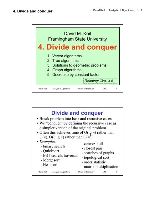
<strong>4.</strong> <strong>Divide</strong> <strong>and</strong> <strong>conquer</strong><br />
David M. Keil<br />
<strong>Framingham</strong> <strong>State</strong> <strong>University</strong><br />
4<strong>4.</strong> <strong>Divide</strong> <strong>and</strong> <strong>conquer</strong><br />
1. Vector algorithms<br />
2. Tree algorithms<br />
3. Solutions to geometric problems<br />
4<strong>4.</strong> Graph algorithms<br />
5. Decrease by constant factor<br />
David Keil Analysis of Algorithms <strong>4.</strong> <strong>Divide</strong> <strong>and</strong> <strong>conquer</strong> 1/12 1<br />
David Keil Analysis of Algorithms 1/12<br />
Reading: Chs. 3-6<br />
<strong>Divide</strong> <strong>and</strong> <strong>conquer</strong><br />
• Break problem into base <strong>and</strong> recursive cases<br />
• We “<strong>conquer</strong>” by defining the recursive case as<br />
a simpler version of the original problem<br />
• Often this achieves time of O(lg n) rather than<br />
O(n), O(n lg n) rather than O(n2 )<br />
• Examples:<br />
- convex hull<br />
- binary search<br />
- closest pair<br />
- Quicksort Q<br />
- BST search, traversal<br />
-Mergesort<br />
- Heapsort<br />
- searches of graphs<br />
- topological sort<br />
- order statistic<br />
- matrix multiplication<br />
David Keil Analysis of Algorithms <strong>4.</strong> <strong>Divide</strong> <strong>and</strong> <strong>conquer</strong> 1/12 2
<strong>4.</strong> <strong>Divide</strong> <strong>and</strong> <strong>conquer</strong><br />
David Keil Analysis of Algorithms 1/12<br />
Topic objectives<br />
4a. Write a recurrence that defines the function<br />
computed by a divide-<strong>and</strong>-<strong>conquer</strong> algorithm<br />
4b. Write <strong>and</strong> solve a time recurrence for a divide-<strong>and</strong><strong>conquer</strong><br />
algorithm<br />
5c. Explain an instance of the divide-<strong>and</strong>-<strong>conquer</strong><br />
approach<br />
5d. Explain <strong>and</strong> use traversal methods for trees<br />
55e. EExplain l i breadth-first b d h fi <strong>and</strong> d depth-first d h fi graph h searches h<br />
5f. Explain the basic binary-search-tree algorithms<br />
5g. Explain the basic algorithms on heaps<br />
David Keil Analysis of Algorithms <strong>4.</strong> <strong>Divide</strong> <strong>and</strong> <strong>conquer</strong> 1/12 3<br />
Inquiry<br />
•Is time scalability a good way to<br />
measure the performance p of computing p g<br />
systems?<br />
• How much does studying design<br />
approaches help us create efficient<br />
solutions?<br />
David Keil Analysis of Algorithms <strong>4.</strong> <strong>Divide</strong> <strong>and</strong> <strong>conquer</strong> 1/12 4
<strong>4.</strong> <strong>Divide</strong> <strong>and</strong> <strong>conquer</strong><br />
1. Vector algorithms<br />
• Binary search<br />
• Quicksort<br />
• Mergesort<br />
• Order statistics<br />
David Keil Analysis of Algorithms <strong>4.</strong> <strong>Divide</strong> <strong>and</strong> <strong>conquer</strong> 1/12 5<br />
Decision trees for search<br />
•The decision tree for a search of<br />
an array must examine each element<br />
• Searching g an unsorted array, y, only y<br />
one element is considered per step<br />
• Hence the tree depth (running time) is O(n)<br />
• Searching a sorted array,<br />
considering the middle element<br />
enables a decision to search only<br />
the right or left half of the array<br />
• Hence the decision tree depth is O(lg n)<br />
David Keil Analysis of Algorithms <strong>4.</strong> <strong>Divide</strong> <strong>and</strong> <strong>conquer</strong> 1/12 6<br />
David Keil Analysis of Algorithms 1/12
<strong>4.</strong> <strong>Divide</strong> <strong>and</strong> <strong>conquer</strong><br />
Binary-search (A, first, last)<br />
if first > last // (i.e., nothing to search)<br />
return false<br />
otherwise<br />
middle ← (first + last) ÷ 2<br />
if A[middle] matches key<br />
return true<br />
otherwise<br />
if A[middle] > key<br />
return Bin-search(A, Bin search(A, first, middle - 1, key)<br />
otherwise<br />
return Bin-search(A, middle + 1, last, key)<br />
> Post: returns true iff key is in A [first…last]<br />
David Keil Analysis of Algorithms <strong>4.</strong> <strong>Divide</strong> <strong>and</strong> <strong>conquer</strong> 1/12 7<br />
Binary search recurrences<br />
Bin-srch(A, x) =<br />
false if |A| = 0<br />
true if A[⎣|A| ÷2⎦] = x<br />
Bi Bin-srch(A[0.. h(A[0 ⎣|A| ÷2⎦]) 2⎦]) if A[⎣|A| ÷2⎦] 2⎦] > x<br />
Bin-srch(A[⎣|A|÷2⎦+1..|A|]) otherwise<br />
Time:<br />
TBin-srch (n) = Θ(1) if n ≤ 1<br />
Θ(1) + 2T 2TBin Bin-srch srch ((n – 1) / 2) otherwise<br />
Recursive call examines at most half the remaining<br />
elements<br />
Solution to recurrence: TBin-srch(n) = Θ(log2n) = Θ(lg n)<br />
David Keil Analysis of Algorithms <strong>4.</strong> <strong>Divide</strong> <strong>and</strong> <strong>conquer</strong> 1/12 8<br />
David Keil Analysis of Algorithms 1/12
<strong>4.</strong> <strong>Divide</strong> <strong>and</strong> <strong>conquer</strong><br />
Solving recurrences:<br />
logarithmic time<br />
T(n) = Θ(1) if n = 1<br />
Θ(1) + T(n / 2) otherwise<br />
Solution: Θ(lg n), because at each of<br />
(n / 2) recursive steps the remaining<br />
time is cut in half<br />
Example: Binary search<br />
David Keil Analysis of Algorithms <strong>4.</strong> <strong>Divide</strong> <strong>and</strong> <strong>conquer</strong> 1/12 9<br />
Logarithms <strong>and</strong> running time<br />
• In algorithm analysis, we can ignore the<br />
base of a logarithm because logbn is<br />
proportional to logcn for all constants b<br />
<strong>and</strong> c<br />
• Θ(lg n) = Θ(log2n) = Θ(logbn) for any base b<br />
• LLogarithmic ith i complexity l it is i desirable d i bl<br />
because the log function grows slowly<br />
David Keil Analysis of Algorithms 1/12<br />
David Keil Analysis of Algorithms <strong>4.</strong> <strong>Divide</strong> <strong>and</strong> <strong>conquer</strong> 1/12 10
<strong>4.</strong> <strong>Divide</strong> <strong>and</strong> <strong>conquer</strong><br />
Correctness of Quicksort<br />
David Keil Analysis of Algorithms 1/12<br />
• To prove: For all i <strong>and</strong> j less than the size of<br />
array A, i < j implies A[i] ≤ A[j]<br />
• Base step: p Property p yto be proven p holds<br />
vacuously for array of size 1, since i = j<br />
• Induction step (summary): This step must show<br />
that if Quicksort leaves each pair of array<br />
elements in correct order for all arrays of size<br />
n, n,t then e the t esa same eis stue true for o all a arrays a ayso of size s e<br />
(n + 1).<br />
• Our argument uses the fact that each partition<br />
is of size n or smaller, so each gets sorted<br />
David Keil Analysis of Algorithms <strong>4.</strong> <strong>Divide</strong> <strong>and</strong> <strong>conquer</strong> 1/12 11<br />
QuickSort(A)<br />
If |A| > 1<br />
(A, pvloc) ← Partition(A)<br />
QuickSort(A[1.. pvloc − 1])<br />
QuickSort(A[pvloc + 1 .. |A|])<br />
Return A<br />
Partition rearranges A such that pvloc is the index of<br />
an element of A, all elements less than A[pvloc] are<br />
to its left, left <strong>and</strong> all elements greater are to its right. right<br />
<strong>Divide</strong>-<strong>and</strong>-<strong>conquer</strong> is used to enable the recursive<br />
calls to sort arrays half as large at each recursive<br />
step<br />
David Keil Analysis of Algorithms <strong>4.</strong> <strong>Divide</strong> <strong>and</strong> <strong>conquer</strong> 1/12 12
<strong>4.</strong> <strong>Divide</strong> <strong>and</strong> <strong>conquer</strong><br />
Partition(A)<br />
pv ← A[1]<br />
j ← 1<br />
k ← 1<br />
for i ← 2to|A| 2 to |A|<br />
if A[ i ] < pv<br />
B[ j ] ← A[ i ]<br />
j ← j + 1<br />
else<br />
C[ k ] ← A[ i ]<br />
k ← k + 1<br />
i ← i + 1<br />
A ← B[1 .. j−1 ] + pv + C[1 .. k−1 ]<br />
return (A, j )<br />
David Keil Analysis of Algorithms 1/12<br />
This algorithm copies<br />
all elements of A less<br />
than pv p into array y B, all<br />
others to array C, <strong>and</strong><br />
copies B, pv, <strong>and</strong> C<br />
back into A. Its running<br />
time is O(n)<br />
David Keil Analysis of Algorithms <strong>4.</strong> <strong>Divide</strong> <strong>and</strong> <strong>conquer</strong> 1/12 13<br />
Partition code<br />
Partitions subarray num[first..last], returns index of pivot value<br />
int partition(int num[], int first, int last)<br />
{<br />
int pivot = num[first];<br />
iint t lleft ft = fi first t + 11, right i ht = llast; t<br />
do {<br />
}<br />
while (left < = right && num[left] < = pivot)<br />
++left;<br />
while (left < = right && num[right] > pivot)<br />
--right;<br />
Repeatedly finds<br />
if (left < right)<br />
leftmost element<br />
swap (num[left], num[right]);<br />
in left partition<br />
} while (left < = right); that should be in<br />
swap (num[first], num[right]); right <strong>and</strong><br />
return right;<br />
rightmost that<br />
Move pivot into middle<br />
should be in left,<br />
David Keil Analysis of Algorithms <strong>4.</strong> <strong>Divide</strong> <strong>and</strong> <strong>conquer</strong> swaps 1/12them 14
<strong>4.</strong> <strong>Divide</strong> <strong>and</strong> <strong>conquer</strong><br />
Quicksort recurrences<br />
Qsort (A) =<br />
A If |A| ≤ 1<br />
Qsort(Left-part Qsort(Left part (A (A, A[1])) + A[1] +<br />
Qsort (Right-part (A, A[1])) otherwise<br />
Left-part (A, x) = sequence of all elts < x<br />
λ if A = λ<br />
A[1]+Left-part(A[2 A[1]+Left part(A[2..|A|],x) |A|] x) if A[1] < x<br />
Left-part(A[2..|A|],x)+A[1] otherwise<br />
Right-part(A, x) mirrors Left-part(A, x)<br />
David Keil Analysis of Algorithms 1/12<br />
David Keil Analysis of Algorithms <strong>4.</strong> <strong>Divide</strong> <strong>and</strong> <strong>conquer</strong> 1/12 15<br />
Complexity of Quicksort (avg. case)<br />
T Quick(n) = 1 if n ≤ 1<br />
O(n) + 2TQuick ( ⎡(n − 1) / 2⎤ )<br />
otherwise<br />
• There are (lg n) levels of recursion because<br />
(n − 1) is repeatedly divided by 2<br />
• There are n steps at each level of recursion to<br />
perform partition<br />
• WWe can toss t out tt term 1 <strong>and</strong> df factor t 2<br />
• Solution: T(n) = O(n lg n)<br />
•This is much better than O(n2 )<br />
David Keil Analysis of Algorithms <strong>4.</strong> <strong>Divide</strong> <strong>and</strong> <strong>conquer</strong> 1/12 16
<strong>4.</strong> <strong>Divide</strong> <strong>and</strong> <strong>conquer</strong><br />
Merge algorithm<br />
A <strong>and</strong> B are sorted arrays; Merge returns a<br />
sorted array containing all elements of A, B<br />
Merge (A, B)<br />
=<br />
A if B = λ<br />
B if A = λ<br />
A[1]+Merge(A[2..|A|], B) if A[1] < B[1]<br />
B[1]+Merge(A, B[2..|B|]) otherwise<br />
Spec: If f A, B are each hsorted d arrays, then h<br />
Merge(A, B) is a sorted array<br />
Problem: Write TMerge(n) recurrence<br />
David Keil Analysis of Algorithms 1/12<br />
David Keil Analysis of Algorithms <strong>4.</strong> <strong>Divide</strong> <strong>and</strong> <strong>conquer</strong> 1/12 17<br />
Mergesort<br />
<strong>Divide</strong>-<strong>and</strong>-<strong>conquer</strong> algorithm: divide array in<br />
two, sort each half, merge the results<br />
Mergesort(A)<br />
If |A| ≤ 1<br />
return A<br />
else<br />
return Merge (Mergesort(A [1 .. |A| / /2]) 2]),<br />
Mergesort(A [|A| / 2 +1.. |A|]))<br />
Problem: Write T Mergesort(n) recurrence<br />
David Keil Analysis of Algorithms <strong>4.</strong> <strong>Divide</strong> <strong>and</strong> <strong>conquer</strong> 1/12 18
<strong>4.</strong> <strong>Divide</strong> <strong>and</strong> <strong>conquer</strong><br />
Order statistics<br />
• Problem: Find kth-highest value in an<br />
unsorted list; e.g., median<br />
• BBrute-force f solution: l i<br />
Kth-highest(A, k) =<br />
A[1] if k = 1 <strong>and</strong> size(A) = 1<br />
min-elt(A) if size(A) = k<br />
Kth-highest(A g ( – min-elt(A), ( ), k – 1) )<br />
otherwise<br />
David Keil Analysis of Algorithms 1/12<br />
David Keil Analysis of Algorithms <strong>4.</strong> <strong>Divide</strong> <strong>and</strong> <strong>conquer</strong> 1/12 19<br />
Computing order statistics<br />
• kth order statistic in a list is the kth element of a<br />
sorted version of the list<br />
• Median edian is sode order statistic s s cw where eekk = ⎡n / 2⎤⎤<br />
• A variable-size-decrease algorithm:<br />
– Choose pivot as in Quicksort<br />
– Partition list, find pivot position p<br />
– If p < ki, find (k – p)th order statistic of right<br />
partition; recurse<br />
– T(n) = T(n / 2) + (n + 1) (average case)<br />
– T(n) ∈θ(n) [error? n vs n+1]<br />
David Keil Analysis of Algorithms <strong>4.</strong> <strong>Divide</strong> <strong>and</strong> <strong>conquer</strong> 1/12 20
<strong>4.</strong> <strong>Divide</strong> <strong>and</strong> <strong>conquer</strong><br />
Order statistic recurrence<br />
OS(k, A) =<br />
A[pivloc(A)] if k = pivloc(A)<br />
OS( OS(pivloc(A) ( ) – k, A[1..pivloc(A)-1] ( )<br />
if k < pivloc(A)<br />
OS(k – pivloc(A), A[pivloc(A)+1, |A|)<br />
otherwise<br />
Pivloc is computed by using the<br />
Partition from Quicksort<br />
David Keil Analysis of Algorithms 1/12<br />
David Keil Analysis of Algorithms <strong>4.</strong> <strong>Divide</strong> <strong>and</strong> <strong>conquer</strong> 1/12 21<br />
2. Tree algorithms<br />
• Tree traversals: Recursively visit<br />
subtrees until subtrees are leaves<br />
• Binary search tree search: Makes<br />
use of BST ordering property <strong>and</strong><br />
average height of binary tree<br />
• Heap algorithms: Make use of<br />
height of complete binary tree<br />
David Keil Analysis of Algorithms <strong>4.</strong> <strong>Divide</strong> <strong>and</strong> <strong>conquer</strong> 1/12 22
<strong>4.</strong> <strong>Divide</strong> <strong>and</strong> <strong>conquer</strong><br />
Inorder traversal<br />
Inorder-traverse (node, op)<br />
1. If node has left child<br />
Inorder-traverse (Left(node), op)<br />
2. Apply operation op to node<br />
3. If node has right child<br />
Inorder-traverse (Right(node), op)<br />
David Keil Analysis of Algorithms 1/12<br />
(Left, parent, right)<br />
• Order for tree above: 1, 3, 5, 6, 7<br />
• Application: Display BST in ascending order<br />
David Keil Analysis of Algorithms <strong>4.</strong> <strong>Divide</strong> <strong>and</strong> <strong>conquer</strong> 1/12 23<br />
Preorder traversal<br />
A node is<br />
operated on as<br />
soon as it is<br />
first visited. visited<br />
Preorder-traverse (node, op)<br />
1. Apply operation op to node<br />
2. If node has left child<br />
Preorder-traverse (Left(node), op)<br />
3. If node has right child<br />
Preorder-traverse (Right(node), op)<br />
• Order for tree above: 3, 1, 6, 5, 7<br />
• Application: Copy tree<br />
David Keil Analysis of Algorithms <strong>4.</strong> <strong>Divide</strong> <strong>and</strong> <strong>conquer</strong> 1/12 24
<strong>4.</strong> <strong>Divide</strong> <strong>and</strong> <strong>conquer</strong><br />
Postorder traversal<br />
A node is<br />
operated on<br />
after its<br />
descendants<br />
Postorder-traverse (node, op)<br />
1. If node has left child<br />
Postorder-traverse (Left(node), op)<br />
2. If node has right child<br />
Postorder-traverse (Right(node), op)<br />
3A 3. Apply l operation ti op tto node d<br />
• Order for tree above: 1, 5, 7, 6, 3<br />
• Application: Deallocate tree<br />
David Keil Analysis of Algorithms 1/12<br />
David Keil Analysis of Algorithms <strong>4.</strong> <strong>Divide</strong> <strong>and</strong> <strong>conquer</strong> 1/12 25<br />
BST search of a subtree<br />
Pointer to subtree root<br />
BST-search (root, key)<br />
If root is null, return false<br />
If root’s data matches key<br />
return true<br />
otherwise<br />
if root’s data > key<br />
return BST-search (left (root), key))<br />
otherwise th i<br />
return BST-search (right (root), key))<br />
Search key<br />
• Initial value of root is root of entire tree<br />
David Keil Analysis of Algorithms <strong>4.</strong> <strong>Divide</strong> <strong>and</strong> <strong>conquer</strong> 1/12 26
<strong>4.</strong> <strong>Divide</strong> <strong>and</strong> <strong>conquer</strong><br />
Complexity of BST-search<br />
TSrch(n) = Θ(1) if n < 2<br />
Θ (1) + T TSSrch(n h(n /2) / 2) otherwise<br />
= Θ(lg n)<br />
David Keil Analysis of Algorithms 1/12<br />
• What are the assumptions of the above?<br />
• Does it apply to best, worst, average cases?<br />
• Compare with binary search<br />
• How does BST-insert compare?<br />
David Keil Analysis of Algorithms <strong>4.</strong> <strong>Divide</strong> <strong>and</strong> <strong>conquer</strong> 1/12 27<br />
A heap is a kind of<br />
complete binary tree<br />
• Solves priority queue problem<br />
• A complete l bi binary tree has h all lll levels l full f llexcept<br />
possibly the bottom one, which is filled from the<br />
left<br />
• Which are complete binary trees?<br />
David Keil Analysis of Algorithms <strong>4.</strong> <strong>Divide</strong> <strong>and</strong> <strong>conquer</strong> 1/12 28
<strong>4.</strong> <strong>Divide</strong> <strong>and</strong> <strong>conquer</strong><br />
David Keil Analysis of Algorithms 1/12<br />
Array implementation of<br />
complete binary tree Java<br />
• Root is A[1] A[0]<br />
• A[i]’s left child is A[ 2i ]; A[2*i + 1]<br />
• Its right child is A[2i + 1] A[2*i + 2]<br />
• Parent of A[ i ] is A[⎣i / 2⎦] A[(i-1)/2]<br />
• If n is size, , height g is ⎡log ⎡ g2n⎤ 2 ⎤<br />
David Keil Analysis of Algorithms <strong>4.</strong> <strong>Divide</strong> <strong>and</strong> <strong>conquer</strong> 1/12 29<br />
Height of a complete binary<br />
tree with n nodes is O(log 2n)<br />
• …because size n approximately<br />
pp y<br />
doubles with each level added<br />
•Or, 2height−1 ≤ n ≤ 2height −1<br />
David Keil Analysis of Algorithms <strong>4.</strong> <strong>Divide</strong> <strong>and</strong> <strong>conquer</strong> 1/12 30
<strong>4.</strong> <strong>Divide</strong> <strong>and</strong> <strong>conquer</strong><br />
A maximum heap<br />
• Heap property: for all i up to array size,<br />
A[i] ≤ A[i / 2]<br />
David Keil Analysis of Algorithms 1/12<br />
David Keil Analysis of Algorithms <strong>4.</strong> <strong>Divide</strong> <strong>and</strong> <strong>conquer</strong> 1/12 31<br />
The Heapify operation<br />
• Heapify(A,i) applies to one node, with<br />
subscript i, of a complete binary tree stored<br />
iin array A<br />
• It assumes that subtrees with roots Leftchild(i)<br />
<strong>and</strong> Right-child(i) already have the<br />
heap property<br />
• Node A[i] may meet or violate heap property<br />
• Heapify(A,i) causes the subtree with root<br />
subscript i to have the heap property<br />
David Keil Analysis of Algorithms <strong>4.</strong> <strong>Divide</strong> <strong>and</strong> <strong>conquer</strong> 1/12 32
<strong>4.</strong> <strong>Divide</strong> <strong>and</strong> <strong>conquer</strong><br />
Intuition for Heapify<br />
David Keil Analysis of Algorithms 1/12<br />
• The algorithm drags the value at a selected<br />
node down to its proper level where heap<br />
propert property applies to it<br />
• It does this by recursively exchanging the<br />
value in the root node with the higherpriority<br />
child of its two children<br />
• CComplexity: l it DDepth th of f complete l t binary bi tree t<br />
with n nodes, i.e., Θ(lg n)<br />
David Keil Analysis of Algorithms <strong>4.</strong> <strong>Divide</strong> <strong>and</strong> <strong>conquer</strong> 1/12 33<br />
Heapify(A,i) for minimum heap<br />
L ← Left( i )<br />
R ← Right( i )<br />
If L = null <strong>and</strong> R = null then return<br />
if L ≤ |A| <strong>and</strong> A[L] <
<strong>4.</strong> <strong>Divide</strong> <strong>and</strong> <strong>conquer</strong><br />
To convert an array to a heap<br />
Overview: Heapify at every non-leaf<br />
node, starting at the bottom<br />
Build-heap(A)<br />
for i ← ⎣|A| / 2⎦ down to 1<br />
Heapify(A,i )<br />
Because leaves don’t<br />
need to be heapified<br />
[SHOW WHY]<br />
Use version for min<br />
or max heap<br />
Analysis: Θ(n lg n)<br />
David Keil Analysis of Algorithms 1/12<br />
David Keil Analysis of Algorithms <strong>4.</strong> <strong>Divide</strong> <strong>and</strong> <strong>conquer</strong> 1/12 35<br />
Extract value from heap<br />
Extract-min (A)<br />
If |A| < 1<br />
throw exception<br />
min ← A[1]<br />
A[1] ← A[|A|]<br />
|A| ← |A| − 1<br />
Heapify(A,1)<br />
Return min<br />
• Returns minimum<br />
value from a min-heap<br />
• Deletes that value<br />
from heap<br />
• Analysis: Θ(lg n)<br />
David Keil Analysis of Algorithms <strong>4.</strong> <strong>Divide</strong> <strong>and</strong> <strong>conquer</strong> 1/12 36
<strong>4.</strong> <strong>Divide</strong> <strong>and</strong> <strong>conquer</strong><br />
Insertion into a min-heap<br />
Heap-insert (A, key)<br />
Heap-size(A) ← Heap-size(A) + 1<br />
i ← Heap-size(A)<br />
while i > 1 <strong>and</strong> A[Parent( i )] > key<br />
A[i ] ← A[Parent( i )]<br />
i ← Parent( i )<br />
A[i ] ← key<br />
David Keil Analysis of Algorithms 1/12<br />
Analysis: Θ(lg n)<br />
because Parent[i] halves i<br />
David Keil Analysis of Algorithms <strong>4.</strong> <strong>Divide</strong> <strong>and</strong> <strong>conquer</strong> 1/12 37<br />
To sort an array using a max-heap<br />
Heapsort(A)<br />
Build-heap(A)<br />
using<br />
for i ← length(A) g ( ) downto 2<br />
exchange A[1] with A[ i ]<br />
Heap-size(A) ← Heap-size(A) − 1<br />
Heapify(A,1)<br />
Analysis: Θ(n lg n)<br />
• In plain language…<br />
Repeatedly extract the highest value<br />
from heap <strong>and</strong> put it at front of a<br />
growing sorted array just after the heap<br />
Replace<br />
extracat<br />
David Keil Analysis of Algorithms <strong>4.</strong> <strong>Divide</strong> <strong>and</strong> <strong>conquer</strong> 1/12 38
<strong>4.</strong> <strong>Divide</strong> <strong>and</strong> <strong>conquer</strong><br />
Terminology about heaps<br />
Johnsonbaugh- Cormen-Leiserson-<br />
Schaefer Rivest<br />
Sift-down Heapify<br />
Heapify Build-heap<br />
Largest-delete Extract-max<br />
• Our reference is Cormen-Leiserson-Rivest<br />
• Lesson: In computer science, law of frontier<br />
operates for terminology<br />
David Keil Analysis of Algorithms 1/12<br />
David Keil Analysis of Algorithms <strong>4.</strong> <strong>Divide</strong> <strong>and</strong> <strong>conquer</strong> 1/12 39<br />
3. Solutions to<br />
geometric problems<br />
Convex hull problem<br />
• The Convex hull of a set of points is a subset of<br />
ordered pairs (on a Cartesian plane) that define a<br />
polygon with no concave series of edges<br />
(“dents”); i.e., the posts of the shortest fence that<br />
would enclose all the points<br />
• I.e., find smallest convex polygon that contains<br />
all of a set of points<br />
David Keil Analysis of Algorithms <strong>4.</strong> <strong>Divide</strong> <strong>and</strong> <strong>conquer</strong> 1/12 40
<strong>4.</strong> <strong>Divide</strong> <strong>and</strong> <strong>conquer</strong><br />
Convex hull<br />
divide-<strong>and</strong>-<strong>conquer</strong> solution<br />
• Find leftmost <strong>and</strong> rightmost points in set, P 1 <strong>and</strong><br />
P 2 (these are in the convex hull)<br />
2 ( )<br />
• Define upper <strong>and</strong> lower areas as separated by the<br />
line segment (P 1, P 2)<br />
• In each area, find farthest point from segment,<br />
recursively find triangles defined by farthest<br />
points -- EXPLAIN<br />
• Combine upper <strong>and</strong> lower hulls<br />
• Average case: T(n) = θ(n lg n), worst: θ(n2 )<br />
David Keil Analysis of Algorithms 1/12<br />
diagram<br />
David Keil Analysis of Algorithms <strong>4.</strong> <strong>Divide</strong> <strong>and</strong> <strong>conquer</strong> 1/12 41<br />
Closest pair (of a set of points)<br />
• Given a set of ordered pairs (points on a Cartesian<br />
plane) find the two points that are closest together.<br />
• Algorithm: g<br />
1. <strong>Divide</strong> set into two vertical areas<br />
2. Find closest pair in each<br />
3. Choose closest of these two<br />
<strong>4.</strong> See if any pairs crossing boundary are closer<br />
• T(n) = 2T(n / 2) + M(n), where M(n) is time to<br />
merge the solutions to subproblems<br />
• T(n) ∈θ(n lg n)<br />
• Brute force approach yields θ(n2 )<br />
David Keil Analysis of Algorithms <strong>4.</strong> <strong>Divide</strong> <strong>and</strong> <strong>conquer</strong> 1/12 42
<strong>4.</strong> <strong>Divide</strong> <strong>and</strong> <strong>conquer</strong><br />
<strong>4.</strong> Graph algorithms<br />
• Depth-first search: Label each vertex of<br />
graph with a number in order visited, using<br />
the strategy of exhausting one path before<br />
backtracking to start at a new edge<br />
• Breadth-first search: Label each vertex,<br />
using the strategy of visiting each vertex<br />
adjacent to the current one at each stage<br />
• Topological sort of a dag (2 versions): see<br />
below<br />
David Keil Analysis of Algorithms 1/12<br />
David Keil Analysis of Algorithms <strong>4.</strong> <strong>Divide</strong> <strong>and</strong> <strong>conquer</strong> 1/12 43<br />
Depth-first search of graph<br />
GDFS(G) G = (V, E)<br />
> Pre: there is a vertex v in V s.t. Mark[v] = 0<br />
count ← 0<br />
for each vertex v ∈ V do<br />
if Mark(v) = 0<br />
vdfs(v, count)<br />
return Mark<br />
> Post: Vertices are marked in order of<br />
> some DFS traversal<br />
Running time: Θ(n)<br />
David Keil Analysis of Algorithms <strong>4.</strong> <strong>Divide</strong> <strong>and</strong> <strong>conquer</strong> 1/12 44
<strong>4.</strong> <strong>Divide</strong> <strong>and</strong> <strong>conquer</strong><br />
David Keil Analysis of Algorithms 1/12<br />
Depth-first search from vertex<br />
vdfs(v, V ) // recursive<br />
count ← count + 1<br />
Mark[v] ← count<br />
For each vertex w ∈ V adjacent to v do<br />
if Mark[w] = 0<br />
vdfs(w, V)<br />
> Post: v’s mark is set<br />
Challenge: show termination<br />
[See URL found by B. Grozier]<br />
David Keil Analysis of Algorithms <strong>4.</strong> <strong>Divide</strong> <strong>and</strong> <strong>conquer</strong> 1/12 45<br />
Breadth-first search<br />
• Checks all vertices 1 edge from origin, then<br />
2 edges, then 3, etc., to find path to<br />
destination<br />
• If G = 〈{a..i}, (a,b), (a,c), (a,d), (c,d), (b,e),<br />
(b, f ), (c, g), (g, h), (g, i), (h, i) 〉, <strong>and</strong><br />
– BFS input is G, a, f, then<br />
– Order Odeof o search seac is s(a,b), (a,b), (a,c), (a,d), (b,e),<br />
(b, f )<br />
[pic]<br />
David Keil Analysis of Algorithms <strong>4.</strong> <strong>Divide</strong> <strong>and</strong> <strong>conquer</strong> 1/12 46
<strong>4.</strong> <strong>Divide</strong> <strong>and</strong> <strong>conquer</strong><br />
Breadth-first search<br />
BFS(G)<br />
count ← 0<br />
G = (V, E) Iterative<br />
for each vertex v ∈ V do<br />
if Mark(v) = 0 • Proceeds concentrically<br />
bfs(v)<br />
bfs(v)<br />
count ← count + 1<br />
Mark (v) ← count<br />
Queue ← ( v )<br />
While not empty(queue) do<br />
David Keil Analysis of Algorithms 1/12<br />
• UUses queue rather h than h<br />
DFS’s stack<br />
• See example (pic)<br />
For each vertex w ∈ V adjacent to front(queue) do<br />
if Mark(w) = 0<br />
count ← count + 1<br />
append w to queue<br />
Remove front of queue<br />
David Keil Analysis of Algorithms <strong>4.</strong> <strong>Divide</strong> <strong>and</strong> <strong>conquer</strong> 1/12 47<br />
Topological sort of dag<br />
• dag: directed acyclic graph<br />
• Example: a listing of courses in a prerequisite<br />
relation so that no course is taken before its<br />
prereqs<br />
• Algorithm 1: Perform DFS, arrange vertices<br />
in reverse order of becoming dead-ends<br />
• Algorithm 2: Find source (vertex lacking inedges),<br />
delete it <strong>and</strong> its adjacent vertices<br />
recursively. Order of deletion is topological<br />
ordering<br />
David Keil Analysis of Algorithms <strong>4.</strong> <strong>Divide</strong> <strong>and</strong> <strong>conquer</strong> 1/12 48
<strong>4.</strong> <strong>Divide</strong> <strong>and</strong> <strong>conquer</strong><br />
5. Decrease by constant factor<br />
• Looking for solutions where<br />
T(n) = T(n / b) + f (n)<br />
• If T( T(n) ) = T( T(n/2) /2) + f ( (n), )th then depth d thof frecursion i<br />
is log2n • Examples:<br />
– Binary search, where f(n) = 1,<br />
hence solution is O(lg (g n) )<br />
– Quicksort, where f (n) = n,<br />
hence solution is O(n lg n)<br />
David Keil Analysis of Algorithms 1/12<br />
David Keil Analysis of Algorithms <strong>4.</strong> <strong>Divide</strong> <strong>and</strong> <strong>conquer</strong> 1/12 49<br />
Master Theorem (“Main<br />
Recurrence Theorem”)<br />
•Let T(n) = aT(⎣n/b⎦) + f (n)<br />
• Let f (n) ∈ θ(nd Let f (n) ∈ θ(n ), d ≥ 0<br />
• Then T(n) ∈<br />
– θ(nd ), if a < bd – θ(nd lg n), if a = bd – θ(n logba), if a > bd • This theorem simplifies solving some<br />
recurrence equations for divide-<strong>and</strong>-<strong>conquer</strong><br />
algorithms<br />
• Example: Binary search<br />
David Keil Analysis of Algorithms <strong>4.</strong> <strong>Divide</strong> <strong>and</strong> <strong>conquer</strong> 1/12 50
<strong>4.</strong> <strong>Divide</strong> <strong>and</strong> <strong>conquer</strong><br />
Applying the Master Theorem<br />
• Let T(n) = aT(n/b) + f (n), f (n) ∈θ(nd )<br />
• Then by Master Thm., T(n) ∈θ(nd lg n), if a = bd • EExamples: l<br />
– (Binary search) T(n) = T(n/2) + O(1),<br />
so a = 1, b = 2, d = 0, hence a = bd , f(n) = 1,<br />
hence T(n) ∈θ(lg n)<br />
– (Quicksort) T(n) = 2T(n/2) + O(n),<br />
so a = 2, b = 2, d = 1, hence a = bd , , ,<br />
• Master Theorem does not apply to linear search,<br />
quadratic sorts, or exponential-time algorithms<br />
David Keil Analysis of Algorithms 1/12<br />
David Keil Analysis of Algorithms <strong>4.</strong> <strong>Divide</strong> <strong>and</strong> <strong>conquer</strong> 1/12 51<br />
Servant Conjecture (Keil)<br />
•Let T(n) = T(n − k) + f (n), with k constant,<br />
f (n) ∈θ(n d )<br />
• Th Then T( T(n) ) ∈ θ( θ(n f ( (n)) ))<br />
•Examples:<br />
– Linear search is θ(n)<br />
– Bubble, Selection, Insertion sorts are<br />
θ(n2 θ(n ) 2 )<br />
• The Servant Conjecture is useful, <strong>and</strong> is<br />
probably easily proven – try it!<br />
David Keil Analysis of Algorithms <strong>4.</strong> <strong>Divide</strong> <strong>and</strong> <strong>conquer</strong> 1/12 52
<strong>4.</strong> <strong>Divide</strong> <strong>and</strong> <strong>conquer</strong><br />
binary search<br />
binary-tree traversal<br />
breadth-first search<br />
BST search<br />
dag<br />
decrease by constant<br />
factor<br />
depth-first search<br />
di directed d acyclic li graphh<br />
divide <strong>and</strong> <strong>conquer</strong><br />
Concepts<br />
David Keil Analysis of Algorithms 1/12<br />
extract-min<br />
heap<br />
heapify pfy<br />
heapsort<br />
inorder traversal<br />
logarithmic time O(lg n)<br />
Master Theorem<br />
mergesort<br />
order d statistic i i<br />
Quicksort<br />
topological sort<br />
tree traversal<br />
David Keil Analysis of Algorithms <strong>4.</strong> <strong>Divide</strong> <strong>and</strong> <strong>conquer</strong> 1/12 53<br />
References<br />
Cormen, Leiserson, Rivest. Algorithms. MIT<br />
Press, 1997.<br />
A. Levitin. The Design <strong>and</strong> Analysis of<br />
Algorithms. Addison Wesley, 2003.<br />
Chapters 4-5.<br />
R. Johnsonbaugh <strong>and</strong> M. Schaefer.<br />
Al Algorithms. ith PPearson PPrentice ti Hall, H ll 200<strong>4.</strong> 2004<br />
Chs. 3-6.<br />
Notation ideas by A. Bilodeau, 2006.<br />
David Keil Analysis of Algorithms <strong>4.</strong> <strong>Divide</strong> <strong>and</strong> <strong>conquer</strong> 1/12 54