Economic Reliability Acceptance Sampling Plan for Generalized ...

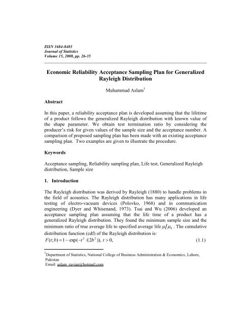
ISSN 1684-8403
Journal of Statistics
Volume 15, 2008, pp. 26-35
________________________________________________________________________
Economic Reliability Acceptance Sampling Plan for Generalized
Rayleigh Distribution
Abstract
Muhammad Aslam 1
In this paper, a reliability acceptance plan is developed assuming that the lifetime
of a product follows the generalized Rayleigh distribution with known value of
the shape parameter. We obtain test termination ratio by considering the
producer’s risk for given values of the sample size and the acceptance number. A
comparison of proposed sampling plan has been made with an existing acceptance
sampling plan. Two examples are given to illustrate the procedure.
Keywords
Acceptance sampling, Reliability sampling plan, Life test, Generalized Rayleigh
distribution, Sample size
1. Introduction
The Rayleigh distribution was derived by Rayleigh (1880) to handle problems in
the field of acoustics. The Rayleigh distribution has many applications in life
testing of electro-vacuum devices (Polovko, 1968) and in communication
engineering (Dyer and Whisenand, 1973). Tsai and Wu (2006) developed an
acceptance sampling plan assuming that the life time of a product has a
generalized Rayleigh distribution. They found the minimum sample size and the
minimum ratio of true average life to specified average life 0
. The cumulative
distribution function (cdf) of the Rayleigh distribution is:
2 2
F ( t;
b)
1
exp( t
/(2b
)), t 0,
(1.1)
1 Department of Statistics, National College of Business Administration & Economics, Lahore,
Pakistan
Email: aslam_ravian@hotmail.com

Economic Reliability Acceptance Sampling Plan for Generalized Rayleigh Distribution
_______________________________________________________________________________
where b>0 is the scale parameter. The failure rate is an increasing linear function
of time, which makes it suitable for modeling the lifetime of electronic
components. Voda (1976) derived a generalized version of the Rayleigh
distribution called the generalized Rayleigh distribution (GRD), whose cdf is
given by:
2
k 2 j t
/
( t / )
e
Fk
( t;
) 1
,
(1.2)
j0
j!
where k is a positive integer called the shape parameter and λ>0 is the scale
2
parameter. When k=0 and 2b , the cdf given in (1.2) reduces to (1.1). The ith
moment of the random variable T having GRD is:
1/2
i
ki/ 2 1
i/2
[ ]
, i 1,2,....
1/2
E T
k 1
So the mean of GRD is given by:
27
(1.3)
1/2
E[ T]
m
(1.4)
where m k 3/ 2 k
1
.
The quality of the product is tested on the basis of few items taken from an
infinite lot. The statistical test can be stated as: Let be the true average life and
0
be the specified average life of a product. Based on the failure data, we want
to test the hypotheses H : against H :
0 0
1 0
. A lot is considered as good
if 0
and bad if 0
. This hypothesis is tested using the acceptance
sampling scheme as: In a life test experiment, a sample of size n selected from a
lot of products is put on the test. The experiment is terminated at a pre-assigned
timet 0
. When we set acceptance number as c , H
0
is rejected if more than c
failures are recorded before timet 0
. If there are c or fewer failures before t 0
, then
H
0
is accepted. Producer’s risk and the consumer’s risk are associated with
acceptance sampling. The probability of rejecting a good lot is called the
producer’s risk say and the probability of accepting a bad lot is known as
consumer’s risk, say . A well acceptance sampling plan minimizes both the
risks.

28
Aslam
_______________________________________________________________________________
Truncated life tests of this type have been developed by Sobel and Tischendrof
(1959), Goode and Kao (1961) for Weibull distribution, Kantam and Rosaiah
(1998) for half logistic distribution, Kantam et al. (2001) for log-logistic
distribution, Baklizi (2003) for the Pareto distribution of the second kind, Rosaiah
and Kantam (2005) for inverse Rayleigh distribution, Rosaiah et al. (2006) for
exponentiated log-logistic distribution, Rosaiah et al. (2007) developed the
reliability plans for exponentiated log-logistic distribution, Aslam (2007) for the
Rayleigh distribution, Balakrishnan et al. (2007) for the generalized Birnbaum-
Saunders distribution, Aslam and Shahbaz (2007) for the generalized exponential
distribution, Rosaiah et al. (2008) for the inverse Rayleigh, and Aslam and
Kantam (2008) for the Birnbaum-Saunders distribution. We propose a reliability
acceptance sampling plan when the lifetime of a product follows the generalized
Rayleigh distribution. Further, it is assumed that the shape parameter of this
distribution is known. The rest of the paper is organized as: design of the
proposed plan is given in Section 2, the comparative study with existing plan is
given in Section 3. Some Tables are given at the end of the paper.
2. Design of Proposed Plan
We are interested in designing a sampling plan which ensures that the true
average life is greater than the specified average life. We propose the following
acceptance sampling plan based on truncated life test:
i. Select n d r ( r c 1, d 2,3, ) items and put them on test.
ii. Select the acceptance number c and termination timet 0
.
iii. Terminate the experiment if more than c failures are recorded before
termination time and reject the lot. Accept the lot if c or fewer failures
occur before termination time.
Suppose that the lifetime of a product follows the GRD with cdf given in (1.2). It
would be convenient to determine the termination time t0
as a multiple of the
specified average life 0
. We assume that the lot size is large enough so that the
binomial theory can be applied. Thus the acceptance or rejection criterion of the
lot is equivalent to the acceptance or rejection of the hypothesis that 0
. For
more justification about the use of the binomial distribution in proposed plan, one

Economic Reliability Acceptance Sampling Plan for Generalized Rayleigh Distribution
_______________________________________________________________________________
may refer to Stephens (2001). The lot acceptance probability is given as:
c
n
i ni
L(
p)
p
(1 p)
,
(2.1)
i0
i
where p is the probability that an item fails before termination time and is given
by:
2
2 j am
am
0
e
k
0
p 1
.
(2.2)
j0
j!
for k =0, 1 and 2 m is 0.886227, 1.32934 and 1.66168, respectively.
29
Now, we find the minimum termination ratio for some specified producer’s risk,
sample size n r d and the acceptance number d
c 1
when the following
inequality is satisfied:
n
ir
n
i
ni
p0 ( 1 p0
) 1
.
i
(2.3)
Tables 1-3 represent the termination time according to various values of shape
parameter, acceptance number, sample size and two values of producer’s risk. It is
clear from the Table 1 as the sample size increases for fixed value of r , the
termination ratios decrease. If shape values increase, the termination ratio also
increases. For example, when r 4, n 40 , k 0 and =0.05, the termination
ratio is 0.213. Keeping the other quantities same and k 1, the termination ratio
is 0.405.
3. Comparative Study
The upper entry in each cell of Table 4 corresponds to the proportion of t 0
a
of the proposed test plan with k 0 . The lower entry corresponds to the similar
quantity of the sampling plan of Tsai and Wu (2006). These entries reveal that the
termination ratio of the proposed test plans is smaller than they are for the plans in
Tsai and Wu (2006).

30
Aslam
_______________________________________________________________________________
Example 1
Suppose that the life time of a product follows the GRD with k 0 . An
experimenter wants to run an experiment at t =1500 hours ensuring that the
specified average life is at least 1000 hours. This leads to the termination ratio
1.5. Let the producer’s risk be 0.05. The corresponding values of n and c from
Table 1 of Tsai and Wu (2006) are 4 and 1, respectively. The sampling plan
( n 4, c 1, t 0
1.500) is stated as: if during 1500 hours no more than 1 failure
out of 4 is recorded, the lot is accepted, otherwise rejected. For the same sampling
plan the termination ratio from Table 1 is 0.362. Thus, the proposed plan will be
( n 4, c 1, t0 0
0.362) which is implemented as: We reject the product if
more than 1 failure is observed during the 362 hours, otherwise we accept it.
In both approaches the acceptance number, the sample size, the producer’s risk
and the final decision about the lot are the same. But the decision on the first
approach equates to 1500 st hours and in the second approach, it equates to 362 st
hours. Hence, the proposed approach is preferable to that of the first approach.
Example 2
Consider a problem associated with reliability provided by Wood (1996) and
analyzed from the acceptance sampling viewpoint by Rosaiah and Kantam
(2005), Rosaiah at al. (2007) and Balakrishnan et al. (2007). The ordered failure
times of the release of software given in terms of hours from the starting of the
execution of the software are regarded as ordered sample of size 14 with the
x i . The ordered data are 519, 968, 1430, 1893,
failure times as , ( 1,2,..,14)
i
2490, 3058, 3625, 4422, 5218, 5823, 6539, 7083, 7487, and 7846.
First we check whether the GRD can be used or not for the above data. The MLE
of ˆ is 13321429. The Kolmogorov-Smirnov distance between the observed and
fitted distribution is 0.2447 which is less than the Kolmogorov-Smirnov Table
value of 0.314. Hence, it is reasonable to assume that lifetime of this product
follows GRD with k=0.
Case I:
Suppose that the specified average life of software product is 1000 hours. Let the
producer’s risk be 0.01. The termination time to test the product from Table 1 of
Tsai and Wu (2006) is 800 hours with corresponding c 1. Then the acceptance
plan is ( n 14, c 1, t 0
.8) . According to existing plan the product is rejected

Economic Reliability Acceptance Sampling Plan for Generalized Rayleigh Distribution
_______________________________________________________________________________
if more than 1 failure is observed during 800 hours. The experiment is
terminated if 2 failures occur before 800 hours; or end time of the experiment,
whichever occurs earlier. From the data we see that only one failure occurs
before 800 hours, therefore we accept this product with 99% confidence.
Case II:
From Table 1, the value of termination ratio is 0.115 for the same software data
as in Example 2. Since the acceptable average life is to be 1000 hours, we get
t0 0.1151000 115 hours (approximately). The proposed sampling plan is
( n 14, c 1, t0 0
.115) . We put 14 items on test. The lot of product will be
accepted if no more than 1 failure occurs before 115 hours. In this approach we
see that among 14 failures, there is no failure before 115 hours, therefore we
accept the product.
Acknowledgements
The author would like to thank the reviewers and Editors for several valuable
comments.
References
1. Aslam, M. (2007). Double acceptance sampling based on truncated life tests
in Rayleigh distribution. European Journal of Scientific Research, 17(4),
605-611.
2. Aslam, M. and Kantam, R. R. L. (2008). Economic acceptance sampling
based on truncated life tests in the Birnbaum-Saunders distribution. Pakistan
Journal of Statistics, 24(4), 269-276.
3. Aslam, M. and Shahbaz, M. Q. (2007). Economic reliability tests plans using
the generalized exponential distribution, Journal of Statistics, 14, 52-59.
4. Baklizi, A. (2003) Acceptance sampling based on truncated life tests in the
Pareto distribution of the second kind. Advances and Applications in
Statistics, 3 (1), 33-48.
5. Balakrishnan, N., Leiva, V. and Lopez, J. (2007). Acceptance sampling plans
from truncated life tests based on the generalized Birnbaum-Saunders
distribution. Communication in Statistics-Simulation and Computation, 36,
643-656.
6. Dyer, D. D. and Whisenand, C. W. (1973). Best linear unbiased estimator of
the parameter of the Rayleigh distribution-Part I: Small sample theory for
censored order statistics, IEEE Transaction on Reliability, 22, 27-34.
31

32
Aslam
_______________________________________________________________________________
7. Goode, H. P. and Kao, J. H. K (1961). Sampling plans based on the Weibull
distribution, Proceedings of the Seventh National Symposium on Reliability
and Quality Control, Philadelphia, Pennsylvania, 24-40.
8. Kantam, R.R. L. and Rosaiah, K. (1998). Half logistic distribution in
acceptance sampling based on life tests, IAPQR Transactions, 23(2), 117-125.
9. Kantam, R.R.L., Rosaiah, K. and Srinivasa Rao,G. (2001). Acceptance
sampling based on life test: log-logistic model, Journal of Applied Statisics,
28(1), 121-128.
10. Polovko, A. M. (1968). Fundamentals of Reliability Theory. Academic Press,
New York.
11. Rayleigh, J. W. S. (1880). On the resultant of a large number of vibrations of
the same pitch and of arbitrary phase, Philosophical Magazine, 5 th series, 10,
73-78.
12. Rosaiah, K. and Kantam, R.R.L. (2005). Acceptance Sampling Based on the
Inverse Rayleigh Distribution, Economic Quality Control, 20(2), 277—286.
13. Rosaiah, K., Kantam, R. R. L. and Reddy, J. R. (2008). Economic reliability
test plan with inverse Rayleigh variate, Pakistan Journal of Statistics, 24, 57-
65.
14. Rosaiah, K., Kantam, R.R.L. and Santosh Kumar, Ch. (2006) Reliability of
test plans for exponentiated log-logistic distribution, Economic Quality
Control, 21(2), 165-175.
15. Rosaiah, K., Kantam, R.R.L. and Santosh Kumar, Ch. (2007). Exponentiated
log-logistic distribution- An economic reliability test plan, Pakistan Journal of
Statistics, 23(2), 165-175.
16. Sobel, M. and Tischendrof, J. A. (1959). Acceptance sampling with new life
test objectives, Proceedings of Fifth National Symposium on Reliability and
Quality Control, Philadelphia, Pennsylvania, 108-118.
17. Stephens, K. S. (2001). The Handbook of Applied Acceptance Sampling:
Plans, Procedures and Principles, ASQ Quality Press, Milwaukee, WI.
18. Tsai, Tzong-Ru and Wu, Shuo-Jye (2006). Acceptance sampling based on
truncated life tests for generalized Rayleigh distribution, Journal of Applied
Statistics, 33(6), 595-600.
19. Voda, V. Gh. (1976). Inferential procedures on a generalized Rayleigh variate,
I, Aplikace Mathematiky, 21, 395-412.
20. Wood, A. (1996). Predicting software reliability, IEEE Transactions on
Software Engineering, 22, 69-77.

Economic Reliability Acceptance Sampling Plan for Generalized Rayleigh Distribution 33
_______________________________________________________________________________
Table 1: Test termination ratios under GRD with k 0
r n 2r
3r 4r 5r 6r 7r 8r 9r 10r
0.05
1 0.181 0.147 0.127 0.114 0.104 0.097 0.090 0.085 0.081
2 0.362 0.287 0.246 0.218 0.197 0.183 0.171 0.160 0.152
3 0.459 0.362 0.308 0.272 0.248 0.228 0.212 0.197 0.189
4 0.522 0.407 0.346 0.307 0.278 0.256 0.239 0.225 0.213
5 0.566 0.441 0.374 0.331 0.299 0.276 0.257 0.234 0.228
6 0.599 0.465 0.394 0.348 0.315 0.290 0.269 0.254 0.240
7 0.624 0.484 0.409 0.361 0.328 0.302 0.281 0.264 0.249
8 0.645 0.499 0.422 0.373 0.346 0.311 0.289 0.272 0.257
0.01
1 0.079 0.064 0.055 0.051 0.046 0.043 0.039 0.038 0.036
2 0.233 0.186 0.159 0.141 0.126 0.115 0.108 0.102 0.097
3 0.335 0.264 0.225 0.197 0.181 0.166 0.155 0.146 0.137
4 0.402 0.317 0.269 0.238 0.216 0.197 0.185 0.174 0.165
5 0.455 0.355 0.301 0.266 0.241 0.222 0.207 0.195 0.184
6 0.490 0.383 0.326 0.288 0.261 0.234 0.224 0.210 0.199
7 0.522 0.407 0.344 0.305 0.276 0.254 0.237 0.222 0.211
8 0.549 0.424 0.360 0.319 0.289 0.266 0.245 0.232 0.219
Table 2: Test termination ratios under GRD with k 1
r n 2r
3r 4r 5r 6r 7r 8r 9r 10r
0.05
1 0.371 0.333 0.309 0.291 0.278 0.267 0.257 0.250 0.243
2 0.544 0.478 0.439 0.411 0.390 0.374 0.360 0.349 0.339
3 0.626 0.544 0.497 0.465 0.440 0.421 0.405 0.392 0.381
4 0.674 0.584 0.532 0.496 0.470 0.449 0.432 0.417 0.405
5 0.708 0.610 0.555 0.517 0.489 0.467 0.449 0.434 0.421
6 0.732 0.630 0.572 0.533 0.504 0.481 0.462 0.447 0.433
7 0.751 0.645 0.585 0.545 0.515 0.491 0.472 0.456 0.443
8 0.766 0.657 0.595 0.554 0.523 0.500 0.480 0.464 0.450

34
Aslam
_______________________________________________________________________________
Continued
r n 2r
3r 4r 5r 6r 7r 8r 9r 10r
0.01
1 0.242 0.218 0.202 0.191 0.182 0.175 0.170 0.164 0.160
2 0.427 0.376 0.347 0.326 0.309 0.297 0.286 0.277 0.267
3 0.522 0.456 0.418 0.391 0.371 0.355 0.342 0.331 0.322
4 0.581 0.505 0.461 0.431 0.408 0.391 0.376 0.364 0.353
5 0.622 0.539 0.491 0.458 0.434 0.415 0.399 0.386 0.375
6 0.653 0.564 0.513 0.479 0.453 0.433 0.416 0.403 0.391
7 0.677 0.583 0.530 0.494 0.468 0.447 0.430 0.415 0.403
8 0.696 0.599 0.544 0.507 0.479 0.458 0.440 0.425 0.413
Table 3: Test termination ratios under GRD with k 2
r n 2r
3r 4r 5r 6r 7r 8r 9r 10r
0.05
1 0.474 0.439 0.415 0.398 0.385 0.374 0.365 0.358 0.351
2 0.628 0.570 0.535 0.511 0.492 0.477 0.464 0.453 0.444
3 0.697 0.628 0.587 0.558 0.537 0.520 0.505 0.493 0.483
4 0.738 0.662 0.617 0.586 0.563 0.544 0.529 0.516 0.505
5 0.766 0.684 0.637 0.605 0.580 0.561 0.545 0.532 0.520
6 0.786 0.701 0.652 0.618 0.593 0.573 0.556 0.543 0.531
7 0.802 0.713 0.663 0.628 0.602 0.582 0.565 0.551 0.539
8 0.815 0.723 0.672 0.636 0.610 0.589 0.572 0.558 0.545
0.01
1 0.350 0.325 0.309 0.297 0.287 0.280 0.273 0.268 0.263
2 0.525 0.479 0.451 0.432 0.416 0.404 0.394 0.385 0.376
3 0.609 0.551 0.517 0.493 0.474 0.460 0.447 0.437 0.428
4 0.660 0.594 0.556 0.529 0.508 0.492 0.479 0.468 0.458
5 0.694 0.623 0.582 0.553 0.531 0.514 0.500 0.488 0.478
6 0.720 0.645 0.601 0.571 0.548 0.530 0.515 0.503 0.492
7 0.740 0.661 0.616 0.585 0.561 0.543 0.527 0.514 0.503
8 0.756 0.674 0.628 0.595 0.571 0.552 0.537 0.524 0.512

Economic Reliability Acceptance Sampling Plan for Generalized Rayleigh Distribution 35
_______________________________________________________________________________
Table 4: Comparison of test termination ratio for k=0
r n 2r
3r 4r 5r 6r 7r 8r 9r 10r
0.05
1 0.104
0.800
2 0.160
0.600
3 0.212
0.600
4 0.407
1.000
5 0.276
0.600
6
7
8
0.01
1 0.079
2.000
2 0.115
0.800
3
4 0.402
1.500
5
6
7
8